THE EXCEL 2013 SCREENMany items you see on the Excel screen are standard in most other Microsoft software programs like Word, PowerPoint and previous versions of Excel. Some elements are specific to Excel.

WORKBOOKAlso called a spreadsheet, the Workbook is a unique file created by Excel.

TITLE BAR

The Title bar displays both the name of the application and the name of the spreadsheet.

THE RIBBON

The Ribbon replaces the menu bars and toolbars found in earlier versions of Office products. The Ribbon contains all of the commands you'll need in order to do common tasks. It contains multiple tabs, each with several groups of commands, and you can add your own tabs that contain your favorite commands. Some groups have an arrow in the bottom-right corner that you can click to see even more commands.

COLUMN HEADINGS

Each Excel spreadsheet contains 256 columns. Each column is named by a letter or combination of letters.

ROW HEADINGSEach spreadsheet contains 65,536 rows. Each row is named by a number.

NAME BOX

Shows the address of the current selection or active cell.

FORMULA BAR

Displays information entered-or being entered as you type-in the current or active cell. The contents of a cell can also be edited in the Formula bar.

CELL

A cell is an intersection of a column and row. Each cell has a unique cell address. In the picture above, the cell address of the selected cell is B3. The heavy border around the selected cell is called the cell pointer.

THE CELLAn Excel worksheet is made up of columns and rows. Where these columns and rows intersect, they form little boxes called cells. The active cell, or the cell that can be acted upon, reveals a dark border. All other cells reveal a light gray border. Each cell has a name. Its name is comprised of two parts: the column letter and the row number.

Row Heading Cell Address Cell Pointer

Column Heading

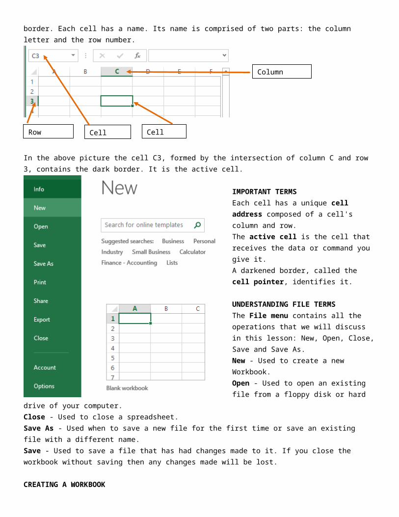
In the above picture the cell C3, formed by the intersection of column C and row 3, contains the dark border. It is the active cell.

IMPORTANT TERMSEach cell has a unique cell address composed of a cell's column and row.The active cell is the cell that receives the data or command you give it.A darkened border, called the cell pointer, identifies it.

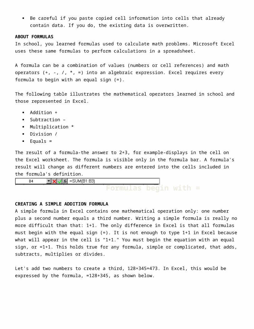
UNDERSTANDING FILE TERMSThe File menu contains all the operations that we will discuss in this lesson: New, Open, Close, Save and Save As.New - Used to create a new Workbook.Open - Used to open an existing file from a floppy disk or hard drive of your computer.Close - Used to close a spreadsheet.Save As - Used when to save a new file for the first time or save an existing file with a different name.Save - Used to save a file that has had changes made to it. If you close the workbook without saving then any changes made will be lost.

CREATING A WORKBOOKA blank workbook is displayed when Microsoft Excel XP is first opened. You can type information or design a layout directly in this blank workbook.

Choose File New from the menu bar.

The New Workbook task pane opens and Blank Workbook is your first option displayed. Double Click “Blank Workbook” and a new workbook opens on your screen.

OPENING A WORKBOOKYou can open any workbook that has previously been saved and given a name.

To Open an Existing Excel Workbook:

Choose File Open from the menu bar.The Open dialog box opens.Click the drive, folder, or Internet location that contains the file you want to open.

In the folder list, open the folder that contains the file. Once the file is displayed, click on the file you want to open.

Click the Open button.

ENTERING TEXT IN A CELL

You can enter three types of data in a cell: text, numbers, and formulas. Text is any entry that is not a number or formula. Numbers are values used when making calculations. Formulas are mathematical calculations.To Enter Data into a Cell:

Click the cell where you want to type information. Type the data. An insertion point appears in the cell as the data is typed.

The data can be typed in either the cell or the Formula bar. Data being typed appears in the both active cell and in the formula bar.

Notice the Cancel and Enter buttons in the formula bar.

Click the Enter button to end the entry and turn off the formula bar buttons. (or hit enter) Note - Excel's AutoComplete feature keeps track of previously-entered text. If the first few characters you type

in a cell match an existing entry in that column, Microsoft Excel fills in the remaining characters for you. To get rid of data that you have in a cell and no longer want, click in the cell and backspace or delete it out in the

formula bar.

PERFORMING UNDO AND REDOSometimes, you might do something to a spreadsheet that you didn't mean to do, like type the wrong number in a cell. Excel allows you to undo an operation. Use the Undo button on the Standard toolbar to recover an error. The last single action is recoverable.

To Undo Recent Actions (typing, formatting, etc), One at a Time:

Click the Undo button.

To Undo Several Recent Actions at Once:

Click the arrow next to the Undo button. Select the desired Undo operation(s) from the list. Microsoft Excel reverses the selected action and all actions that appear in the list above it.

An Undo operation can be cancelled by applying a Redo. This is useful when an Undo operation was mistakenly applied.

To Redo an Undo Operation:

Press the Redo button. To Redo several recent Undo actions at once:

Click the arrow next to Redo button. Select the desired Redo operation from the list. Microsoft Excel reverses the Undo operation.

CUT, COPY AND PASTECut, Copy and Paste are very useful operations in Excel. You can quickly copy and/or cut information in cells (text, numbers or formulas) and paste them into other cells. These operations save you a lot of time from having to type and retype the same information.

The Cut, Copy and Paste buttons are located on the Home tab.

The Cut, Copy and Paste operations can also be performed through shortcut keys:CUT/ CTRL+XCOPY/ CTRL+CPASTE/ CTRL+V

COPY AND PASTE CELL CONTENTSThe Copy feature allows you to copy selected information from the spreadsheet and temporarily place it on the Clipboard, which is a temporary storage file in your computer's memory. The Paste feature allows you to select any of the collected items on the Clipboard and paste it in a cell of the same or different spreadsheet.

To Copy and Paste:

Select a cell or cells to be duplicated.

Click on the Copy button on the home ribbon. The border of the copied cell(s) takes on the appearance of marching ants.

Click on the cell where you want to place the duplicated information. The cell will be highlighted. If you are copying contents into more than one cell, click the first cell where you want to place the duplicated information.

Press the Enter key. Your information is copied to the new location. Be careful if you paste copied cell information into cells that already contain data. If you do, the existing data is

overwritten.

ABOUT FORMULASIn school, you learned formulas used to calculate math problems. Microsoft Excel uses these same formulas to perform calculations in a spreadsheet.

A formula can be a combination of values (numbers or cell references) and math operators (+, -, /, *, =) into an algebraic expression. Excel requires every formula to begin with an equal sign (=).

The following table illustrates the mathematical operators learned in school and those represented in Excel.

Addition + Subtraction – Multiplication * Division / Equals =

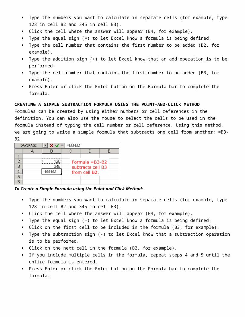
The result of a formula-the answer to 2+3, for example-displays in the cell on the Excel worksheet. The formula is visible only in the formula bar. A formula's result will change as different numbers are entered into the cells included in the formula's definition.

CREATING A SIMPLE ADDITION FORMULAA simple formula in Excel contains one mathematical operation only: one number plus a second number equals a third number. Writing a simple formula is really no more difficult than that: 1+1. The only difference in Excel is that all formulas must begin with the equal sign (=). It is not enough to type 1+1 in Excel because what will appear in the cell is "1+1." You must begin the equation with an equal sign, or =1+1. This holds true for any formula, simple or complicated, that adds, subtracts, multiplies or divides.

Let's add two numbers to create a third, 128+345=473. In Excel, this would be expressed by the formula, =128+345, as shown below.

Formulas begin with =

To Create a Simple Formula that Adds Two Numbers:

Click the cell where the formula will be defined. Type the equal sign (=) to let Excel know a formula is being defined. Type the first number to be added (128, for example) Type the addition sign (+) to let Excel know that an add operation is to be performed. Type the second number to be added (345, for example Press Enter or click the Enter button on the Formula bar to complete the formula.

But what if a column contains many numbers, each of which regularly changes? You don't want to write a new formula each time a number is changed. Luckily, Excel XP lets you include cell references in formulas.

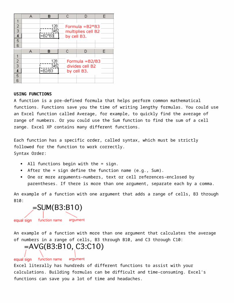
A formula can add the value of two cells-B2 and B3, for example. Type any two values in these two cells and the formula will adjust the answer accordingly.

Using this method to calculate two numbers-128 and 345, for example-requires that you type 128 in cell B2, for example, and 345 in cell B3. The Excel formula, =B2+B3, would then be defined in cell B4.

To Create a Simple Formula that Adds the Contents of Two Cells:

Type the numbers you want to calculate in separate cells (for example, type 128 in cell B2 and 345 in cell B3). Click the cell where the answer will appear (B4, for example). Type the equal sign (=) to let Excel know a formula is being defined. Type the cell number that contains the first number to be added (B2, for example). Type the addition sign (+) to let Excel know that an add operation is to be performed. Type the cell number that contains the first number to be added (B3, for example). Press Enter or click the Enter button on the Formula bar to complete the formula.

CREATING A SIMPLE SUBTRACTION FORMULA USING THE POINT-AND-CLICK METHODFormulas can be created by using either numbers or cell references in the definition. You can also use the mouse to select the cells to be used in the formula instead of typing the cell number or cell reference. Using this method, we are going to write a simple formula that subtracts one cell from another: =B3-B2.

To Create a Simple Formula using the Point and Click Method:

Type the numbers you want to calculate in separate cells (for example, type 128 in cell B2 and 345 in cell B3). Click the cell where the answer will appear (B4, for example). Type the equal sign (=) to let Excel know a formula is being defined. Click on the first cell to be included in the formula (B3, for example). Type the subtraction sign (-) to let Excel know that a subtraction operation is to be performed. Click on the next cell in the formula (B2, for example). If you include multiple cells in the formula, repeat steps 4 and 5 until the entire formula is entered. Press Enter or click the Enter button on the Formula bar to complete the formula.

USING FUNCTIONSA function is a pre-defined formula that helps perform common mathematical functions. Functions save you the time of writing lengthy formulas. You could use an Excel function called Average, for example, to quickly find the average of range of numbers. Or you could use the Sum function to find the sum of a cell range. Excel XP contains many different functions.

Each function has a specific order, called syntax, which must be strictly followed for the function to work correctly.Syntax Order:

All functions begin with the = sign. After the = sign define the function name (e.g., Sum).

One or more arguments-numbers, text or cell references-enclosed by parentheses. If there is more than one argument, separate each by a comma.

An example of a function with one argument that adds a range of cells, B3 through B10:

An example of a function with more than one argument that calculates the average of numbers in a range of cells, B3 through B10, and C3 through C10:

Excel literally has hundreds of different functions to assist with your calculations. Building formulas can be difficult and time-consuming. Excel's functions can save you a lot of time and headaches.

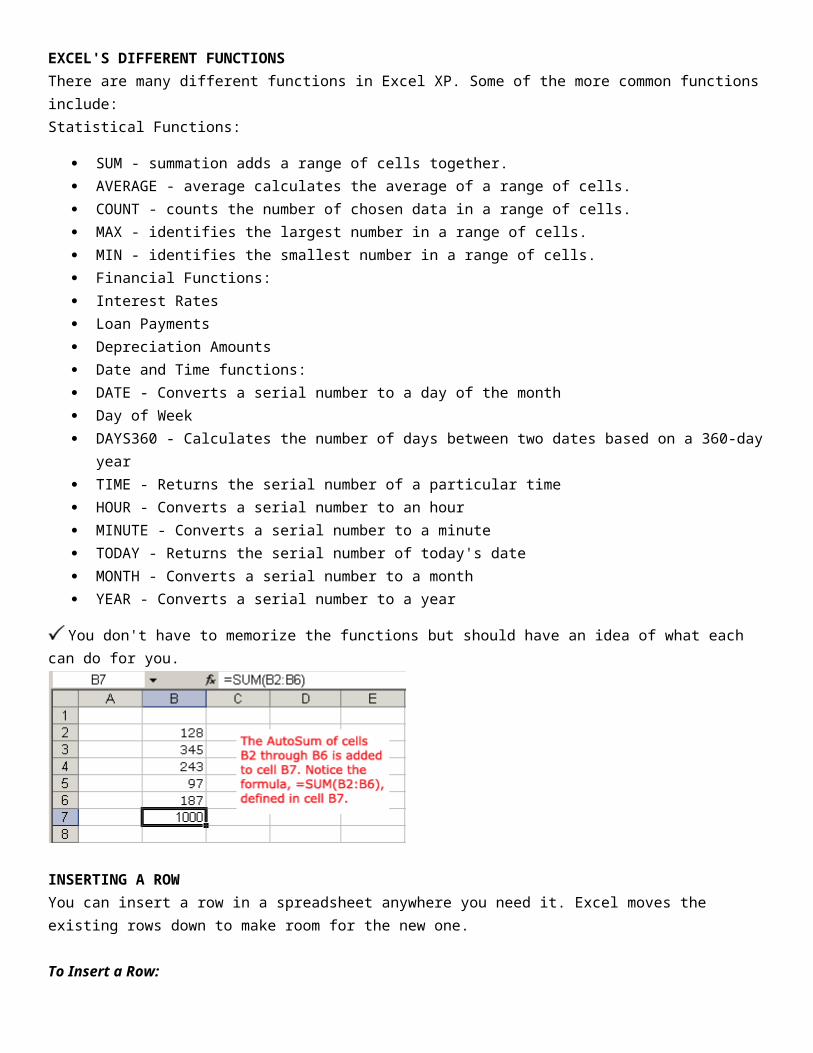
EXCEL'S DIFFERENT FUNCTIONSThere are many different functions in Excel XP. Some of the more common functions include:Statistical Functions:

SUM - summation adds a range of cells together. AVERAGE - average calculates the average of a range of cells. COUNT - counts the number of chosen data in a range of cells. MAX - identifies the largest number in a range of cells. MIN - identifies the smallest number in a range of cells. Financial Functions: Interest Rates Loan Payments Depreciation Amounts Date and Time functions: DATE - Converts a serial number to a day of the month Day of Week DAYS360 - Calculates the number of days between two dates based on a 360-day year TIME - Returns the serial number of a particular time HOUR - Converts a serial number to an hour MINUTE - Converts a serial number to a minute TODAY - Returns the serial number of today's date MONTH - Converts a serial number to a month YEAR - Converts a serial number to a year

You don't have to memorize the functions but should have an idea of what each can do for you.

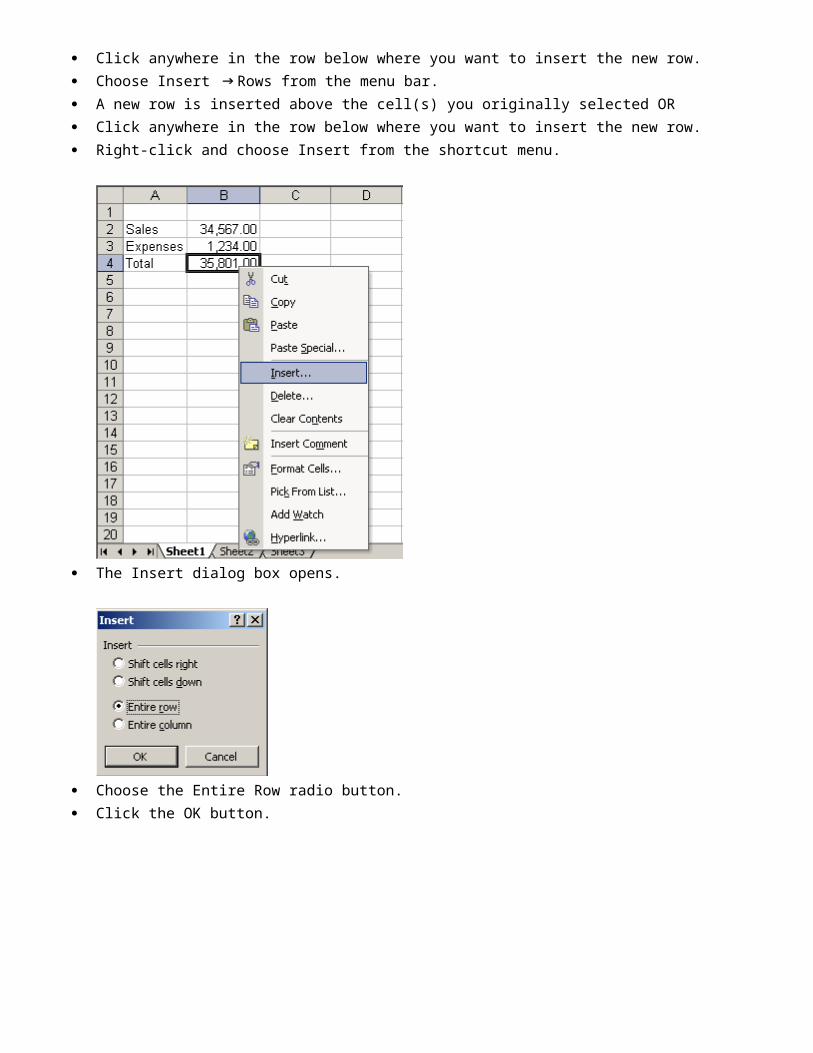
INSERTING A ROWYou can insert a row in a spreadsheet anywhere you need it. Excel moves the existing rows down to make room for the new one.

To Insert a Row:

Click anywhere in the row below where you want to insert the new row. Choose Insert Rows from the menu bar. A new row is inserted above the cell(s) you originally selected OR Click anywhere in the row below where you want to insert the new row. Right-click and choose Insert from the shortcut menu.

The Insert dialog box opens.

Choose the Entire Row radio button. Click the OK button. A new row is inserted above the cell(s) you originally selected.

Select multiple rows before choosing Insert to add rows quickly. Excel inserts the same number of new rows that you originally selected.

ADJUSTING COLUMN WIDTHSBy default, Excel's columns are 8.43 characters wide, but each individual column can be enlarged to 240 characters wide.If the data being entered in a cell is wider or narrower than the default column width, you can adjust the column width so it is wide enough to contain the data.

You can adjust column width manually or use AutoFit.

To Manually Adjust a Column Width:

Place your mouse pointer to the right side of the gray column header.

###

The mouse pointer changes to the adjustment tool (double-headed arrow).

Drag the Adjustment tool left or right to the desired width and release the mouse button.

To AutoFit the Column Width:

Place your mouse pointer to the right side of the column header. The mouse pointer changes to the adjustment tool (double-headed arrow). Double-click the column header border.

Excel "AutoFits" the column, making the entire column slightly larger than the largest entry contained in it.To access AutoFit from the menu bar, choose Format Column AutoFit Selection.

ADJUSTING ROW HEIGHTChanging the row height is very much like adjusting a column width. There will be times when you want to enlarge a row to visually provide some space between it and another row above or below it.

To Adjust Row Height of a Single Row:

Place your mouse pointer to the lower edge of the row heading you want to adjust. The mouse pointer changes to the adjustment tool (double-headed arrow).

Drag the Adjustment tool up or down to the desired height and release the mouse button.

To AutoFit the Row Height:

Place your mouse pointer to the lower edge of the row heading you want to adjust. The mouse pointer changes to the adjustment tool (double-headed arrow). Double-click to adjust the row height to "AutoFit" the font size.

Excel XP "AutoFits" the row, making the entire row slightly larger than the largest entry contained in the row.

UNDERSTANDING THE DIFFERENT CHART TYPESExcel XP allows you to create many different kinds of charts.

Area ChartAn area chart emphasizes the trend of each value over time. An area chart also shows the relationship of parts to a whole.

Column ChartA column chart uses vertical bars or columns to display values over different categories. They are excellent at showing variations in value over time.

Bar ChartA bar chart is similar to a column chart except these use horizontal instead of vertical bars. Like the column chart, the bar chart shows variations in value over time.

Line ChartA line chart shows trends and variations in data over time. A line chart displays a series of points that are connected over time.

Pie ChartA pie chart displays the contribution of each value to the total. Pie charts are a very effective way to display information when you want to represent different parts of the whole, or the percentages of a total.

Other ChartsOther charts that can be created in Excel XP include: Doughnut; Stock XY (scatter); Bubble; Radar; Surface; or Cone, Cylinder, and Pyramid charts.

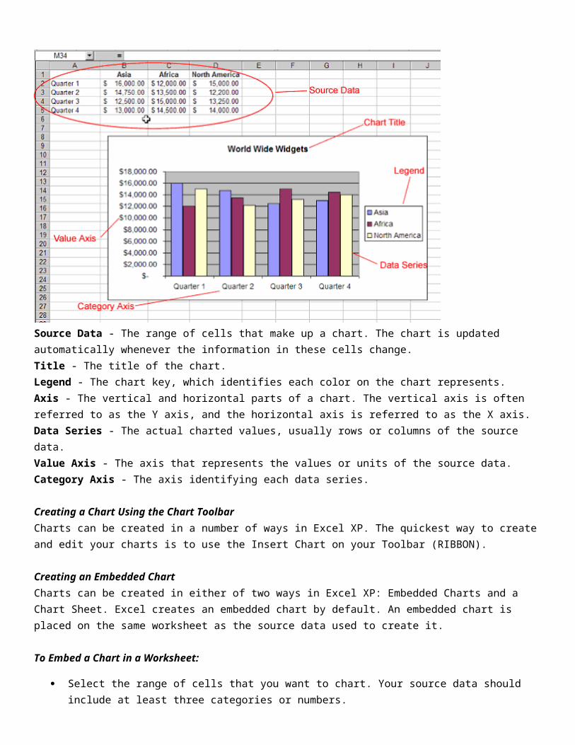
Identifying the Parts of a ChartHave you ever read something you didn't fully understand but when you saw a chart or graph, the concept became clear and understandable? Charts are a visual representation of data in a worksheet. Charts make it easy to see comparisons, patterns, and trends in the data.

Source Data - The range of cells that make up a chart. The chart is updated automatically whenever the information in these cells change.Title - The title of the chart.Legend - The chart key, which identifies each color on the chart represents.Axis - The vertical and horizontal parts of a chart. The vertical axis is often referred to as the Y axis, and the horizontal axis is referred to as the X axis.Data Series - The actual charted values, usually rows or columns of the source data.Value Axis - The axis that represents the values or units of the source data.Category Axis - The axis identifying each data series.

Creating a Chart Using the Chart ToolbarCharts can be created in a number of ways in Excel XP. The quickest way to create and edit your charts is to use the Insert Chart on your Toolbar (RIBBON).

Creating an Embedded ChartCharts can be created in either of two ways in Excel XP: Embedded Charts and a Chart Sheet. Excel creates an embedded chart by default. An embedded chart is placed on the same worksheet as the source data used to create it.

To Embed a Chart in a Worksheet:

Select the range of cells that you want to chart. Your source data should include at least three categories or numbers.

Choose Insert on the menu bar. Select the type of Chart you wish to insert.

Different charts work best with different data. A pie chart, for example, can only display one data series at a time.

PRINTING A WORKSHEET OR WORKBOOKPrinting in Excel is much like printing in other Office applications like Microsoft Word. As previously mentioned, Excel defaults to printing the entire worksheet.To Print a Worksheet:

Choose File Print from the menu bar. The Print dialog box opens.

Specify the Printer Name where the spreadsheet will print. If you only have one printer in your home or office, Excel will default to that printer.

Choose whether to print All or a certain range of pages

Choose the Number of Copies to print by clicking on the up or down arrows. Click the OK button to print the worksheet.

Don't print your Excel spreadsheet without checking spelling first! Excel includes two tools to help correct spelling errors: AutoCorrect and Spelling.