lec 07 transforms and quantization ii - university of …l.web.umkc.edu/.../notes/lec07.pdflec 07...

CS/EE 5590 / ENG 401 Special Topics (17804, 17815, 17803)

Lec 07

Transforms and Quantization II

Zhu Li

Course Web:

http://l.web.umkc.edu/lizhu/teaching/2016sp.video-communication/main.html

Z. Li Multimedia Communciation, 2016 Spring p.1

Outline

Lecture 06 Re-Cap

Scalar Quantization

Vector Quantization


Unitary Transforms

y=Ax, x,y in Rd, A: dxd

Unitary Transforms: A is unitary if: A-1=AT, AAT = Id

The basis of A is orthogonal to each other

Examples:


y x= A=

[a1T, a2T ,…, adT]

� = ��

�

��

Inner product<x, ak>

�< ��, �� >= 0< �� , �� >= 1

cossin

sincos

2

1

2

12

1

2

1

21

32

Unitary Transform Properties

Preserve Energy:

Preserve Angles:

DoF of Unitary Transforms k-dimension projections in d-dimensional space: kd – k2. Above example: 3x2-2x2 = 2; normal points to the unit sphere


� = ��

��= ��

�= �� = �� = �� = �

�

�� = � ��= �

�

the angles between vectors are preserved

unitary transform: rotate a vector in Rn, i.e., rotate the basis coordinates

n

Energy Compaction and De-correlationEnergy Compaction

Many common unitary transforms tend to pack a large fraction of signal energy into just a few transform coefficients

De-correlation Highly correlated input elements quite uncorrelated output coefficients Covariance matrix

DCT Example: y=DCT(x), Question: Is there an optimal transform that do best in this ?

display scale: log(1+abs(g))

linear display scale: g

x: columns of image pixels

�� = �� = �{ � − � � � − �{�} �}

x1,x2,…, x600Rxx y1,y2,…, y600

Ryy

Karhunen-Loève Transform (KLT)

a unitary transform with the basis vectors in A being the “orthonormalized” eigenvectors of Rxx

assume real input, write AT instead of AH

denote the inverse transform matrix as A, AAT=I Rx is symmetric for real input, Hermitian for complex input

i.e. RxT=Rx, Rx

H = Rx

Rx nonnegative definite, i.e. has real non-negative eigen values

Attributions Kari Karhunen 1947, Michel Loève 1948 a.k.a Hotelling transform (Harold Hotelling, discrete formulation 1933) a.k.a. Principle Component Analysis (PCA, estimate Rx from samples)

� = ��, � = ��AT = [a1, a2, …, ad]

�� = �� , � = 1, 2, … ,�

Decorrelation by construction:

Minimizing Error under limited coefficients reconstruction

Properties of K-L Transform

Basis restriction: Keep only a subset of m transform coefficients and then perform inverse transform (1 m N)

Keep the coefficients w.r.t. the eigenvectors of the first m largest eigenvalues (indication of energy)

�� = �{��} = � �� = ��=

��

��

�� = �

0, ��! = �� , �� = �

Energy Compaction Comparison

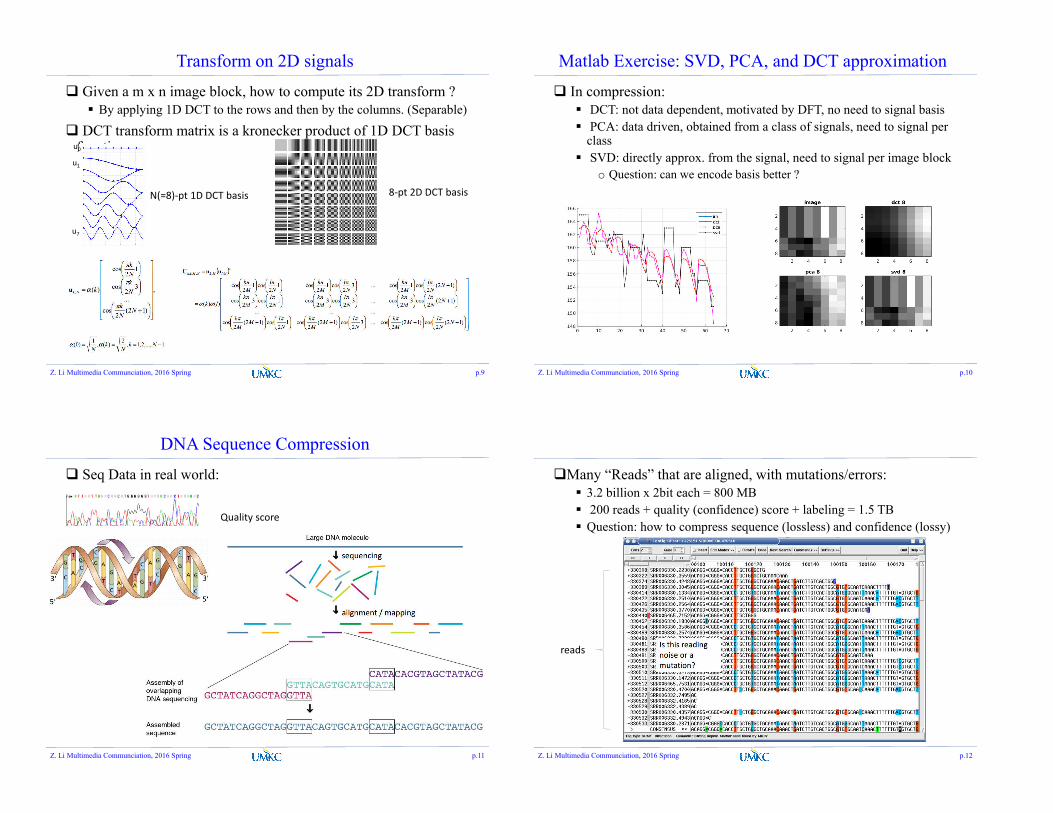
Transform on 2D signals

Given a m x n image block, how to compute its 2D transform ? By applying 1D DCT to the rows and then by the columns. (Separable)

DCT transform matrix is a kronecker product of 1D DCT basis function


u0

u7

u1

N(=8)-pt 1D DCT basis 8-pt 2D DCT basis

Matlab Exercise: SVD, PCA, and DCT approximation

In compression: DCT: not data dependent, motivated by DFT, no need to signal basis PCA: data driven, obtained from a class of signals, need to signal per

class SVD: directly approx. from the signal, need to signal per image block

o Question: can we encode basis better ?


DNA Sequence Compression

Seq Data in real world:


Quality score

Many “Reads” that are aligned, with mutations/errors: 3.2 billion x 2bit each = 800 MB 200 reads + quality (confidence) score + labeling = 1.5 TB Question: how to compress sequence (lossless) and confidence (lossy)


reads

FastQ and SAM

Current solutions: Reminds of zigzag and run-level coding…


Outline

Lecture 06 Re-Cap

Scalar Quantization Uniform Quantization Non-Uniform Quantizatoin

Vector Quantization


Rate Distortion Encoder and Decoder

Decoder: Map fn(Xn) to a reconstruction sequence.

Scalar quantizer: n = 1, quantize each sample individually.

Vector quantizer: n > 1, quantize a group of samples jointly.

EncoderXn

Decoder nX̂ 2 ..., ,2 ,1 )( nRn

n Xf

Encoder: Represent a sequence Xn = {X1, X2, …, Xn} by an indexfn(Xn) in {1, 2, …, 2nR}.

Z. Li, Multimedia Communciation, 2016 Spring p.15

Scalar Quantization

b4b3b2b1b0=-∞ b5 b6 b7 b8=∞

y4y3y2y1 y5 y6 y7 y8 x

Encoder: Partition the real line into M disjoint intervals:

1.-M ..., 1, 0, i ),,[ 1 iii bbI

.......00 Mbbb

Ii: Quantization bins.

i: Index of quantization bin.

bi: Decision boundaries.

yi: Reconstruction levels.

Encoder: sends the code word of each interval/bin index to the decoder.

Decoder: represents all values in an interval by a reconstruction level.

Fixed len Code: 000 001 010 011 100 101 110 111


Rate-Distortion Tradeoff

Things to be determined: Number of bins Decision boundaries Reconstruction levels Codewords for bin indexes.

The design of quantization is a tradeoff between rate and distortion:To reduce the size of the encoded bits, we need

to reduce the number of bins More distortions

The performance is governed by the rate-distortion theory

Rate

Distortion

A

B


Model of Quantization

Quantization: q = A(x): map x to an index

Inverse Quantization: )())(()(ˆ xQxABqBx B(x) is not exactly the inverse function of A(x), because xx ˆ

xxxe ˆ)(Quantization error:

Aq

x̂x B

Q x̂x

Combining quantizer and de-quantizer:e(x)

x̂xor


Measure of Distortion

Quantization error:

Mean Squared Error (MSE) for Quantization Average quantization error of all input values Need to know the probability distribution of the input

Number of bins: M

Decision boundaries: bi, i = 0, …, M

Reconstruction Levels: yi, i = 1, …, M

Reconstruction: iii bxbyx 1 iff ˆ

M

i

b

b

i

i

i

dxxfxydxxfxxMSEd1

22

1

)()(ˆ

xxxe ˆ)(

b4b3b2b1b0 b5 b6 b7 b8

y4y3y2y1 y5 y6 y7 y8 x


Uniform Midrise Quantizer

All bins have the same size except possibly for the two outer intervals: bi and yi are spaced evenly The spacing of bi and yi are both ∆ (step size)

∆ 2∆ 3∆ Input

-3∆ -2∆ -∆

Reconstruction3.5∆

2.5∆

1.5∆0.5 ∆

-0.5∆

-1.5∆

-2.5∆-3.5∆

Uniform Midrise Quantizer

Even number of recon levels0 is not a recon level

iii bby 12

1for inner intervals.

x0-∆ ∆-2∆ 2∆-3∆ 3∆

-xmax xmax

x0-∆ ∆-2∆ 2∆

Xmin=-∞ xmax=∞

For finite Xmax and Xmin:

For infinite Xmax and Xmin:

The two outer-most recon levelsare still one step size away from the inner ones.

6 bins

6 bins


Uniform Midtread Quantizer

-2.5∆ -1.5∆ -0.5∆

Reconstruction3∆

2∆

∆

-∆

-2∆-3∆


0.5∆ 1.5∆ 2.5∆ Input

- Odd number of recon levels- 0 is a recon level- Desired in image/video coding

x0-0.5∆ 0.5∆-1.5∆ 1.5∆-2.5∆ 2.5∆

-xmax xmax

Xmin=-∞ xmax=∞

For finite Xmax and Xmin:

For infinite Xmax and Xmin:

5 bins

x0-0.5∆ 0.5∆-1.5∆ 1.5∆

5 bins



5.0)()(

xxsignxAq

Quantization mapping:

Output is an index

Example:

x = 1.8∆, q = 2.

-2.5∆ -1.5∆ -0.5∆

Reconstruction

3∆

2∆

∆

-∆

-2∆

-3∆

0.5∆ 1.5∆ 2.5∆ Input

qqBx )(ˆ

De-quantization mapping:

Example:

q = 2 2x̂

x0-0.5∆ 0.5∆-1.5∆ 1.5∆-2.5∆ 2.5∆


Quantization of a Uniformly Distributed Source

Input X: uniformly distributed in [-Xmax, Xmax]: f(x)= 1 / (2 Xmax)

Number of bins: M (even for midrise quantizer)

Step size: ∆ = 2 Xmax / M.

b40

b3-∆

b2-2∆

b1-3∆

b0-4∆

b5∆

b62∆

b73∆

b84∆

-Xmax Xmax

y4-0.5 ∆

y3-1.5∆

y2-2.5∆

y1-3.5∆

y50. 5∆

y61.5∆

y72.5∆

y83.5∆ x

is uniformly distributed in [-∆/2, ∆/2].

x0.5 ∆

-0.5 ∆

∆ 2∆ 3∆ 4∆-∆-2∆-3∆-4∆

xxxe ˆ)(


Quantization of a Uniformly Distributed Source

MSE

2

12

1d

How to choose M, the number of bins, such that the distortion is less than a desired level D?

DXMD

M

XD

3

1

2

12

1

12

1max

2

max2

M

i

b

b

i

i

i

dxxfxydxxfxxd1

22

1

)()(ˆ

Prove that

Proof: The pdf is 1

( )f xM

2 3 2

0

1 1 1 1/ 2

12 12d M x dx

M


Signal to Noise Ratio (SNR)

Let M = 2R, each bin index can be represented by R bits.

dBR

RMMX

X

X

EnergyNoise

nergySignaldBSNR

R

02.6

)2log20(2log10log10/2

2log10

12/1

212/1log10

E log10)(

102

102

102max

2max

10

2

2max

1010

Variance of a random variable uniformly distributed in [- L/2, L/2]:

22/

2/

22

12

110 Ldx

Lx

L

L

x


�� = 10 log��

��= 10 log��

255�

��

Outline

Lecture 06 Re-Cap

Scalar Quantization Uniform Quantization Non-Uniform Quantization

Vector Quantization


Non-uniform Quantization

Uniform quantizer is not optimal if source is not uniformly distributed

For given M, to reduce MSE, we want narrow bin when f(x) is high and wide bin when f(x) is low

x

f(x)

0

M

k

b

b

k

k

k

dxxfxydxxfxxd1

22

1

)()(ˆ


Lloyd-Max Scalar Quantizer

Also known as pdf-optimized quantizer

Given M, the optimal bi and yi that minimize MSE satisfy:

.0 ,0 :condition Lagrangian

ii b

d

y

d

i

i

i

i

b

b

b

bii

i dxxf

dxxfx

IXXEyy

d

1

1

)(

)(

| 0

yi is the centroid of interval [b(i-1), b(i)].

(conditional mean)

x

f(x)

0 bi-1 bi

yi

M

k

b

b

k

k

k

dxxfxydxxfxxd1

22

1

)()(ˆ



2

0)()( 0

1

21

2

iii

iiiiiii

yyb

bfbybfbyb

d

bi is the midpoint of yi and yi+1

Nearest neighboring quantizer. x0 bi-1 bi bi+1

yi yi+1

i

i

i

i

b

b

b

bi

dxxf

dxxfx

y

1

1

)(

)(

Summary of Lloyd-Max conditions:

2 1 ii

i

yyb


A special case

Relationship to uniform quantizer: If f(x) = c (uniform), Lloyd-Max quantizer

reduces to uniform quantizer

)(2

1)(21

)(

)(

)(

11

21

2

1

1

1

1

ii

ii

ii

ii

b

b

b

b

b

bi bb

bb

bb

bbc

dxxc

dxxf

dxxfx

y

i

i

i

i

i

i

If the rate is high, f(x) is close to constant in each bin, we also have

L-M quantizer reduces to uniform quantizer.

2/)( 1 iii bby


Example

For the given pdf, design the optimal

2-level mid-rise quantizer.

Solution: By symmetry, b0 = -1, b1 = 0, b2 = 1.

x

f(x)

0 1 -1

1

1 1

0 01 1

0

( 1) ( 1)1/ 6

1/ 3.1/ 2 1/ 2

( )

x x dx x x dx

y

f x dx



How to find optimal bi and yi simultaneously? A deadlock:

o Reconstruction levels depend on decision levelso Decision levels depend on reconstruction levels

Solution: iterative method !

i

i

i

i

b

b

b

bi

dxxf

dxxfx

y

1

1

)(

)(

2

1 ii

i

yyb

Given bi, can find the corresponding optimal yi

Given yi, can find the corresponding optimal bi

Summary of conditions for optimal quantizer:


Lloyd Algorithm (with known f(x) )

If the pdf f(x) is known:

1. Initialize all yi, let j = 1, d0 = ∞ (distortion).

2. Update all decision levels

3. Update all yi,

4. Computer MSE:

5. If (dj-1 – dj) / dj-1 < ε, stop, otherwise set j = j + 1, go to step 2.

M

k

b

b

kj

k

k

dxxfyxd1

2

1

)(

2 1 ii

i

yyb

i

i

i

i

b

b

b

b

i dxxfdxxfxy11

)(/)(


Performance of Lloyd-Max Scalar QuantizerRecall: Upper & lower bounds for D(R) function:

RRx RDP 222 2)(2

)(22 2

1 Xhx e

P

: Entropy Power (always ≤ σ2)

Distribution Entropy Power

Uniform

Laplacian

Gaussian

22 703.0

6

e

22 865.0

e

2


Performance of Lloyd-Max Scalar QuantizerLet X take values in [-V, V] with pdf f(x) and variance ��. If X is quantized into M bins

by the Lloyd-Max quantizer, it can be shown that when M is large, the minimal MSE is

3

0

32

)(3

2

Vdxxf

Md

Significance: direct estimate of the quantization error in terms of the pdf and the number of bins.

Proof can be found in the following places:

Panter, Dite, Quantization Distortion in Pulse-Count Modulation with NonuniformSpacing of Levels, Proceedings of IRE, 1951.

Notes:

1. This is only good for finite range V.

2. The formula is exact for piecewise constant pdf.


Performance of Lloyd-Max Scalar Quantizer Rate-Distortion performance:

If M = 2^R RRVdxxfd 2222

3

0

3 22)(3

2

3

0

32

)(3

2

Vdxxf

Md

where .)(3

2 3

0

322

Vdxxf

Example: If X has uniform distribution in [-V, V], then

.1 3

1

2

1

3

2)(

3

2 22233

0

322

VV

Vdxxf

V

.12

12

32 22

2222 RR V

d

L-M quantizer reduces to uniform quant.Comparing with bounds: LM quantizer only achieves the upper bound.


Outline

Lecture 06 Re-Cap

Scalar Quantization

Vector Quantization


Vector Quantization

EncoderXn

Decoder nX̂ 2 ..., ,2 ,1 )( nRn

n Xf

Encoder: Represent a sequence Xn = {X1, X2, …, Xn} by an index

fn(Xn) in {1, 2, …, 2nR}. Decoder: Map fn(Xn) to a reconstruction sequence (codeword).

Codebook: the collection of all codewords.

Questions to be addressed: Why this is better than scalar quantizer? How to generate the codebook? How to find the best codeword for each input block?


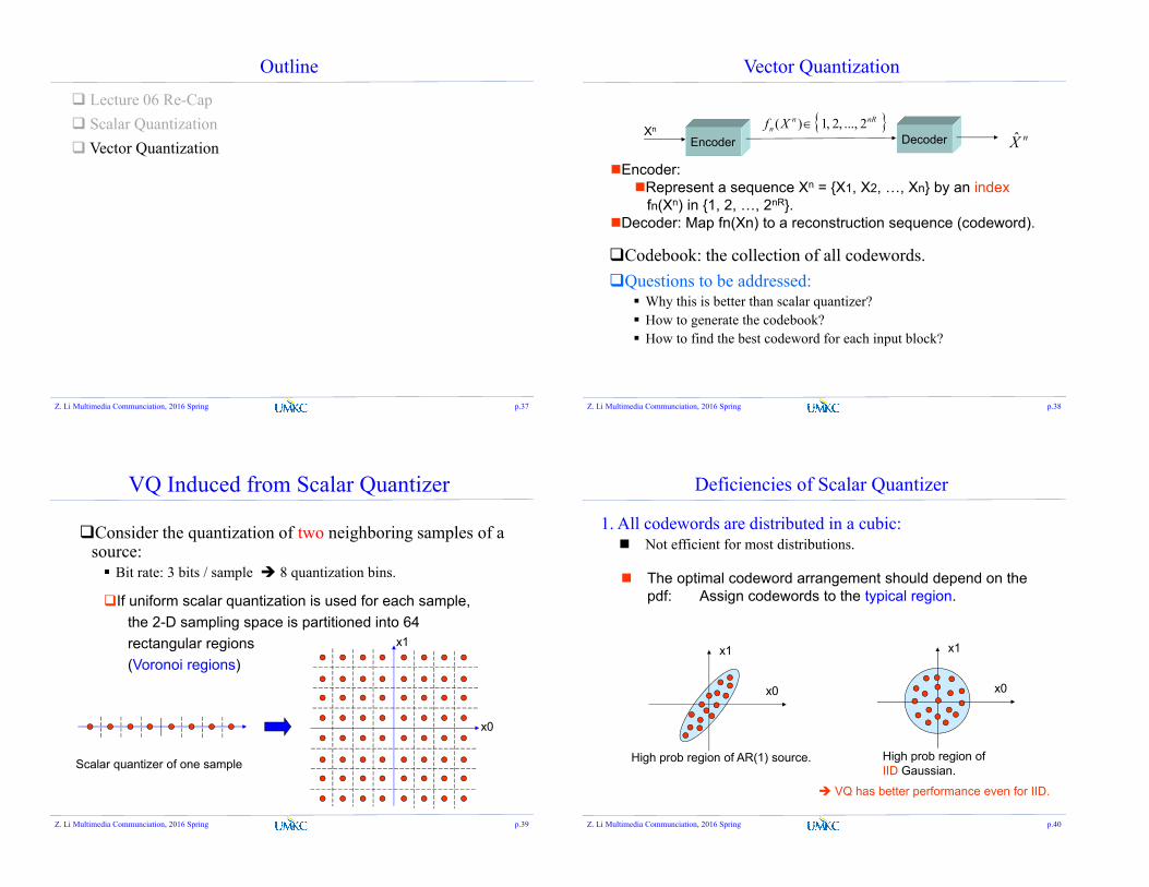
VQ Induced from Scalar Quantizer

Consider the quantization of two neighboring samples of a source: Bit rate: 3 bits / sample 8 quantization bins.

Scalar quantizer of one sample

x0

x1

If uniform scalar quantization is used for each sample,

the 2-D sampling space is partitioned into 64

rectangular regions

(Voronoi regions)


x0

x1

High prob region of IID Gaussian.

VQ has better performance even for IID.

Deficiencies of Scalar Quantizer

1. All codewords are distributed in a cubic: Not efficient for most distributions.

x0

x1

High prob region of AR(1) source.

The optimal codeword arrangement should depend on the pdf: Assign codewords to the typical region.


Deficiencies of Scalar Quantizer

2. The Voronoi regions induced from SQ are always cubic:

Cubic region vs spherical region: Given the same volume, the granular error of the sphere is the smallest

among different shapes.

.42.16

lim spherespherecubic

n

MSEMSEe

MSE

or 1.53 dB loss for cubic Voronoi regions (same for all pdfs).

Given the same volumes (i.e., rate R), the MSE of the

spherical Voronoi region is the minimum among all shapes:

Area: 1Side length: 1Max error: 0.707

Area: 1Radius=Max error:

56.0/1


Linde-Buzo-Gray (LBG) Algorithm

Algorithm to select code-words from a training set.

Also known as Generalized Lloyd Algorithm (GLA):1. Start from an initial set of recon values {yi}, i=1 to M, and a set

of training vectors {Xn}, n = 1, … N.2. For each training vector Xn, find the recon value that is closest to

it.Q(Xn)= Yj iff d(Xn, Yj) ≤ d(Xn, Yi) for all i ≠ j.

3. Compute average distortion.4. If distortion is small enough, stop.

Otherwise, replace the recon value by the avg values of all vectorsin each quantization region. Go to Step 2.


Matlab Implementation

kmeans() % desired rate R=8; [indx, vq_codebook]=kmeans(x, 2^R);

kd-tree implementation [kdt.indx, kdt.leafs, kdt.mbox]=buildVisualWordList(x, 2^R); [node, prefix_code]=searchVisualWordList(q, kdt.indx, kdt.leafs);


Summary

Transforms Unitary transform preserves energy, angle, limited DoF KLT/PCA: energy compaction and de-correlation DCT: a good KLT/PCA approximation A bit of intro to Genome Info Compression, more to come

Scalar Quantization: If signal is uniform, what is the expected quantization error ? Non-uniform signal distribution, optimal quantization design (Lloyd-

Max)

Vector Quantization: More efficient Fast algorithm exists like kd-tree based A special case of transform: over-complete basis, very sparse

coefficient (only 1 none zero entry) Shall revisit with coupled dictionary approach in super resolution


lec 07 transforms and quantization ii - university of …l.web.umkc.edu/.../notes/lec07.pdflec 07...

Documents