AY216 1

Lec. 4 Heating and Coolingand

Line Diagnostics for HII Regions

References: Spitzer, Ch. 6 Osterbrock & Ferland Ch. 3-6Tielens, Chs. 3 & 4McKee, ay216_2006_05_HIIThernal.pdf

1. General Theory of Heating & Cooling2. Line Cooling Function3. Cooling of HII Regions4. Diagnostics of HII Regions

AY216 2

The First Law of Thermodynamics for fluids is

The Heat Equation

The so far incorrect treatment of the temperature of HIIregions requires a more general development of heatingand cooling. This is done by including thermodynamics inthe equations of hydrodynamics (or MHD) which expressthe conservation laws for fluids, in this case the ISM.

Tds = de pd(1/ )where s and e are the entropy and energy per unit mass, is themass density per unit volume, and p is the pressure; e is the sumover all constituents of kinetic, internal (excitation) and chemical(including ionization) energies:

e = ekin + eex + echemFor example, the chemical energy of an H+ ion is 13.6eV and of an H2 molecule is -4.48eV. We ignore the chemical energy and combine the first two terms into a combined thermal energy.

AY216 3

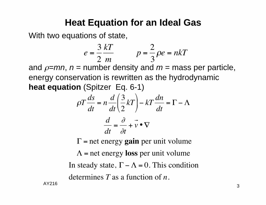
Heat Equation for an Ideal Gas

With two equations of state,

e =3

2

kT

m p =

2

3e = nkT

and =mn, n = number density and m = mass per particle,energy conservation is rewritten as the hydrodynamicheat equation (Spitzer Eq. 6-1)

Tds

dt= n

d

dt

3

2kT

kT

dn

dt=

d

dt=

t+ v •

= net energy gain per unit volume

= net energy loss per unit volume

In steady state, = 0. This condition

determines T as a function of n.

AY216 4

Heat Equation for a Molecular Gas

We can generalize the treatment for point molecules to molecular gases by writing the energy as

e =1

1

p

where is the ratio of specific heats (5/3 for point molecules, 7/5 fordiatomic molecules, etc.), This form supposes thermal equilibrium,which may not apply to interstellar gases. For example, the mostabundant interstellar molecule is H2 , whose rotational levels havelarge excitation energies and are not fully thermalized.

p

1

d

dtln

p

=

By recognizing that p/ = c2= kT/m, where c is the isothermalsound speed, the heat equation can be manipulated Into the form,

Thus = requires adiabatic changes: p

AY216 5

Heating Processes

A heating process increases the thermal (mean kinetic)energy of the gas. This can only happen by particlecollisions with some non-thermal component. Wemay think of this component external to the gas.

1. Photons - In ionizing or dissociating the gas, a suprathermalparticle is produced, e.g., a photoelectron or a dissociated H atom,that heats the gas on collisions with ambient thermal particles.Usually the photons are in the UV to X-ray bands. Photoelectricheating may also be generated by photons absorbed by dustparticles or large molecules such as PAHS.

2. Cosmic rays - High energy particles ( > 1 MeV) slow downby ionizing and exciting H and He (and by direct collisionswith ambient electrons). The ejected fast electrons heat the gasby collisions.

3. Dust-Gas Interaction - Collisions between gas and dustexchange energy, and heat the gas (cool) when the dust iswarmer (cooler) than the gas.

AY216 6

Heating Mechanisms (cont’d)

5. Magnetic Heating - Reconnection and ambipolar-diffusion (ion-neutral collisions as fields slip through neutral gas.

4. Mechanical Heating - Dissipation in shocks and turbulence

Further Preliminary Comments on Heating:• Photoelectric heating is the best understood. Heating of HII regions is the prototypical case, as discussed in Lecture 3.• Cosmic ray heating is uncertain because of ignorance about the low-energy spectrum and MHD transport.• Dust-Gas heating is reasonably well understood, although it depends on dust properties (abundance, size, surface).• Mechanical heating is usually treated phenomenologically.• Shock heating is affected by the detailed properties of shocks.

Heating processes will be discussed later in more detail,e.g., in Lec07; see also McKee’s lecture, ay216_2006_05.

AY216 7

Cooling Processes

In contrast to the diversity (and uncertainty) of heating processes, cooling of interstellar gas is mainly by radiation, especially lines.

1. Line Radiation - Thermal particle energy is expended in exciting atoms and molecules, whose re-radiation cools the gas if it escapes. This is the main topic of this lecture.

2. Continuum Radiation - One example already encountered in recombination cooling, where the recombination of the particles isaccompanied by a continuum photon. Another example is free-free radiation or bremsstrahlung, which generates far-IR andradio continuum by HII regions, but plays a small role in cooling.

3. Dust-Gas Collisional Energy Exchange- This leads to gas cooling when the dust is cooler than the gas.

4. Expansion Cooling - This form of mechanical cooling occurs when the gas (cloud or wind) expands, in analogy to “adiabaticcooling”.

AY216 8

is the net rate at which energy is lost incollisions. (For HII regions, electrons arethe most important collision partners.)The collisions are described by upwardand downward rate coefficients klu & kul,

related by detailed balance.

NB Instead of j and k for lower

and upper levels, we use u and l

2. Line Cooling Function

----------------------- IP

______________ u ex de-ex______________ l

----------------------- ground “Atom“A

c + Al Au + c

E c = Ec Eul

kul

= v lu kul = v lu

glklu = gukuleEul / kT

The net cooling per unit volume (Spitzer Eq. 6-5) is

= nc (nlklu nukul )Eul

ul

NB: If the levels are exactly in thermal equilibrium, =0!

AY216 9

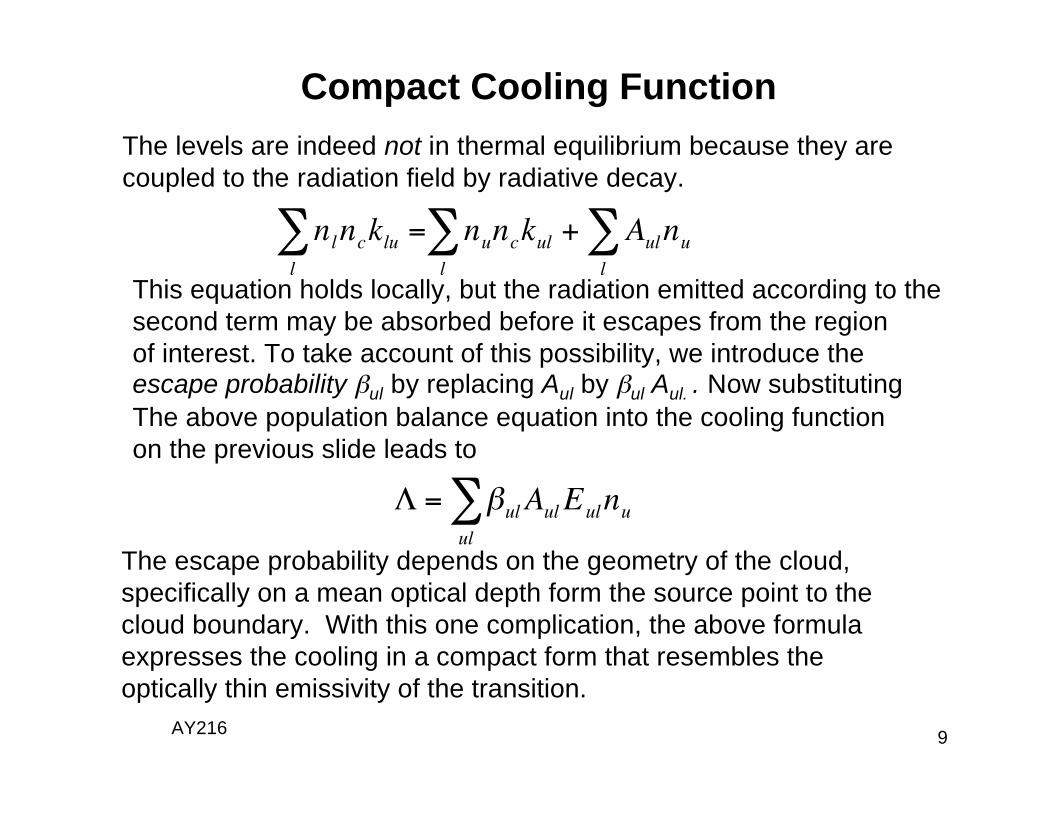
Compact Cooling Function

The levels are indeed not in thermal equilibrium because they are coupled to the radiation field by radiative decay.

nlncklu =l

nunckul + Aulnull

This equation holds locally, but the radiation emitted according to thesecond term may be absorbed before it escapes from the region of interest. To take account of this possibility, we introduce theescape probability ul by replacing Aul by ul Aul. . Now substitutingThe above population balance equation into the cooling functionon the previous slide leads to

= ul AulEul

ul

nu

The escape probability depends on the geometry of the cloud, specifically on a mean optical depth form the source point to thecloud boundary. With this one complication, the above formula expresses the cooling in a compact form that resembles the optically thin emissivity of the transition.

AY216 10

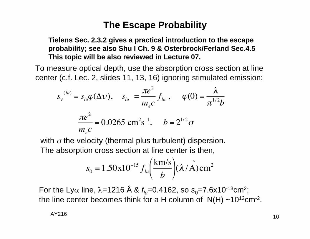
The Escape Probability

Tielens Sec. 2.3.2 gives a practical introduction to the escape

probability; see also Shu I Ch. 9 & Osterbrock/Ferland Sec.4.5

This topic will be also reviewed in Lecture 07.

To measure optical depth, use the absorption cross section at linecenter (c.f. Lec. 2, slides 11, 13, 16) ignoring stimulated emission:

s (lu)= slu ( ), slu =

e2

mecflu , (0) = 1/ 2b

e2

mec= 0.0265 cm2s 1, b = 21/ 2

with the velocity (thermal plus turbulent) dispersion.The absorption cross section at line center is then,

s0 =1.50x10 15 flukm/s

b

( /A)

o

cm2

For the Ly line, =1216 Å & flu=0.4162, so s0=7.6x10-13cm2;the line center becomes think for a H column of N(H) ~1012cm-2.

AY216 11

This exactly solvable model (using escape probability) illustratesbasic elements of radiative cooling and introduces the concept ofcritical density.The steady balance equation is

Model Two-Level System

________________ u

Aul Clu Cul

________________ l( ul Aul + Cul )nu = Clu(n nu),

n = nl + nu Cul = nckul , etc.

The population of the upper level is then

nun

=Clu

ul Aul + Cul + Clu

=

gugle Eul / kT

1+gugle Eul / kT + ul Aul

nckulafter dividing the first form by Cul and applying detailed balance

Clu

Cul

=klukul

=gugle Eul / kT

AY216 12

Two-Level Cooling Formula

nun

=Clu

ul Aul + Cul + Clu

=

gugle Eul / kT

1+gugle Eul / kT +

ncritnc

The third term of the denominator of the population of the upperlevel suggests introducing the critical density

ncrit = ul Aul

kulso that

and the cooling rate is

Lul = ul AulnuEul

gugle Eul / kT

1+gugle Eul / kT

+ncritnc

There are two simple limits:

nc << ncrit (subthermal) : Lul = kluncnEul

nc >> ncrit (thermalized) : Lul = ul AulnEul gu /gl e

Eul / kT

1+ gu /gl eEul / kT

AY216 13

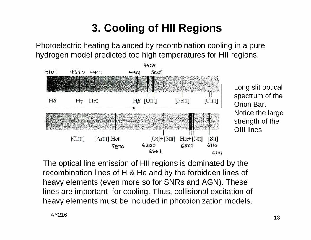
3. Cooling of HII Regions

Photoelectric heating balanced by recombination cooling in a purehydrogen model predicted too high temperatures for HII regions.

The optical line emission of HII regions is dominated by therecombination lines of H & He and by the forbidden lines ofheavy elements (even more so for SNRs and AGN). Theselines are important for cooling. Thus, collisional excitation ofheavy elements must be included in photoionization models.

Long slit optical spectrum of the Orion Bar.Notice the largestrength of the OIII lines

AY216 14

Historical Note on Nebular Lines

Helium – discovered in 1868 by Janssen in solar chromosphere (in eclipse) at5816 Angstroms.

Identified as non-terrestrial by Lockyer & Franklund; later detected in minerals.

Significance: 40% of the visible mass had been missed (although the fact thatmost of it is hydrogen was unknown then).

Nebulium – discovered by Huggins in 1864 in nebulae at 5007, 4959 and3726, 3729 Angstroms; as for He, ascribed to a new non-terrestrialelement.

Identified in1927 by Bowen as OIII and OII.

Significance: highlighted the possibility of long-lived quantum states andfocused attention on understanding selection rules in quantum mechanics.

The heavy element lines seen in HII and other photoionized

regions have a long and important role in the history of

physics and astronomy.

AY216 15

1S0 ------------------------

4363

1D2 -----------------------

4959, 5007

3PJ ------------------------

Grotrian Diagram for OIIIOIII (1s22s22p2) has two 2p electrons

(isoelectronic with NII and CI).

The electron spins couple to a total spin S

= 0,1. The two orbital ang. momenta

couple to total L = 0,1,2. Of the 6 LS-

coupling states, 1/2 satisfy the Pauli

Exclusion Principle: 1S0 1D2

3PJ (J =0 ,1,2),

with different spatial wave functions and

Coulomb energies.

NB Fine structure not shown

ground terms arecalled forbiddenbecause hey areconnected bymagnetic dipole andelectric quadrupoletransitions.

AY216 16

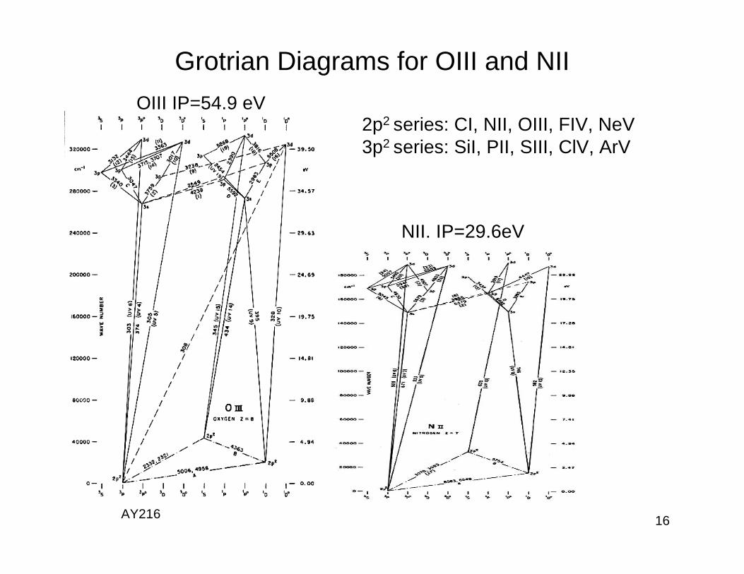
Grotrian Diagrams for OIII and NII

OIII IP=54.9 eV

NII. IP=29.6eV

2p2 series: CI, NII, OIII, FIV, NeV3p2 series: SiI, PII, SIII, ClV, ArV

AY216 17

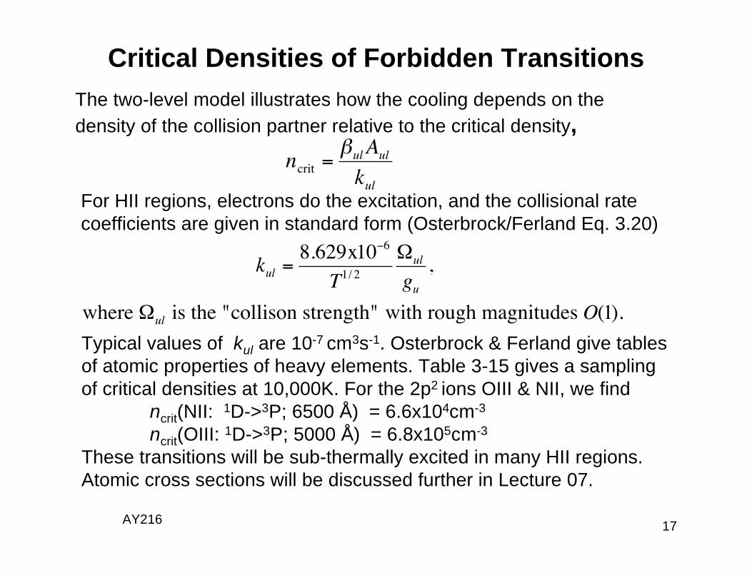
Critical Densities of Forbidden Transitions

The two-level model illustrates how the cooling depends on the

density of the collision partner relative to the critical density,

For HII regions, electrons do the excitation, and the collisional ratecoefficients are given in standard form (Osterbrock/Ferland Eq. 3.20)

ncrit = ul Aul

kul

kul =8.629x10 6

T1/ 2ul

gu,

where ul is the "collison strength" with rough magnitudes O(1).

Typical values of kul are 10-7 cm3s-1. Osterbrock & Ferland give tables of atomic properties of heavy elements. Table 3-15 gives a sampling of critical densities at 10,000K. For the 2p2 ions OIII & NII, we find

ncrit(NII: 1D->3P; 6500 Å) = 6.6x104cm-3

ncrit(OIII: 1D->3P; 5000 Å) = 6.8x105cm-3

These transitions will be sub-thermally excited in many HII regions.Atomic cross sections will be discussed further in Lecture 07.

AY216 18

Solution of the Temperature

Problem for HII Regions

Heating (minus recombination cooling)and line cooling plotted vs.T, theformer for stars with T* = 35,000 &50,000K (dashed lines). The solid linesare for line cooling with only a smallcontribution from free-free collisions.NII & OIII are the most Important.The unlabeled solid line is the total linecooling, and the solution where itcrosses a dashed line is near8,000K

Figure 3.3 of Osterbrock (1988). In the newedition of Osterbrock& Ferland the figure isslightly different due to revised abundancesand atomic parameters

AY216 19

Diagnostics of HII Regions

1. Measuring Temperature: The mere occurrence of optical forbidden lines suggests values of order 104 K.NB: E = (12,400 / ) and 1eV corresponds to 11,605 K.

More precisely, observing transitions of the same ion from different upper levels measures T, e.g., using the ratio of intensities of the 5007/4959 and 4363 lines of OIII.

The ratio changes from 2000 too 400 as T varies from 6,000 to 20,000 K

1S0 ------------------------

4363

1D2 -----------------------

4959, 5007

3PJ ------------------------

AY216 20

Diagnostics of HII Regions (cont’d)

2. Measuring Electron Density.

The critical densities vary from transitionto transition because A-values and ratecoefficients do, e.g., in the case ofdoublets leading to the ground state thevariation arises from statistical weights.

SII has strong red lines that arise fromthe first excited fine-structure doublet. Thecritical densities are ~ 104 cm s-1.

At low densities, the intensities aredetermined by the collision strengths,at high densities by the A-values.The net effect is a line-intensity ratiothat varies significantly with density.

2D5/2 ------------------------2D3/2 -----------------------

6731

67164S1/2 ------------------------

SII red lines

AY216 21

Combined Diagnostics:OIII Optical and Far Infrared Lines

Applied to Planetary Nebulae

Osterbrock (1988), Fig. 5.6

log ne

T

AY216 22

Summary

We have discussed the processes that produce HII regionsaround young, massive stars and that generate diagnosticemission lines that can be used to measure T and ne.

The forbidden lines of heavy atoms & ions are excited byelectronic collisions (in contrast to the recombination lines)so that, even in this simplest example of a photoionizednebulae, collisional phenomena play a role in so-calledphotoionization equilibrium.

Similar methods apply to the study of planetary nebulaeand quasar clouds, although additional processes haveto be considered, e.g., extreme FUV and X-ray ionization.

Many things are missing from this discussion, e.g., dynamiceffects, especially the fact that massive stars have powerfuloutflows, as well as the role of dust. For further details, seethe book by Ferland & Osterbrock.