lec03, speech i, v1.12.ppt -...

Multimedia SystemsMultimedia Systems

Speech ISpeech I

Course PresentationCourse Presentation

Mahdi Amiri

February 2014

Sharif University of Technology

SoundSound

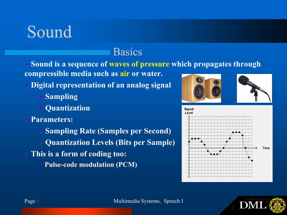
Sound is a sequence of waves of pressure which propagates through

compressible media such as air or water.

Digital representation of an analog signal

Sampling

Quantization

BasicsBasics

Page 1 Multimedia Systems, Speech I

Quantization

Parameters:

Sampling Rate (Samples per Second)

Quantization Levels (Bits per Sample)

This is a form of coding too:

Pulse-code modulation (PCM)

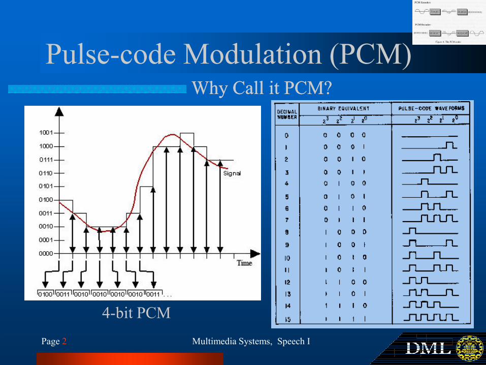
Pulse-code Modulation (PCM)Why Call it PCM?Why Call it PCM?


4-bit PCM

Audio: Sampling & Quantization

How to choose proper…

Sampling Rate

8 Khz ?

Quantization Level

8 bit/sample ?

Bit per Second (bit/s or bps)Bit per Second (bit/s or bps)


8 bit/sample ?

Bit per Second for 8000 Hz 8 bit PCM

64 kbit/s

• Low Sampling rate: Aliasing, Low quality in

reconstruction

• High Sampling rate: Data Redundancy, High

storage, High processing power consumption

• Low Quantization Levels: Large Q. noise, low SNR.

• High Quantization levels: More bits required, High

storage, High processing power consumption

Audio, Sampling

Human Hearing Frequency Range

20 Hz to 20 kHz

Most people will find that their hearing is most

sensitive around 1-4 kHz and that it is less sensitive at

Sampling RateSampling Rate


sensitive around 1-4 kHz and that it is less sensitive at

high and low frequencies.

Play with “Audacity”

tone generator to test

your hearing

audacity.sourceforge.net

Audio, SamplingTest your own hearing rangeTest your own hearing range


1 KHz

200 Hz100 Hz10 Hz

12 KHz 14 KHz 15 KHz 16 KHz 18 KHz

20 Hz

2 KHz

30 Hz 40 Hz

4 KHz

500 Hz50 Hz 75 Hz

8 KHz

3 Sec. tones

with

different

frequencies.

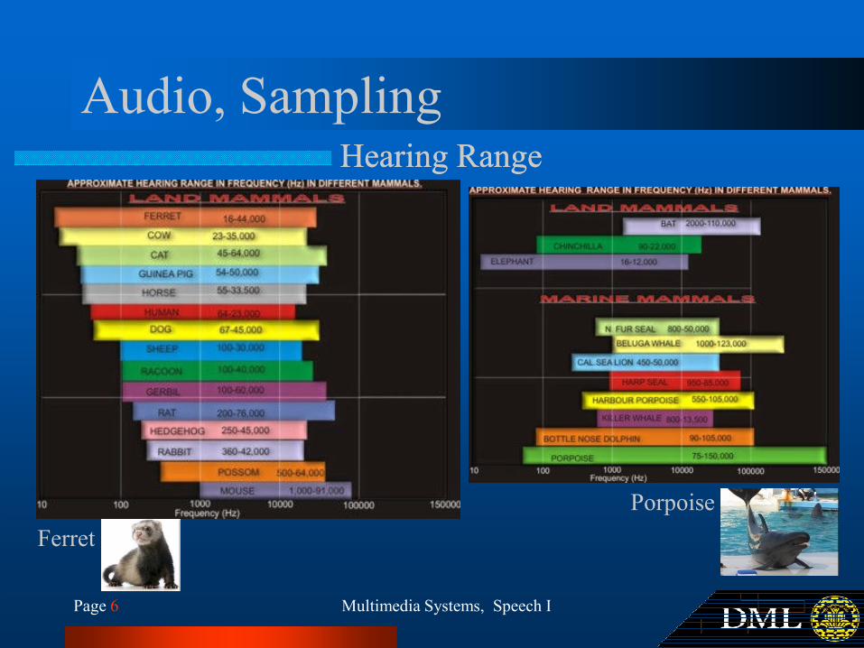
Audio, SamplingHearing RangeHearing Range


Ferret

Porpoise

Frequency AllocationsRadio Frequency BandsRadio Frequency Bands

9 KHz thr. 300 GHz

AM Radio

535 KHz thr. 1.6 MHz

FM Radio

88 MHz thr. 108 MHz

Also see "Communications Regulatory

Authority of The I.R of Iran"

www.cra.ir


United States radio spectrum frequency allocations chart as of 2011.

88 MHz thr. 108 MHz

TV

Various bands from

54 MHz thr. 700 MHz

GSM (Global System for

Mobile Communications)

Mostly 900 MHz and

1800 MHZ

ModulationAM, FM, PMAM, FM, PM

Signal (or message):

Amplitude Modulation (AM) conveys information over

a carrier wave (the transmitted signal) by varying the

amplitude (strength) of the carrier in relation to the

information being sent ( carrier's frequency remains

constant).

Carrier:


A signal may be carried by an AM or FM radio wave.

Phase Modulation (PM) represents

information as variations in the instantaneous

phase of a carrier wave.

PM Example

Frequency Modulation (FM) works by varying

carrier's instantaneous frequency.

PM

and

Audio, Sampling

Human Vocal Range

Normal: 80 Hz to 1100 Hz

Guinness Book of Records

Female: Georgia Brown

Sampling RateSampling Rate


Female: Georgia Brown

Eight octaves

G2 (97.9989 Hz) thr. G10 (25087.7150 Hz)

Male: Tim Storms

Ten octaves (0.7973 Hz thr. 807.3 Hz)

www.guinnessworldrecords.com/world-records/1000/greatest-vocal-range-female

www.guinnessworldrecords.com/world-records/3000/greatest-vocal-range-male

Octave: In music, an octave is the interval between one musical pitch and another with half or double its frequency.

Play and see! Low

freq. voice of Tim

Storms, as you may

can’t hear it.

Audio, Sampling

8,000 Hz - Telephone, adequate for human speech.

11,025 Hz – lower quality PCM (one quarter the sampling rate of audio CDs).

22,050 Hz – Radio.

32,000 Hz - miniDV digital video camcorder, DAT (LP mode).

44,100 Hz - Audio CD, also most commonly used with MPEG-1 audio (VCD, SVCD,

MP3) (Originally chosen by Sony, 1979).

Common Sampling RatesCommon Sampling Rates


MP3) (Originally chosen by Sony, 1979).

48,000 Hz - Digital sound used for miniDV, digital TV, DVD, DAT, films and

professional audio.

96,000 or 192,000 Hz - DVD-Audio, some LPCM DVD tracks, BD-ROM (Blu-ray

Disc) audio tracks, and HD-DVD (High-Definition DVD) audio tracks.

2.8224 MHz - Super Audio CD (SACD), 1-bit sigma-delta modulation process known

as Direct Stream Digital (DSD), co-developed by Sony and Philips.

5.6448 MHz - Double-Rate DSD, 1-bit Direct Stream Digital at 2x the rate of the

SACD. Used in some professional DSD recorders (128 * 44100 Hz).

DXD - 24-bit sampled at 352.8 kHz, suited for editing, eq. with 8.4672 MHz 1-bit DSD

Pulse-code Modulation (PCM)

The trademark name used by Sony and Philips.

Uses pulse-density modulation encoding

Direct Stream DigitalDirect Stream Digital


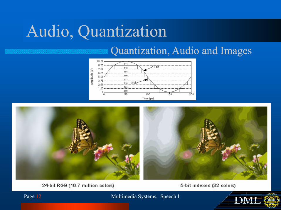
Audio, QuantizationQuantization, Audio and ImagesQuantization, Audio and Images


Audio, Quantization

Simple and popular

Midtread

Odd number of

reconstruction levels (N)

(quantizing levels)

Uniform Uniform QuantizerQuantizer, , MidtreadMidtread


(quantizing levels)

Here N = 9

Audio, Quantization

Simple and popular

Midrise

Even number of

reconstruction levels

Here N = 8

Uniform Uniform QuantizerQuantizer, Midrise, Midrise


Here N = 8

Quantization error for bounded input

Audio, Quantization

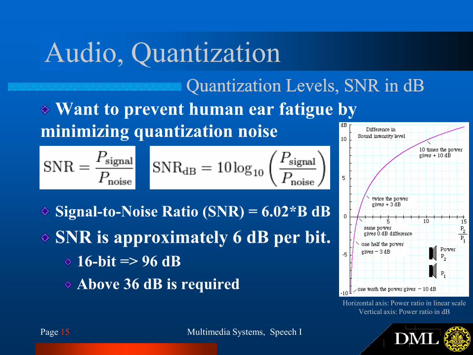
Want to prevent human ear fatigue by

minimizing quantization noise

Quantization Levels, SNR in dBQuantization Levels, SNR in dB


Signal-to-Noise Ratio (SNR) = 6.02*B dB

SNR is approximately 6 dB per bit.

16-bit => 96 dB

Above 36 dB is requiredHorizontal axis: Power ratio in linear scale

Vertical axis: Power ratio in dB

Audio, Quantization

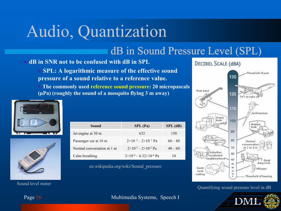
dB in SNR not to be confused with dB in SPL

SPL: A logarithmic measure of the effective sound

pressure of a sound relative to a reference value.

The commonly used reference sound pressure: 20 micropascals

(µPa) (roughly the sound of a mosquito flying 3 m away)

dB in Sound Pressure Level (SPL)dB in Sound Pressure Level (SPL)


en.wikipedia.org/wiki/Sound_pressure

Quantifying sound pressure level in dB

Sound SPL (Pa) SPL (dB)

Jet engine at 30 m 632 150

Passenger car at 10 m 2×10−2 – 2×10−1 Pa 60 – 80

Normal conversation at 1 m 2×10-3 – 2×10-2 Pa 40 – 60

Calm breathing 2×10-4 – 6.32×10-4 Pa 10

Sound level meter

Audio, QuantizationdBAdBA in Sound Pressure Level (SPL)in Sound Pressure Level (SPL)

The human ear responds more to

frequencies between 500 Hz and 8 kHz

and is less sensitive to very low-pitch or

high-pitch noises. The frequency

weightings used in sound level meters are

often related to the response of the human


often related to the response of the human

ear, to ensure that the meter is measuring

pretty much what you actually hear.

A-Weighted frequency response �

dBZ: means no weighting at all

Audio, QuantizationVSLMVSLM

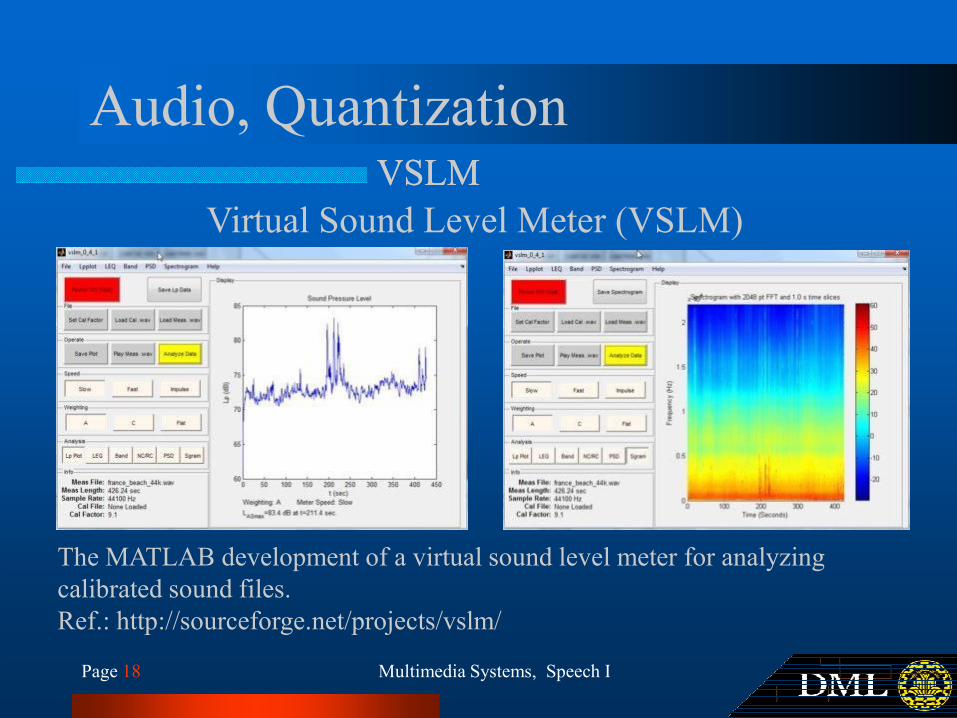
Virtual Sound Level Meter (VSLM)


The MATLAB development of a virtual sound level meter for analyzing

calibrated sound files.

Ref.: http://sourceforge.net/projects/vslm/

Audio, QuantizationQuantization Levels, SNR in dBQuantization Levels, SNR in dB

0 0.5 1 1.5 2 2.5 3 3.5

x 104

-1

-0.8

-0.6

-0.4

-0.2

0

0.2

0.4

0.6

0.8

Click to play

original sound

Text: A lathe is a big tool. Grab every dish of sugar.


Sample output of SpeechNoise_T03.m (Play noisy speech with different SNR values)

-10 dB 0 dB

10 dB 20 dB

30 dB 40 dB

50 dB 60 dB

70 dB 80 dB

90 dB

Audio, Quantization6 dB per bit rule of thump6 dB per bit rule of thump

[ ] [ ] [ ]ˆe x xn n n= −

[ ]m mX x n X− < <

Average power of a process or signal:

( ) ( )2 2

x xx p x dxµ σ+∞

−∞− =∫

xµ ( )p x : Probability density function: Mean

( ) ( )2 210logSNR B σ σ=

: Variance

0µ = ( ) 1p e =


[ ]2 2e n∆ ∆− < ≤

[ ]m mX x n X− < <

[ ]Assumption: is uniform over ( , ]2 2

e n ∆ ∆−

The probability density function of e[n]

2

2

m

B

X∆ =

( ) ( )2 2

1010logdB x eSNR B σ σ=

( ) ( )22

22 22 2

22 2

1

12 2 3

me e B

Xe p e de e deσ µ

∆ ∆+ +

∆ ∆− −

∆= − = = =

∆ ×∫ ∫

( ) ( )( ) ( )

2 2 2

10

2 2

10 10

10log 2 3

20log 2 10log 3

B

dB x m

x m

SNR B X

B X

σ

σ

=

= +

( ) ( )2 2

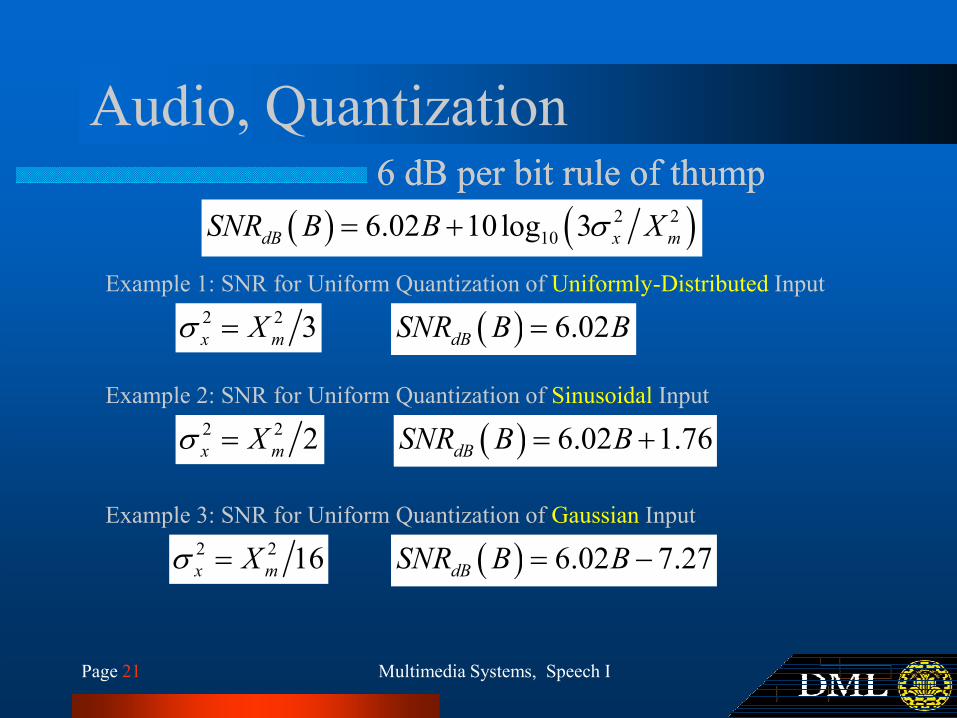
106.02 10log 3dB x mSNR B B Xσ= +

0eµ = ( ) 1

p e =∆

Audio, Quantization6 dB per bit rule of thump6 dB per bit rule of thump

Example 1: SNR for Uniform Quantization of Uniformly-Distributed Input

( ) ( )2 2

106.02 10log 3dB x mSNR B B Xσ= +

2 2 3x mXσ = ( ) 6.02dBSNR B B=


Example 2: SNR for Uniform Quantization of Sinusoidal Input

2 2 2x mXσ = ( ) 6.02 1.76dBSNR B B= +

Example 3: SNR for Uniform Quantization of Gaussian Input

2 2 16x mXσ = ( ) 6.02 7.27dBSNR B B= −

Audio, Bit-rate

The average person cannot tell the difference between a bitrate above 192

kbit/s and the original CD/WAV.

Even if your headphones seal really well around your ears, they will

probably only give you about 20 to 25 dB insulation from the external sound

Good to KnowGood to Know


20 ~ 25 dB insulation

Noise level for 192 kbps audio is under -125 dB and certainly inaudibleMeaning of this dB: Noise power after coding and decoding over original signal power in logarithmic scale.

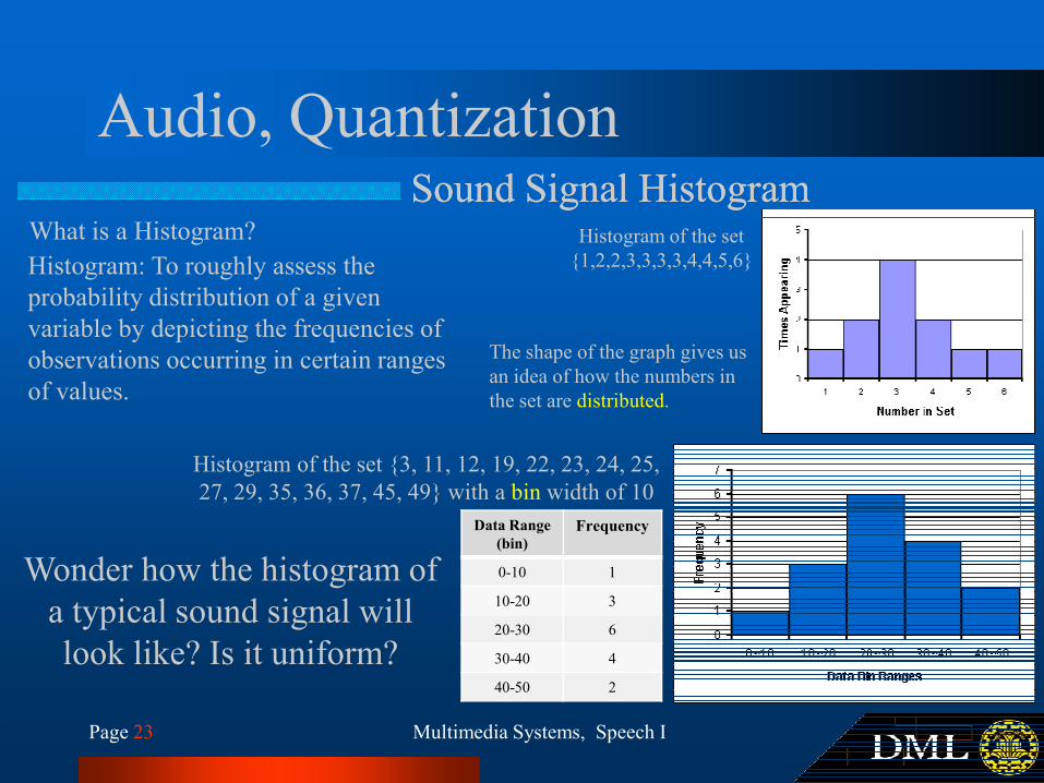
Audio, QuantizationSound Signal HistogramSound Signal Histogram

Histogram of the set

{1,2,2,3,3,3,3,4,4,5,6}

What is a Histogram?

Histogram: To roughly assess the

probability distribution of a given

variable by depicting the frequencies of

observations occurring in certain ranges

of values.

The shape of the graph gives us

an idea of how the numbers in

the set are distributed.


of values. the set are distributed.

Wonder how the histogram of

a typical sound signal will

look like? Is it uniform?

Histogram of the set {3, 11, 12, 19, 22, 23, 24, 25,

27, 29, 35, 36, 37, 45, 49} with a bin width of 10

Data Range

(bin)

Frequency

0-10 1

10-20 3

20-30 6

30-40 4

40-50 2

Audio, QuantizationTypical Speech Signal WaveformTypical Speech Signal Waveform

0 0.5 1 1.5 2 2.5 3 3.5

x 104

-1

0

1Original sound

6200-7200

See SpeechHistT01.m


100 200 300 400 500 600 700 800 900 1000-1

0

16200-7200

10 20 30 40 50 60 70 80 90 100-1

0

16450-6550

Audio, QuantizationTypical Speech Signal HistogramTypical Speech Signal Histogram

0.5

1

1.5

2

x 104

8-bins

0.5

1

1.5

2

x 104

16-bins

figure;

hist( x, 256 );

axis([-1 1 -inf inf])

-1 -0.8 -0.6 -0.4 -0.2 0 0.2 0.4 0.6 0.8 10

2000

4000

6000

8000

10000


256-bins

-1 -0.8 -0.6 -0.4 -0.2 0 0.2 0.4 0.6 0.8 10

0.5

-1 -0.8 -0.6 -0.4 -0.2 0 0.2 0.4 0.6 0.8 10

0.5

-1 -0.8 -0.6 -0.4 -0.2 0 0.2 0.4 0.6 0.8 10

2000

4000

6000

8000

10000

12000

14000

64-bins

Audio, QuantizationUniform Uniform QuantizerQuantizer, , MidtreadMidtread

50 100 150 200 250 300 350 400 450 500-1

-0.5

0

0.5

1Original sound

Quantized signal

See SpeechQuantizationT02.m

Original (17700:18200)

aQ_Partition = [-0.8750 -0.6250 -0.3750 -0.1250 0.1250 0.3750 0.6250];

aQ_Codebook = [-1.0000 -0.7500 -0.5000 -0.2500 0 0.2500 0.5000 0.7500];


50 100 150 200 250 300 350 400 450 500-1

-0.5

0

0.5

1Quantized signal

50 100 150 200 250 300 350 400 450 500-1

-0.5

0

0.5

1

Original signal

Quantized signal

3-bit Quantized

Audio, QuantizationUniform Uniform QuantizerQuantizer, Midrise, Midrise

50 100 150 200 250 300 350 400 450 500-1

-0.5

0

0.5

1Original sound

Quantized signal


Original (17700:18200)

aQ_Partition = [-0.7500 -0.5000 -0.2500 0 0.2500 0.5000 0.7500];

aQ_Codebook = [-0.8750 -0.6250 -0.3750 -0.1250 0.1250 0.3750 0.6250 0.8750];


50 100 150 200 250 300 350 400 450 500-1

-0.5

0

0.5

1Quantized signal

50 100 150 200 250 300 350 400 450 500-1

-0.5

0

0.5

1

Original signal

Quantized signal

3-bit Quantized

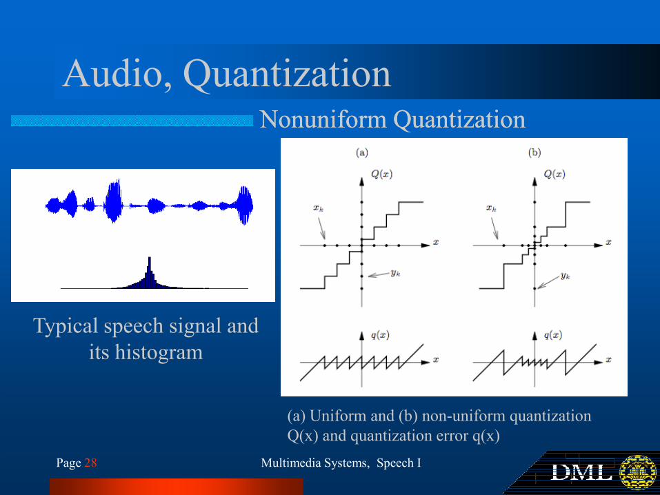
Audio, QuantizationNonuniformNonuniform QuantizationQuantization


(a) Uniform and (b) non-uniform quantization

Q(x) and quantization error q(x)

Typical speech signal and

its histogram

Audio, QuantizationUniform Uniform QuantizerQuantizer, , MidtreadMidtread

50 100 150 200 250 300 350 400 450 500-1

-0.5

0

0.5

1Original sound

Quantized signal


Original (17700:18200)

aQ_Partition = [-0.8750 -0.6250 -0.3750 -0.1250 0.1250 0.3750 0.6250];

aQ_Codebook = [-1.0000 -0.7500 -0.5000 -0.2500 0 0.2500 0.5000 0.7500];

* Deliberately repeated slide


50 100 150 200 250 300 350 400 450 500-1

-0.5

0

0.5

1Quantized signal

50 100 150 200 250 300 350 400 450 500-1

-0.5

0

0.5

1

Original signal

Quantized signal

3-bit Quantized

Audio, QuantizationNonNon--Uniform Uniform QuantizerQuantizer


50 100 150 200 250 300 350 400 450 500-1

-0.5

0

0.5

1Original sound

Quantized signal

Original (17700:18200)

aQ_Partition = [-0.5 -0.25 -0.1 -0.05 0.05 0.1 0.25];

aQ_Codebook = [-0.6 -0.32 -0.17 -0.075 0 0.075 0.17 0.32];

Play and compare quantized speech in MATLAB


50 100 150 200 250 300 350 400 450 500-1

-0.5

0

0.5

1Quantized signal

50 100 150 200 250 300 350 400 450 500-1

-0.5

0

0.5

1

Original signal

Quantized signal

3-bit Quantized

Audio, QuantizationQuantization Levels, SNR in dBQuantization Levels, SNR in dB

0 0.5 1 1.5 2 2.5 3 3.5

x 104

-1

-0.8

-0.6

-0.4

-0.2

0

0.2

0.4

0.6

0.8

Click to play

original sound

Text: A lathe is a big tool. Grab every dish of sugar.

NonUniQ_3_bit_snr_24.2493_dB.auUniQ_3_bit_MidTread_snr_14.8078_dB.auUniQ_3_bit_MidRise_snr_2.9701_dB.au


Sample output of SpeechQuantizationT01.m thr. SpeechQuantizationT03.m

(Uniform and Nonuniform Speech Quantization)

UniQ_4_bit_MidTread_snr_25.0756_dB.auUniQ_4_bit_MidRise_snr_15.8282_dB.au

UniQ_5_bit_MidTread_snr_36.167_dB.auUniQ_5_bit_MidRise_snr_28.4824_dB.au

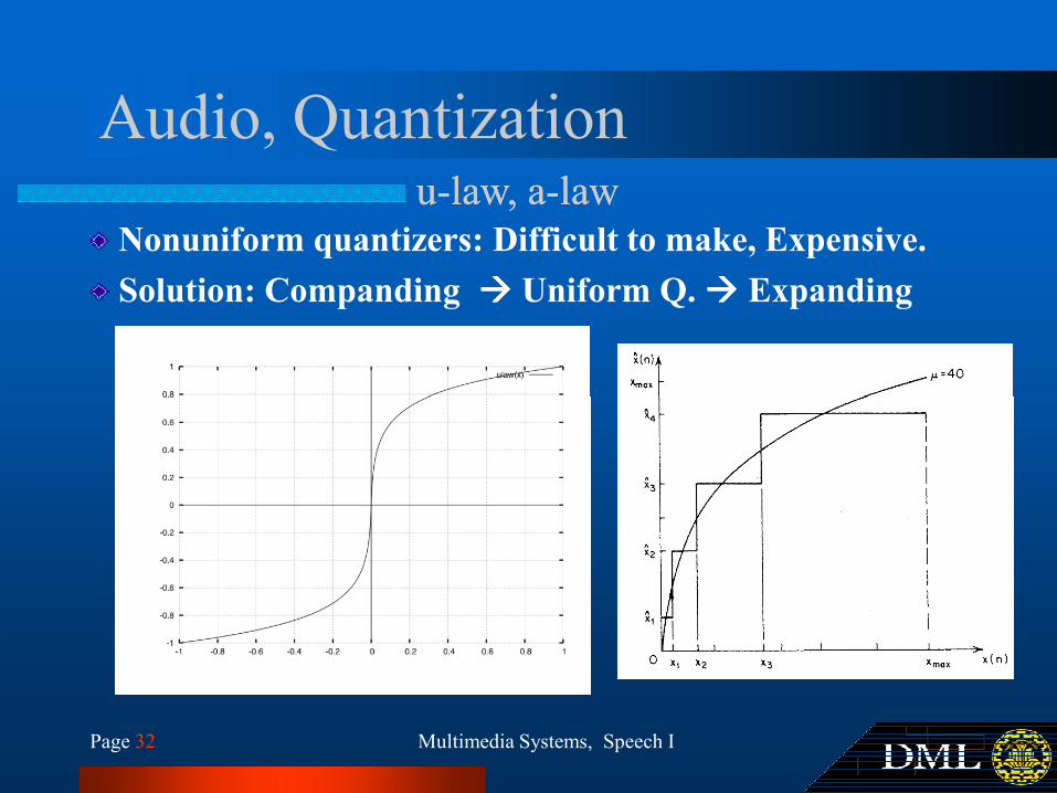
Audio, Quantization

Nonuniform quantizers: Difficult to make, Expensive.

Solution: Companding �� Uniform Q. �� Expanding

uu--law, alaw, a--lawlaw


Audio, Quantizationuu--law, alaw, a--lawlaw


Audio, Quantizationuu--law, alaw, a--lawlaw


u-law

North America and Japan

a-law

Europe

HomeworkSpeech QuantizationSpeech Quantization

Compander

Uniform

Original Sound

Quantization

Companding

parameter (µ)


Uniform

Quantizer

Dequantizer

Expander

SNR Calculation

µ-law encoded

sound

Quantization

bit No.

Plot and Play

MATLAB code or GUI implementation (Take a look at Speech noise test MATLAB codes to

have sample input signal and to find out more about how to plot and play the sounds.

+

-

Make a plot and show how SNR changes with different values for Mu and B.

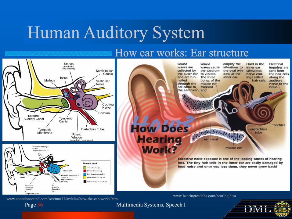
Human Auditory SystemHow ear works: Ear structureHow ear works: Ear structure


www.soundonsound.com/sos/mar11/articles/how-the-ear-works.htmwww.hearingtestlabs.com/hearing.htm

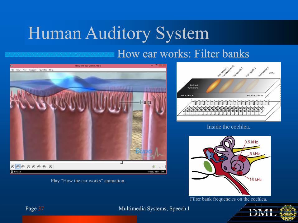
Human Auditory SystemHow ear works: Filter banksHow ear works: Filter banks


Play “How the ear works” animation.

Filter bank frequencies on the cochlea.

Inside the cochlea.

Audio, SamplingAliasing due to low samplingAliasing due to low sampling

Supplementary


Properly sampled image of brick

wall.

Spatial aliasing in the

form of a Moiré

pattern.

Two different sinusoids that

fit the same set of samples.

Thank You

Multimedia SystemsMultimedia Systems

Speech ISpeech I


Thank You

1. http://ce.sharif.edu/~m_amiri/

2. http://www.dml.ir/

FIND OUT MORE AT...

Next Session: Speech IINext Session: Speech II

lec03, speech i, v1.12.ppt -...

Documents