lecture 05 gerard medioni - tensor voting: fundamentals and recent progress
TRANSCRIPT

Tensor Voting in 2 to N Dimensions:
Fundamental Elements and Applications
Gérard Medioni
Institute for Robotics and Intelligent Systems
Viterbi School of Engineering
University of Southern California

Motivation
Computer vision problems are often inverse
■ Ill-posed
■ Computationally expensive
■ Severely corrupted by noise
Many of them can be posed as perceptual
grouping of primitives
■ Solutions form perceptually salient non-accidental
structures (e.g. surfaces in stereo)
■ Only input/output modules need to be adjusted in
most cases

Motivation
Develop an approach that is:
■General
■Data-driven
Axiom: the whole is greater than the sum of
the parts
Employ Gestalt principles of proximity and
good continuation to infer salient structures
from data

Representation
21/2-D sketch
■viewer-centered
input partition
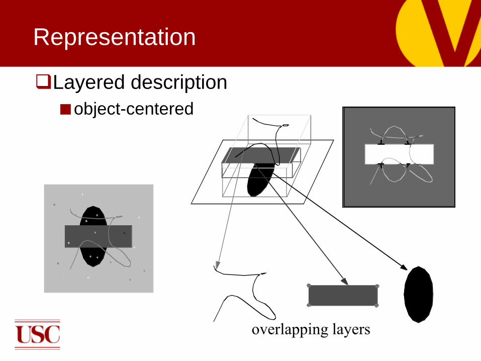
Representation
Layered description
■object-centered
overlapping layers

21/2-D sketch: stereo
Holes in middle and bottom surfaces
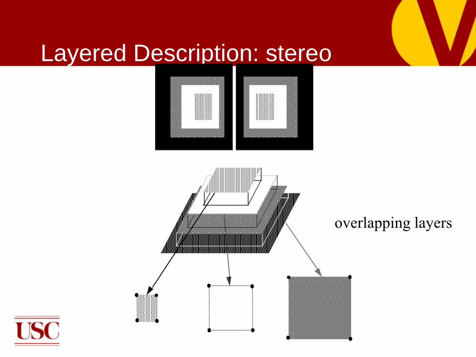
Layered Description: stereo
overlapping layers

21/2-D sketch: motion
Segmentation into regions

Layered Description: motion
overlapping layers

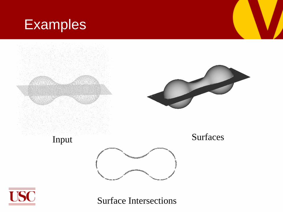
Examples

Desired Properties
Local, data-driven descriptions
■ More general, model-free solutions
■ Local changes affect descriptions locally
■ Global optimization often requires simplifying assumptions (NP-complete problems)
Ability to represent all structure types and their
interactions
Ability to process large amounts of data
Robustness to noise
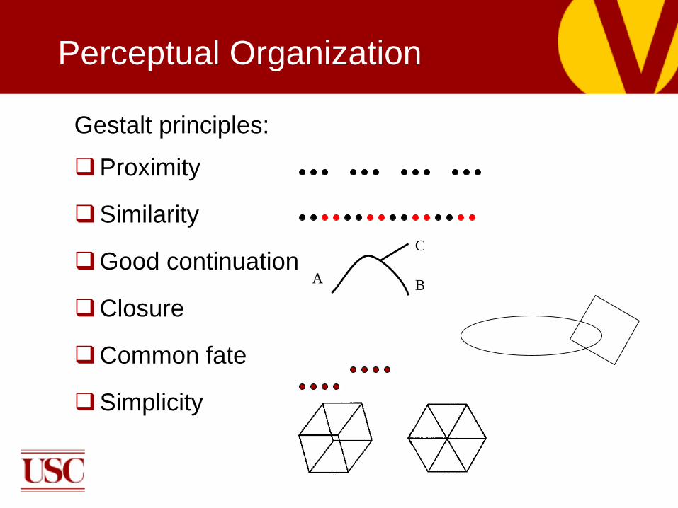
Perceptual Organization
Gestalt principles:
Proximity
Similarity
Good continuation
Closure
Common fate
Simplicity
A B
C

The Smoothness Constraint
Matter is
cohesive Smoothness
Difficult to implement, as true “almost everywhere” only

Related Work
Regularization
Relaxation Labeling
Robust Methods (RANSAC)
Level Set Methods
Clustering (Graph Cuts)
Perceptual Organization (Shashua and Ullman,
Grossberg and Mingolla, Heitger and von der Heydt, Lowe,
Williams)

Differences with our Approach
Infer all structure types simultaneously and
allow interaction between them
Can begin with oriented or unoriented
inputs (or both)
No prior model
No objective/cost function
Solution emerges from data

The Tensor Voting Framework
Data Representation: Tensors
Constraint Representation: Voting fields
■enforce smoothness
Communication: Voting
■non-iterative
■no initialization required
[Medioni, Lee, Tang 2000]

Our Approach in a Nutshell
Each input site propagates its information in a neighborhood
Each site collects the information castthere
Salient features correspond to local extrema of saliency
Properties of Tensor Voting
Non-Iterative (or few iterations)
Can extract all features simultaneously
One parameter (scale)
Non-critical thresholds
Efficient

Overview
Tensor Voting in 2-D
Tensor Voting in 3-D
Applications to Computer Vision
■Figure Completion
■Stereo
■Motion
Tensor Voting in N-D
Probabilistic Tensor Voting
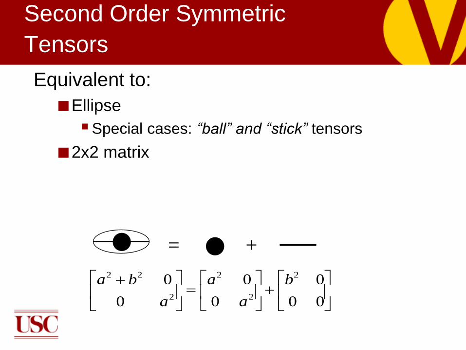
Second Order Symmetric
Tensors
Equivalent to:
■Ellipse
Special cases: “ball” and “stick” tensors
■2x2 matrix
+=
00
0
0
0
0
0 2
2
2
2
22 b
a
a
a
ba

Properties captured by second order
symmetric Tensor
■shape: orientation certainty
■size: feature saliency
Second Order Symmetric
Tensors

Representation with Tensors
Input Second Order Tensor Eigenvalues Quadratic Form
1=1 2=0
2
2
yyx
yxx
nnn
nnn
1=2=1
10
01

Design of the Voting Field
?

Notes on the design
A circle minimizes the total curvature, up to 45o
ASSIGNMENT: Prove it is NOT true beyond
45o
Hint1:
Hint 2:

Saliency Decay Function
Votes attenuate with length of smoothest path
Straight continuation is favored over curved
l
ls
sin2
sin
)(2
22
),(
cs
esS
x
y
P
s
2
l
Csin2
l
O

Notes on the Decay function
Choice of decay is not unique
Any bell-shape will do
Exp is convenient
Assignment: how would you select the
constant c which controls decay with
curvature?

Fundamental Stick Voting Field

Fundamental Stick Voting Field
All other fields in any N-D space are generated
from the Fundamental Stick Field:
■Ball Field in 2-D
■Stick, Plate and Ball Field in 3-D
■Stick, …, Ball Field in N-D
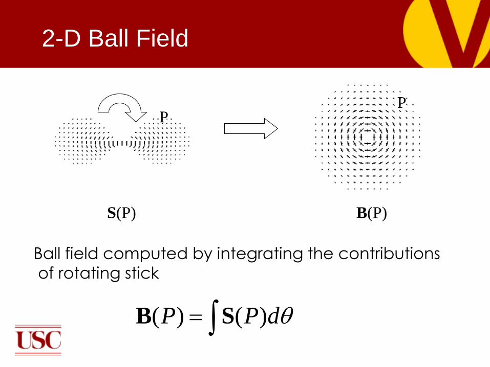
2-D Ball Field
Ball field computed by integrating the contributions
of rotating stick
dPP )()( SB
S(P) B(P)
PP

2-D Voting Fields
votes with
votes with
votes with +
Each input site propagates its information in a neighborhood

Voting
Voting from a ball tensor is isotropic
■Function of distance only
The stick voting field is aligned with the
orientation of the stick tensor
O
P

Mixed Voting
The framework allows voting with mixed input,
i.e. both oriented and isotropic tokens.
Assignment:
What should be the relative weight of a
oriented vs. isotropic token

Vote Accumulation
Each site accumulates second order votes by
tensor addition:
Results of accumulation are usually generic tensors

Illustration (ball vote)

Illustration (stick vote)
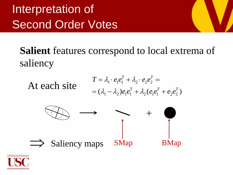
Interpretation of
Second Order Votes
Salient features correspond to local extrema of
saliency
At each site
+
Saliency maps SMap BMap
)()( 221121121
222111
TTT
TT
eeeeee
eeeeT

Vote Analysis
λ1- λ2» 0: stick saliency is larger than ball
saliency. Likely on curve.
λ1≈λ2 » 0: ball saliency larger than stick
saliency. Likely junction (or region).
λ1≈λ2 ≈ 0: Low saliency. Outlier.
)()( 221121121
222111
TTT
TT
eeeeee
eeeeT
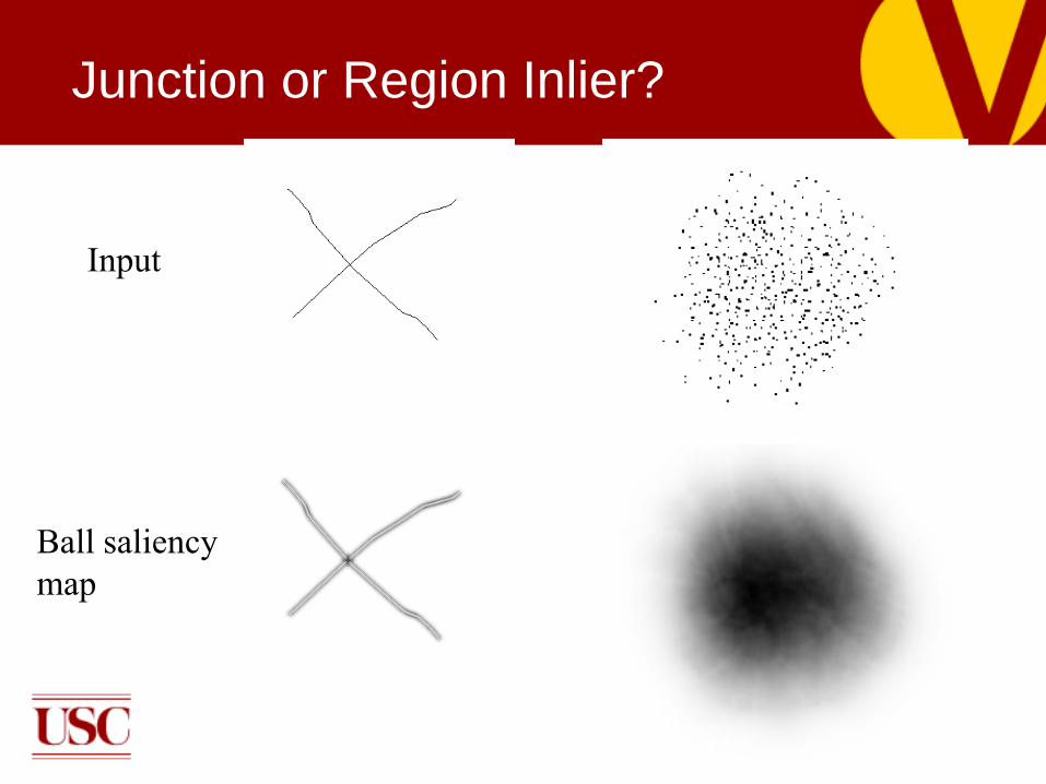
Junction or Region Inlier?
Input
Ball saliency
map

Results in 2-D
Scale of Voting
The Scale of Voting is the single critical
parameter in the framework
Essentially defines size of voting
neighborhood
■Gaussian decay has infinite extend, but it is
cropped to where votes remain meaningful (e.g.
1% of voter saliency)
Scale of Voting
The Scale is a measure of the degree of smoothness
Smaller scales correspond to small voting neighborhoods, fewer votes■ Preserve details
■ More susceptible to outlier corruption
Larger scales correspond to large voting neighborhoods, more votes■ Bridge gaps
■ Smooth perturbations
■ Robust to noise

Sensitivity to Scale
A
B
Input
= 50
= 500
= 5000
Curve saliency as a function of scale
Blue: curve saliency at A
Red: curve saliency at B
Input: 166 un-oriented inliers, 300 outliers
Dimensions: 960x720
Scale ∈ [50, 5000]
Voting neighborhood ∈ [12, 114]

Sensitivity to Scale
Circle with radius 100 (unoriented tokens)
As more information is accumulated,
the tokens better approximate the circle
Scale Average angular error (degrees)
50 1.01453
100 1.14193
200 1.11666
300 1.04043
400 0.974826
500 0.915529
750 0.813692
1000 0.742419
2000 0.611834
3000 0.550823
4000 0.510098
5000 0.480286

Sensitivity to Scale
Square 20x20 (unoriented tokens)
As scale increases to unreasonable levels (>1000)
corners get rounded
Junctions are detected and excluded
Scale Average angular error (degrees)
50 1.11601e-007
100 0.138981
200 0.381272
300 0.548581
400 0.646754
500 0.722238
750 0.8893
1000 1.0408
2000 1.75827
3000 2.3231
4000 2.7244
5000 2.98635

Illustration of Tensor Voting

Example in 2-D
Input
Stick saliency
Output
Ball saliency

Summary
Feature Extraction
Saliency tensor field(dense)
Encode
Input tokens(sparse)
dots
Tensor Voting
Tensor tokens(sparse)
tensors
Tensor tokens(refined)
Tensor Voting
tensors

Boundaries?
Input
Saliency
No clear way to detect the endpoints of the curve
with second order Tensor Voting

Need for First Order Information
Second order Tensor Voting can infer curves and junctions
Second order tensors at A, B, D and E are very similar, but A and B are very different from D and E
Key property of endpoints: all neighbors are on same side

Polarity Vectors
Representation augmented with Polarity
Vectors
Vectors are first order tensors
Sensitive to direction from which votes are
received
Exploit property of boundaries to have all
their neighbors on the same side of the half-
space

First Order Voting
Votes are cast along the
tangent of the smoothest
path
Vector votes instead of
tensor votes
Accumulated by vector
addition
Boundaries have all their
neighbors on the same
side of the half-space
x
y
P
s
C
O
l
Second order vote
First order vote

First Order Voting Fields
Magnitude is the same as in the second order
case
First-order Ball field can be derived from the
first-order Stick Field after integration
)(2
22
),(
cs
esS

Endpoint Inference
Input
Saliency
Polarity

Illustration of First Order Voting
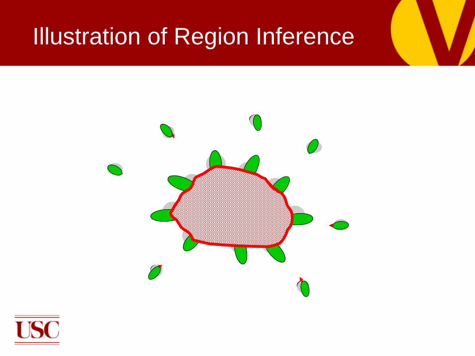
Illustration of Region Inference
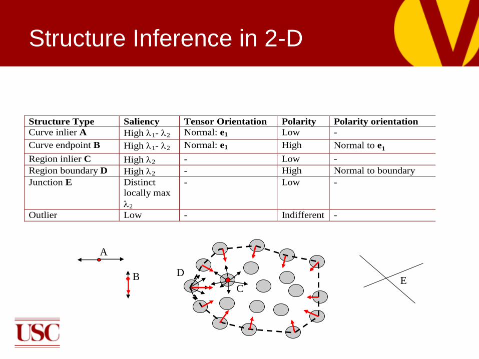
Structure Inference in 2-D
Structure Type Saliency Tensor Orientation Polarity Polarity orientation
Curve inlier A High 1- 2 Normal: e1 Low -
Curve endpoint B High 1- 2 Normal: e1 High Normal to e1
Region inlier C High 2 - Low -
Region boundary D High 2 - High Normal to boundary
Junction E Distinct
locally max
2
- Low -
Outlier Low - Indifferent -
A
B D
CE

Example in 2-D

Results
Gray: curve inliers
Black: curve endpoints
Squares: junctions
Input

Results
Input Curves and endpoints only Curves, endpoints
and regions
Overview
Tensor Voting in 2-D
Tensor Voting in 3-D
Applications to Computer Vision
■Figure Completion
■Stereo
■Motion
Tensor Voting in N-D
Probabilistic Tensor Voting

3-D Tensor Voting
Representation: 3-D Tensors
Constraints: 3-D Voting Fields
Data communication: Voting
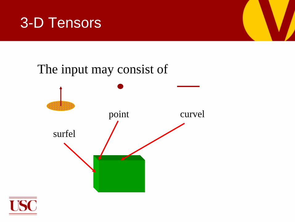
3-D Tensors
The input may consist of
point curvel
surfel

3-D Tensor Decomposition
ball
tensorplate
tensor
stick
tensor
3 eigenvalues
(max mid min )
3 eigenvectors
(emax emid emin )

3-D Second Order Tensors
Encode normal orientation in tensor
Surfel: 1 normal “stick” tensor
Curvel: 2 normals “plate” tensor
Point/junction: 3 normals “ball” tensor

Representation

3-D Tensor Analysis
Surface saliency: λ1- λ2 normal: e1
Curve saliency: λ2- λ3 normals: e1 and e2
Junction saliency: λ3
)())(()( 33221132211321121
333222111
TTTTTT
TTT
eeeeeeeeeeee
eeeeee
T
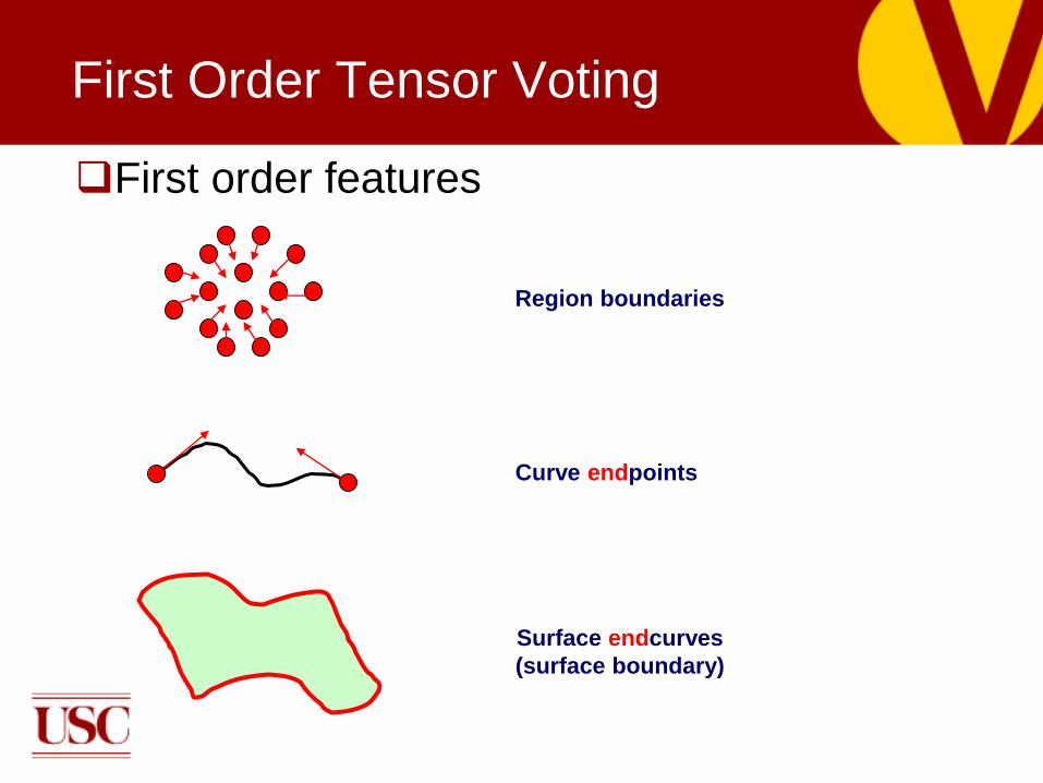
First Order Tensor Voting
First order features
Curve endpoints
Surface endcurves
(surface boundary)
Region boundaries

Interpretation of Resulting Tensors
Structure Type Saliency Tensor
Orientation
Polarity Polarity orientation
Surface inlier High 1- 2 Normal: e1 Low -
Surface boundary High 1- 2 Normal: e1 High Normal to e1 and
boundary
Curve inlier High 2- 3 Tangent: e3 Low -
Curve endpoint High 2- 3 Tangent: e3 High Parallel to e3
Volume inlier High 3 - Low -
Volume boundary High 3 - High Normal to bounding
surface
Junction Distinct
locally max 3
- Low -
Outlier Low - Indifferent -
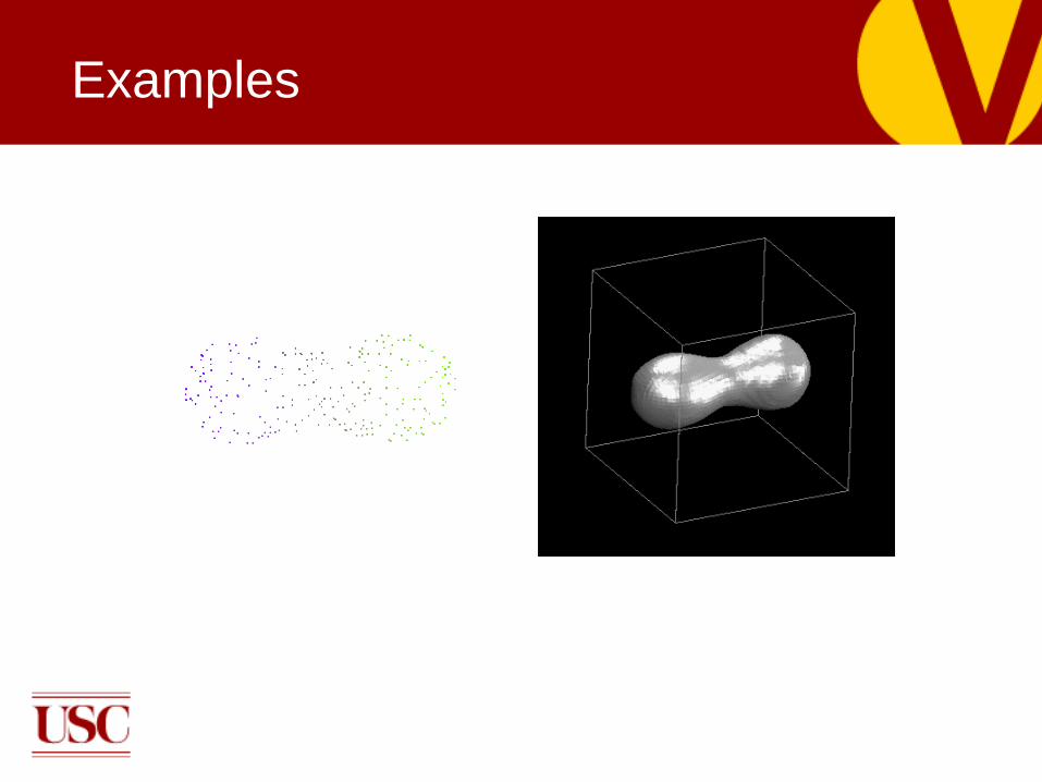
Examples

Examples
Examples
Input Surfaces
Surface Intersections

Examples
Input Volume Boundaries

Examples
Input Surfaces - Surface Boundaries – Surface Intersections
Curves – Endpoints - Junctions

Graceful Degradation with Noise
67% noise75% noise80% noise

Results in 3-D
Input (600k unoriented points) Input with 600k outliers
Output with 1.2M outliers Output with 2.4M outliers

Overview
Tensor Voting in 2-D
Tensor Voting in 3-D
Applications to Computer Vision
■Figure Completion
■Stereo
■Motion
Tensor Voting in N-D
Probabilistic Tensor Voting

Figure Completion
Amodal completion
Modal completion Layered interpretation

Motivation
Approach for modal and amodal completion
Automatic selection between them
Explanation of challenging visual stimuli
consistent with human visual system
[Mordohai and Medioni, POCV 2004]

Keypoint Detection
Input binary images
Infer junctions, curves, endpoints, regions
and boundaries
Look for completions supported by
endpoints, L and T-junctions
W, X and Y-junctions do not support
completion by themselves

Support for Figure Completion
Amodal:
■ Along the tangent of endpoints
■ Along the stem of T-junctions
Modal:
■ Orthogonal to endpoints
■ Along the bar of T-junctions
■ Along either edge of L-junctions

Results: Modal Completion
Input Curves and endpoints Curve saliency Output

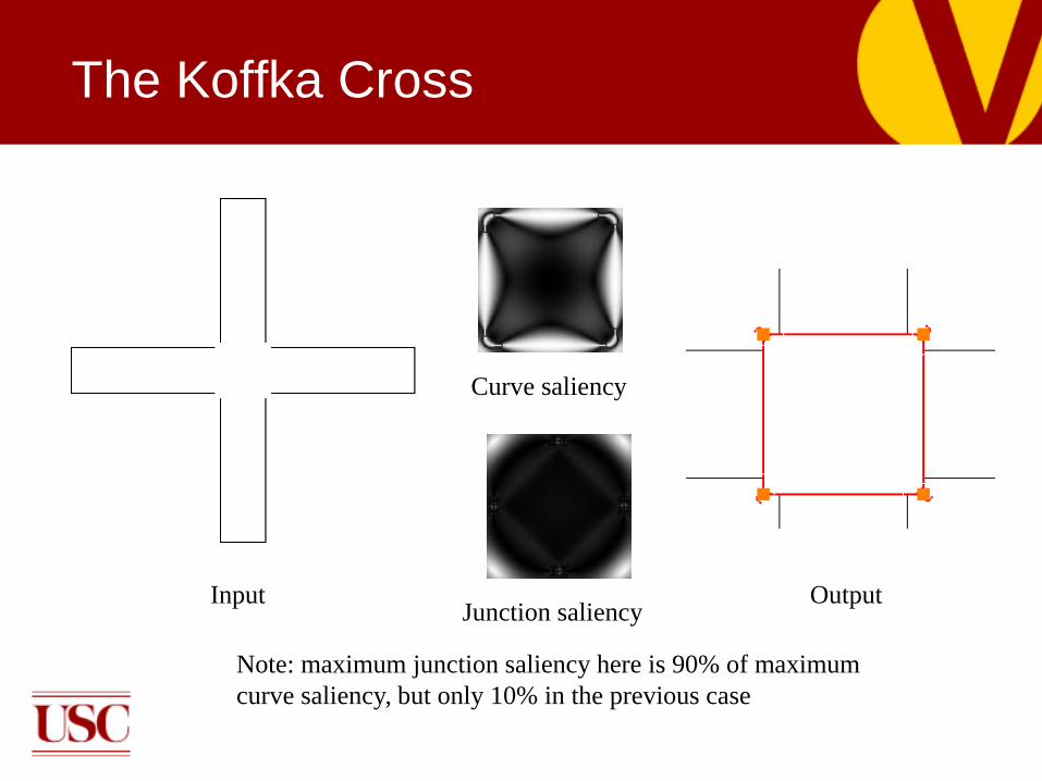
The Koffka Cross
Input
Curve saliency
OutputJunction saliency
The Koffka Cross
Input
Curve saliency
OutputJunction saliency
Note: maximum junction saliency here is 90% of maximum
curve saliency, but only 10% in the previous case

Koffka Cross: Amodal
Completion
Curve saliency
OutputJunction saliency
Amodal completion
(occluded)

The Poggendorf Illusion
Input OutputCurve saliency

The Poggendorf Illusion
Input OutputCurve saliency

Discussion
Current approach:
■ Implements modal and amodal completion and
automatically selects appropriate type
■ Interprets correctly complex perceptual phenomena
More work needed on:
■ L-junctions which offer two alternatives
■ Inference of hierarchical descriptions

Overview
Tensor Voting in 2-D
Tensor Voting in 3-D
Applications to Computer Vision
■Figure Completion
■Stereo
■Motion
Tensor Voting in N-D
Probabilistic Tensor Voting

Real Computer Vision Problems
Vision problems can be posed as perceptual
organization
■Inference of smooth surfaces in stereo, smooth
motion layers in motion analysis
So far, perceptual organization of tokens
Need means to generate tokens in each
case

Approach for Stereo
Problem can be posed as perceptual organization in 3-D
■Correct pixel matches should form smooth, salient surfaces in 3-D
■3-D surfaces should dictate pixel correspondences
Infer matches and surfaces by tensor voting
Use monocular cues to complement binocular matches [Mordohai and Medioni, ECCV 2004 and PAMI 2006]

Challenges
Major difficulties in stereo:
■occlusion
■ lack of texture
Local matching is not always reliable:
■False matches can have high scores

Algorithm Overview
Initial matching
Detection of correct
matches
Surface grouping
and refinement
Disparity estimation
for unmatched
pixels

Initial Matching
Use multiple techniques and both images as reference:■ 5×5 normalized cross correlation window
■ 5×5 shiftable normalized cross correlation window
■ 25×25 normalized cross correlation window for pixels with very low color variance
■ 7×7 symmetric interval matching window (Szeliski and Scharstein 2002)
Compute subpixel estimates (parabolic fit)
Keep ALL peaks
3-D space for Stereo (x, y, d)
4-D space for Motion (x, y, vx, vy)
Delay decisions until saliency is available
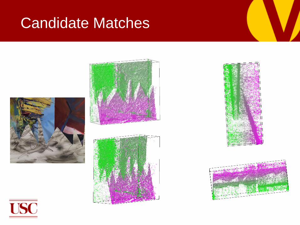
Candidate Matches

Tensor Voting
Tokens initialized at
locations of initial
matches
■As balls if no prior
information is available
Cast first and second
order votes to neighborsx
y
d
OR
vx, vy
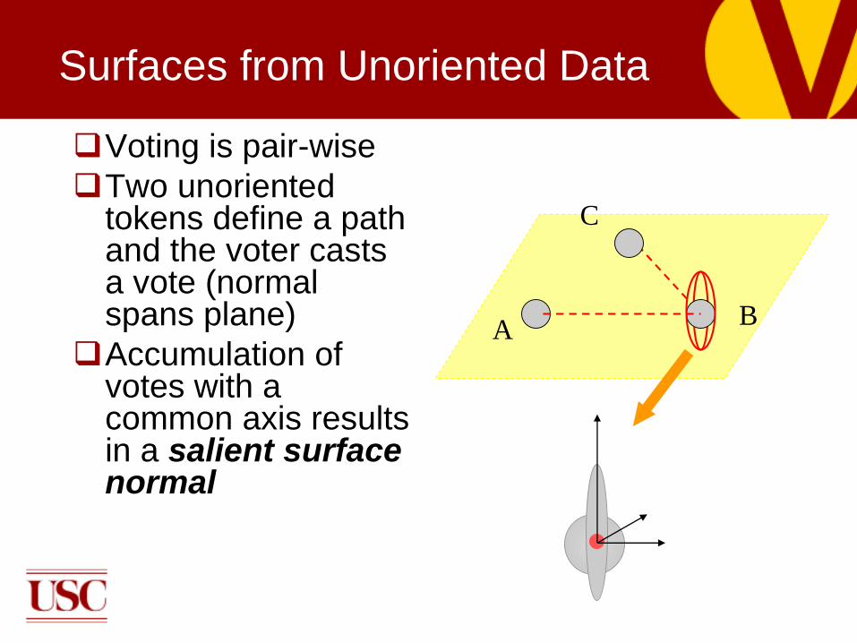
Surfaces from Unoriented Data
Voting is pair-wise
Two unoriented tokens define a path and the voter casts a vote (normal spans plane)
Accumulation of votes with a common axis results in a salient surface normal
A
C
B

Uniqueness
Tokens are classified according to saliency
and polarity
Most salient token along each Line of Sight
is retained
■Disambiguation of initial matches
Outliers rejected based on low saliency

Uniqueness vs. Visibility
Uniqueness constraint: One-to-one pixel
correspondence
■Exact only for fronto-parallel surfaces
Visibility constraint : M-to-N pixel
correspondences
■[Ogale and Aloimonos 2004][Sun et al. 2005]
■One match per ray of each camera
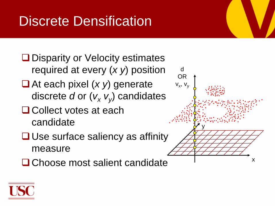
Discrete Densification
Disparity or Velocity estimates
required at every (x y) position
At each pixel (x y) generate
discrete d or (vx vy) candidates
Collect votes at each
candidate
Use surface saliency as affinity
measure
Choose most salient candidate
d
OR
vx, vy
x
y

Results: Tsukuba
Ground truth
Error Map
Disparity MapLeft image
NEW Middlebury Evaluation
Error Rate 3.79%
Rank (at 1.0) 9
Rank (at 0.5) 11

Results: Venus
Left imageDisparity Map
Error Map
Ground truth
NEW Middlebury Evaluation
Error Rate 1.23%
Rank (at 1.0) 4
Rank (at 0.5) 1
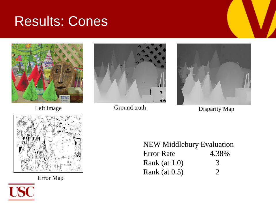
Results: Cones
Error Map
Disparity MapLeft image Ground truth
NEW Middlebury Evaluation
Error Rate 4.38%
Rank (at 1.0) 3
Rank (at 0.5) 2

Results: Teddy
Left image Ground truth
Error Map
Disparity Map
NEW Middlebury Evaluation
Error Rate 9.76%
Rank (at 1.0) 5
Rank (at 0.5) 3

Summary of Approach to Stereo
Binocular and monocular cues are combined
Novel initial matching framework
No image segmentation
Occluding surfaces do not over-extend because
of color consistency requirement
Textureless surfaces are inferred based on
surface smoothness
■ When initial matching fails

Overview
Tensor Voting in 2-D
Tensor Voting in 3-D
Applications to Computer Vision
■Figure Completion
■Stereo
■Motion
Tensor Voting in N-D
Probabilistic Tensor Voting

Monocular vs. Motion Cues
Structure inference possible from one image only…?
…or from motion only ?

Computational Processes
Matching■ Establish token correspondences across images
■ Recover a (possibly sparse and noisy) velocity fieldby Tensor Voting in 4-D (x, y, vx, vy)
Motion capture■ Obtain a dense representation :
■ Dense velocity field
■ Boundaries
■ Regions
Token Affinity
At the perceptual level – token affinity
In matching:
Preference for a certain correspondence
In motion capture:
Preference for grouping with other tokens, into a certain
region
Computationally – how to implement a measure of
token affinity ?

4-D Voting Approach
Layered 4-D representation
Match: (x y) (x+vx y+vy)
Represent each candidate match as a (x y vx vy) point in 4-D
Spatial separation in both image and velocity space
A
C
D
B
C
A
BD

4-D Voting Approach
Voting-based token communication
■Motion layers smooth surfaces in the 4-D space
■Affinity preference for being incorporated into a smooth layer
■Encourage affinity propagation:
within layers
■Inhibit affinity propagation:
across layers
at isolated pointsM. Nicolescu, G. Medioni, “Layered 4D Representation and Voting for Grouping from Motion”,
IEEE Transactions on Pattern Analysis and Machine Intelligence, 2003.

Extension to 4-D
Feature 1 2 3 4 e1 e2 e3 e4 Tensor
Point 1 1 1 1 Any orthonormal basis Ball
Curve 1 1 1 0 n1 n2 n3 t C-Plate
Surface 1 1 0 0 n1 n2 t1 t2 S-Plate
Volume 1 0 0 0 n t1 t2 t3 Stick
Elementary tensors
Feature Saliency Normals Tangents
Point 4 none none
Curve 3 - 4 e1 e2 e3 e4
Surface 2 - 3 e1 e2 e3 e4
Volume 1 - 2 e1 e2 e3 e4
A generic tensor
Implementation
Data structures – Approximate nearest
neighbor (ANN) k-d tree
Space complexity: O(n)
Time complexity (average): O(n)
n = number of input tokens
= average number of tokens in the
neighborhood

Matching Overview
Sparse voting
Correct matches (sparse)
Generating candidate matches
(x y vx vy) points in 4-D
Tensor encoding
4-D ball tensors
Affinity propagation
4-D generic tensors
Selection
(x y vx vy) points in 4-D
M. Nicolescu, G. Medioni, “Perceptual Grouping from Motion Cues Using Tensor Voting in 4-D”,
European Conference on Computer Vision, 2002.

Generating Candidate Matches
Establish a potential match with all tokens in a
neighborhood
Input frames:
sparse identical point tokens
motion cues only
Candidate matches:
(x y vx vy) points in 4-D

Affinity Propagation
Sparse voting process start with ball tensors
Enforce smoothness of motion layers
Token communication strong within layers, weak across
layers, weak at isolated tokens
x
y
vx, vy
x
y
vx, vy

Selection
Wrong matches appear as outliers, receiving
little or no support
Affinity (support) is expressed by the surface
saliency at each token: 2 - 3
Sparse velocity field Recovered vx velocities
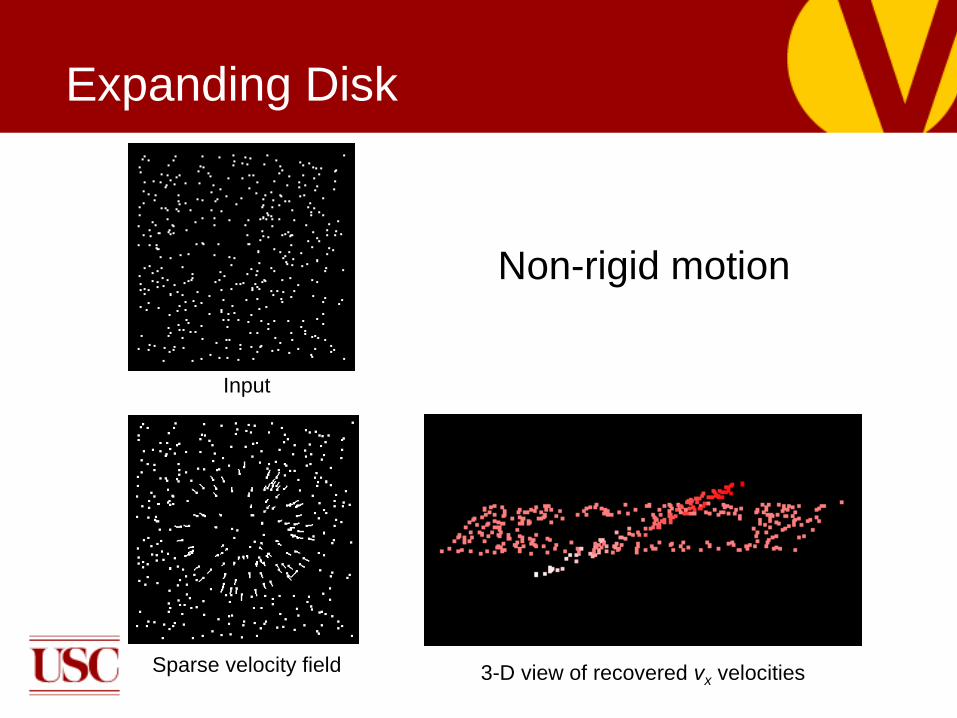
Expanding Disk
Non-rigid motion
Sparse velocity field 3-D view of recovered vx velocities
Input

Expanding Disk
Regions Boundaries
Dense velocity field
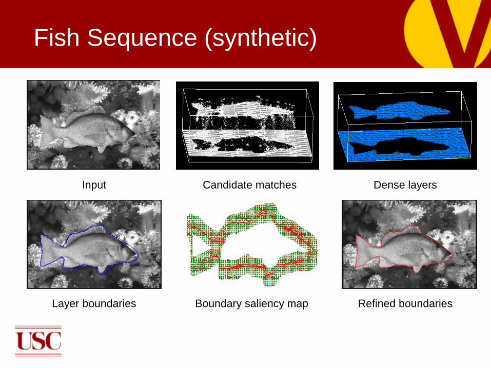
Fish Sequence (synthetic)
Dense layersCandidate matchesInput
Refined boundariesBoundary saliency mapLayer boundaries
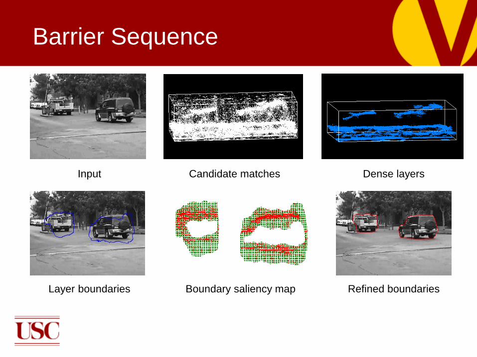
Barrier Sequence
Dense layersCandidate matchesInput
Refined boundariesBoundary saliency mapLayer boundaries

3-D Interpretation
Goal:
■Given 2 views of a scene, recover the 3-D structure
and motion
Possible interpretation processes:
■Structure from motion interpret changing
projections of unrecognized objects in motion
■Motion from structure use recognized 3-D
structure to derive motion

Difficulties
■Inherent ambiguity of 2-D 3-D interpretation
Add rigidity constraint
■General motion (multiple independent motions, non-rigid motions)
Global constraint – difficult to handle misfits (outliers, non-rigid, or independent motion?)
Decouple processes of matching, outlier rejection, grouping and interpretation
Segment objects and eliminate outliers based on motion smoothness, then locally enforce rigidity for each object
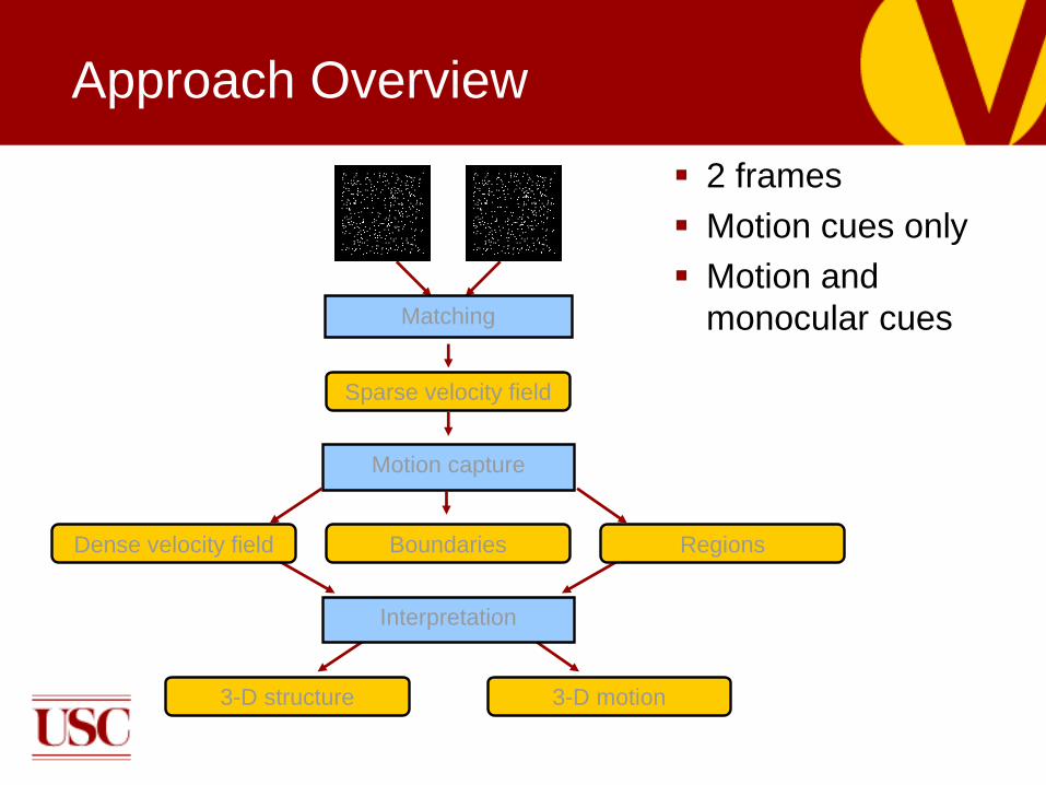
Approach Overview
Matching
Sparse velocity field
Motion capture
Interpretation
Dense velocity field Boundaries Regions
3-D structure 3-D motion
2 frames
Motion cues only
Motion and
monocular cues

The Rigidity Assumption
■Consistent with human perception
rigid 3-D interpretation whenever possible
Possible rigidity
Necessary non-rigidity

Approach
Matching
Outlier rejection
Grouping
. . .
Rigidity test
O1 ON
O1 OK. . . O1 ON. . .
3-D reconstruction
S1 SK. . .
rigid non-rigid
Motion
analysis
Motion
interpretation
3-D structure and motion

Rigidity Test
■ McReynolds and Lowe ’96: verify potential rigidity of minimum
6 point correspondences in 2 frames
Multiple rigid motions
Single rigid motion
Non-rigid motion

3-D Reconstruction
For each rigid subset of matches:
■Estimate epipolar geometry (RANSAC)
fundamental matrix
■Compute camera/object 3-D motion camera
matrices
■Recover 3-D structure
No reconstruction attempted for non-rigid
objects
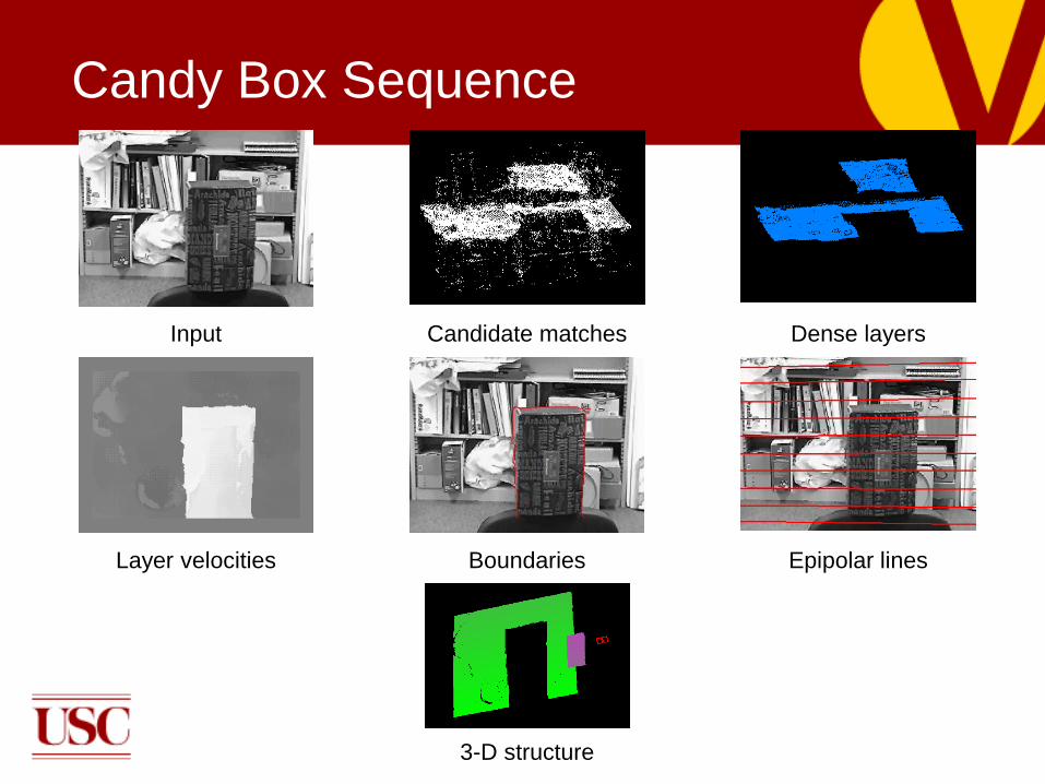
Candy Box Sequence
Dense layersCandidate matchesInput
Epipolar linesBoundariesLayer velocities
3-D structure

Books Sequence
Dense layersCandidate matchesInput
Epipolar linesBoundariesLayer velocities
3-D structure

Car Sequence
Dense layersCandidate matchesInput
Epipolar linesBoundariesLayer velocities
3-D structure

Cylinders Sequence
VelocitiesCandidate matchesInput
3-D structureDense layers

Flag Sequence
VelocitiesCandidate matchesInput
Dense layers (vx) Dense layers (vy) Dense sequence
(reconstructed)

Overview
Tensor Voting in 2-D
Tensor Voting in 3-D
Applications to Computer Vision
■Figure Completion
■Stereo
■Motion
Tensor Voting in N-D
Probabilistic Tensor Voting

Unified Tensor Voting
Input data are points in RD
Inliers lie on a low dimensional manifold
embedded in RD
Unobserved data also lie on the manifold
TV estimates manifold’s tangent/normal space
and intrinsic dimensionality locally
Instance based Machine Learning

Manifold Structure Learning
Related Work■ Non-Robust Methods
Local PCA, [Zhang and Zha, 2004]
Local Factor Analysis (LFA) [Teh and Roweis, 2003]
Kernel PCA, [Mika and Scholkopf and et al, 1999]
Local Smooth Manifold Learning, [Dollar, Rabaud and Belongie, 2007]
■ Robust Methods
Robust Subspace Learning (RSL) [Torre and Black, 2003]
• Non-convex
Robust PCA [Wright, Peng, Ma and Candés, 2009, 2010]
• Lack out-of-sample extension
ND-TV [Mordohai and Medioni, 2010]

Overview
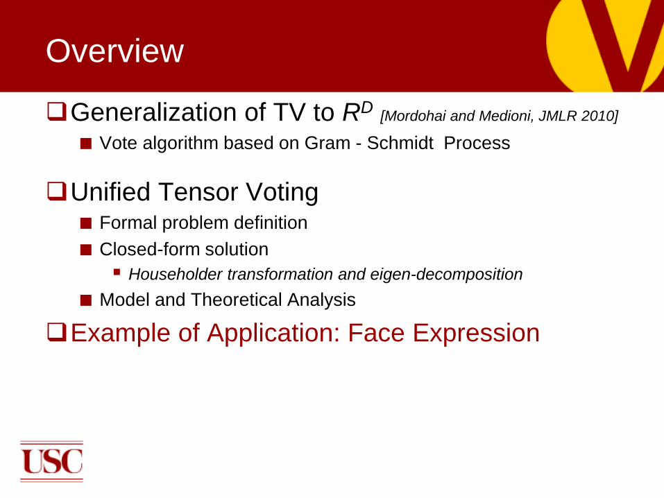
Generalization of TV to RD[Mordohai and Medioni, JMLR 2010]
■ Vote algorithm based on Gram - Schmidt Process
Unified Tensor Voting■ Formal problem definition
■ Closed-form solution
Householder transformation and eigen-decomposition
■ Model and Theoretical Analysis
Example of Application: Face Expression

Tensor Voting in N-D
Direct generalization of 2-D and 3-D cases
■Tensors become second order, N-dimensional,
symmetric, non-negative definite
■Polarity vectors become N-D vectors
■There are N+1 structure types (0-D junction to
N-D hyper-volume)
Bottleneck: N second order and N first order
fields are required
■Storage and computation requirements grow
exponentially with N

Limitations of Voting Fields
Cannot generalize to N dimensions
Requirements: N N-D fields
■k samples per axis: O(NkN) storage requirements
■Nth order integration to compute each sample: O(kd) computations per sample
S(P) B(P)
PP
dPP )()( SB

Problem Definition
From Manifold to Tensor (2nd order)
■ Given (sub) manifold M (intrinsic dimension d) embedded in RD
• How to encode the geometric information at x?
Dual formulation
normal space associated with non-zero constant eigenvalues
tangent space associated with zero eigenvalues
1
dT T
i ik
T u u U U
T is invariant representation of a subspace !
Positive Semidefinite Cone
1
'D d
Ti i
k
T v v
( , )Gr d DGrassmannian manifold
Intrinsic dimensionality: d(D-d)

Problem Definition
Examples
■ Tensors can encode all structure types simultaneously
D+1 types of structure in RD space
■ Robust representation of the local geometric structure
1 0 0
0 1 0
0 0 0D D
1 0 ... 0
0
0
0 ... 0 1D D
d=1 Manifold D-dimensional points
Features

Direct Vote Computation
Arbitrary tensors decomposed in N basic
tensors
Vote generation from unit stick is the same
Voter, receiver and voting stick define a 2-D plane
in any dimension
Other components cast direct votes
Explained later

Tensor Representation in N-D
Tensor construction:
■eigenvectors of normal space associated with
non-zero eigenvalues
■eigenvectors of tangent space associated with
zero eigenvalues
Tensor still represent all structure types
simultaneously
Noise robustness is the same
■Higher than other methods

Vote Analysis
Tensor decomposition:
Dimensionality estimate: d with max{λd- λd+1}
Orientation estimate: normal subspace
spanned by d eigenvectors corresponding to d
largest eigenvalues
d
T
ddN
TTT
T
NNN
TT
eeeeeeee
eeeeee
...))(()(
...
2211321121
222111T

Results of Vote Analysis
At each point:
■Dimensionality estimate
■Normal subspace
■Tangent subspace
Linear constraints provided by local normal
and tangent subspaces
■Derivatives can be estimated

Recall the Standard Framework■ Stick fields and ball fields are defined separately in the 2-D
framework
■ Use stick field to generate other fields in high dimensional space
(integration)
Problem
Why does this cause problem for the tensor voting framework?
S(P) B(P)
Conflict with the linearity property!

Idea 1: Is “integration” a good idea?
Problem
+
Voter
Receiver
Option 1 Do linear
decomposition first
Option 2
The
integration idea
Different voting
results!

Problem
Idea 2: directly vote with ”natural eigenvectors”
■Non-unique issue for eigenvector
Non-unique voting results problem!

Problem
Idea 2: directly vote with ”natural eigenvectors”
■Is this a good idea?
A small noise is added to the tensor
Zero result,
due to 45o cut off
So, a small noise can lead to large difference !

Voting with eigenvectors is not a good idea
Stick and Ball (Integration) fields are
inconsistent■ Energy normalization, different results
Solution
■Directly derive ALL other fields from the
fundamental field by decomposition
■Use alignment process for voting
Problem

Our solution: there is no ball field!
Ball vote is derived from stick vote
Align basis vectors by the
link between voter and receiver
Only one vector votes
to the receiver
This is the idea used to derive the unified N-D Tensor Voting algorithm

Our solution
Step 1: do low-rank decomposition for a
tensor
Step2: design vote algorithm for each matrix
Step 3: sum up the results
+
rank-1 matrix rank-2 matrix
This is the idea used to derive the unified N-D Tensor Voting algorithm
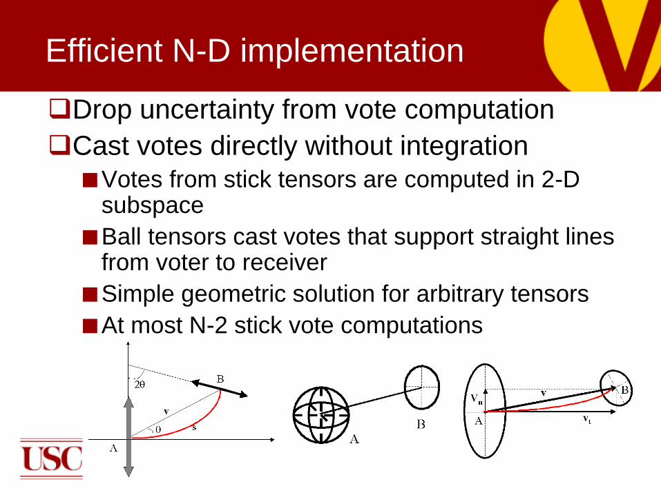
Efficient N-D implementation
Drop uncertainty from vote computation
Cast votes directly without integration
■Votes from stick tensors are computed in 2-D subspace
■Ball tensors cast votes that support straight lines from voter to receiver
■Simple geometric solution for arbitrary tensors
■At most N-2 stick vote computations
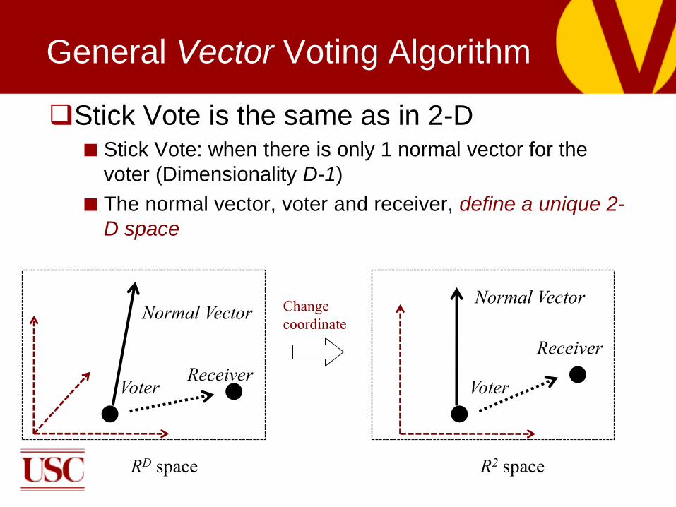
Stick Vote is the same as in 2-D■ Stick Vote: when there is only 1 normal vector for the
voter (Dimensionality D-1)
■ The normal vector, voter and receiver, define a unique 2-
D space
General Vector Voting Algorithm
RD space
VoterReceiver
Normal Vector
R2 space
Voter
Receiver
Normal VectorChange
coordinate

Stick Vote is the same as in 2-D■ Arc curve: this is the curve to minimize the curvature align the
curve, when θ is less than π/4
■ Voting weight: weight attenuates when distance increases and
angle increases
General Voting Algorithm
R2 space
Normal
Vector
Receiver2 2
2
( , )
( , ) exp( )
/ sin( ), 2sin( ) /
sin(2 ) sin(2 )
cos(2 ) cos(2 )
B
T
T weight v R
s cweight v
s v v
R

General vote*
■ Decompose a tensor (N.N.D.) to low-rank matrix
■ Design a simple geometric algorithm for low-rank matrix, then
get weighted sum of all the voting results
General Voting Algorithm
Mordohai and Medioni, JMLR 2010*
Rank-1 Rank-2
1 1 1 2 2 2
1 2 1 1 2 3 1 1 2 2
...
( ) ( )( ) ...
T T TD D D
T T T TD d d
d
e e e e e e
e e e e e e e e
T
Illustration of Decomposition
Rank-D
1 2( ) 2 3( ) 3

General vote*■ Design a simple geometric algorithm for low-rank matrix
General Voting Algorithm
Mordohai and Medioni, JMLR 2010*
Rank-2
1 1 1 2 2 2
1 2 1 1 2 3 1 1 2 2
...
( ) ( )( ) ...
T T TD D D
T T T TD d d
d
e e e e e e
e e e e e e e e
T
Illustrations for
rank-2 vote when D=3
Assume e1 and e2
Span the y-z space
y
x
z
1e
2e
v

Illustration■ Key issue is to align the basis vectors
Step 1: Choose e2’ first
Step 2: Choose e1’, which is orthogonal to e2’
• Especially, e1’ is also orthogonal to v
Step 3: Sum up the votes based on e1’ and e2’
General Voting Algorithm
y
x
z
y
z
x
1e
2e1 'e
2 'e
v v
1 2
1
2
2 2
( , ) ,
( , )
'
' proj
when space e e v e can be chosen arbitr
e v e
l
e
ari y
How to vote?

Illustration■ The vote for this rank-2 matrix is based on the new basis
General Voting Algorithm
2 3 1 1 2 2
2 3 1 1 2 2
(( )( ))
( )[ ( ' ' ) ( ' ' )]
T T
T T
Vote e e e e
Vote e e Vote e e
y
x
z
y
z
x
1
2 1 2
cov( ', ) 0
cov( ', ) cov( ( , ), )
e v
e v space e e v
1e
2e1 'e
2 'e
v v
Basis Vectors
Re-decomposition

General Vote■ In general, the vote of a rank-d matrix is:
General Voting Algorithm
1 1 2 2
1 1 2 2
( ... )
( ' ' ) ( ' ' ) ... ( ' ' )
T T Td d
T T Td d
Vote e e e e e e
Vote e e Vote e e Vote e e
1
1
' : ' / , ( ,... )
: cov( , ) cov( ( ,... ), )
d d proj proj proj d
proj d
e is specially chosen as e v v v is the projection of v to space e e
so we have v v space e e v
Intuition: only ed’ is correlated to v, other basis vectors are all orthogonal to v, and
votes become very simple
1e je
de
1 'e'je
'de

Analysis for the General vote■ Choose a new basis
We can use Gram-Schmidt process, but…
The decomposition results are not unique
■ Voting Results
Invariant to the basis choosing process
The last basis vector is the key
General Voting Algorithm
1e je
de
1 'e
'je
'de
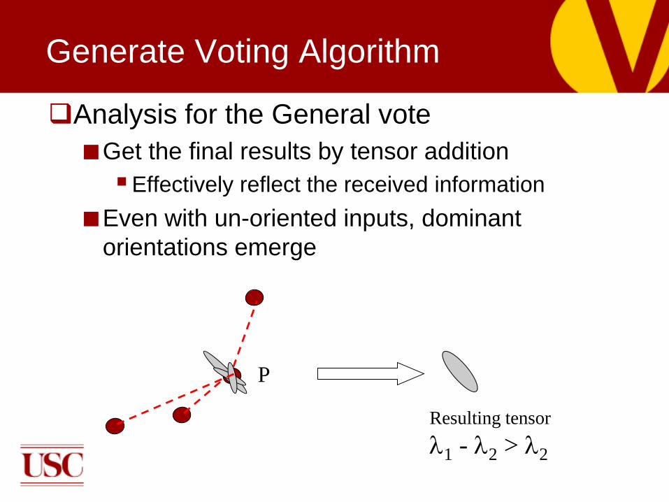
Generate Voting Algorithm
Analysis for the General vote
■Get the final results by tensor addition
Effectively reflect the received information
■Even with un-oriented inputs, dominant
orientations emerge
P
Resulting tensor
1 - 2 > 2

General Voting Algorithm
Special Cases of this unified framework■ Case 1: d=1 (normal space of dimension one)
No need for basis change, use e1 directly
Which is just the stick vote in previous framework
Recall the previous re-decomposition, since the normal space is a 1D space, so there is
no need for re-decomposition
1 1 1 1cov( , ) , ' /proj proj projSince v e v e so e v v e
Voter
Receiver
Normal Vector

Special Cases of this unified framework■ Case 2: d=D (normal space of dimension D)
We can prove the vote has an efficient computational formulation
Importantly, this case is applicable for raw input data,
when all tensors are initialized as identity matrixes
General Voting Algorithm
2 2exp( / )( )Tvvote s I vv
Recall the previous re-decomposition, since the normal space is the full space, so the
last basis vector is just v
1( ,... ) , , 'Dd proj DSince space e e R so v v and e v

General Voting Algorithm
Special Cases of this unified framework■ Case 3: 1<d<D (non-trivial case)
If cov(normal space, v) = 1
• Show that v is fully inside the normal space
• Turn to the same formulation in case 2 (but in the Rd space)
If cov(normal space, v) = 0
• This is a very special case, and the results are quite simple
• We can choose any basis, no need for decomposition
'de v 2 2
1
exp( / )( )d
T Tv j j
j
vote s e e vv
2 2
1
exp( / )d
Tv j j
j
vote s e e

Deriving a Closed Form solution
general vote is weighted sum of D low-rank matrix vote as
The stick vote (rank-1), i.e., the only fundamental vote, is

Closed Form (cont)
Furthermore, the weight kernel is decomposed into two factors
If the angle kernel function is non-increasing and convex with respect to < r,
e >, then it can be shown that the alignment method is equivalent to
maximizing the trace of the voting result.

Closed form (cont)

Closed form (end)
So finally we can get the closed form solution

Discussion
Key feature: there is no separate ball voting field, and in
fact, all voting functions are derived naturally from the stick
vote.
Thus, the problem of the inconsistency between the stick
and ball vote is solved elegantly.
Two special cases are given below

Comparison with Original Implementation
Tested on 3-D data
Saliency maps qualitatively equivalent
Old
New
Surface saliency
z=120
Surface saliency
z=120
Curve saliency
z=0

Comparison with Original Implementation
Surface orientation estimation
■Inputs encoded as ball tensors
Slightly in favor of new implementation
■Pre-computed voting fields use interpolation
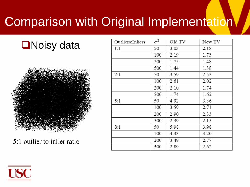
Comparison with Original Implementation
Noisy data
5:1 outlier to inlier ratio

Orientation Estimation: the
“Swiss Roll” example

High-Dimensional Data
Sample 3 or 4 variables
Generate 14 to 16 outputs as linear and
quadratic functions of those
Embed in high dimensional spaces with
noise

Data with Varying Dimensionality
Input: un-oriented points in 4-D
■ 1-D line
■ 2-D cone
■ 3-D hyper-sphere

Varying Dimensionality: Results
3- 4 is max
2- 3 is max

Varying Dimensionality: Results
1- 2 is max

Nonlinear Interpolation and
Manifold Distance Measurement
Do not reduce
dimensionality
Start from point on
manifold
Take small step along
desired orientation on
tangent space
Generate new point and
collect votes
Repeat until
convergence
AA1
B
p

Distance Measurement
Error in orientation estimation: 0.11o0.26o

Traveling on Manifolds
50-D30-D

Function Approximation
Tensor Voting on training set (both observed
and state variables)
Testing data have observed variables only
Find nearest neighbor in observed space
Generate samples on path towards desired
coordinates of test sample as before
Repeat if function has branches

Function Approximation Results
Noise-free Input
Schaal and Atkenson, 1998

Function Approximation Results
Goal: generate more samples of the function
and evaluate against ground truth
■Noise-free case
■With 5 times more outliers than inliers
■Add perturbation to data (incl. outliers)
■Embed to 60-D with outliers and perturbation
NMSE 0.0041 0.017 0.035 0.024

Advantages over State of the Art
More general applicability
■Manifolds with intrinsic curvature (cannot be unfolded)
■Non manifolds (spheres, hyperspheres)
■Intersecting manifolds
■Data with varying dimensionality
Reliable dimensionality estimation at point level
No global computations O(NM logM)
Noise Robustness
Overview
Generalization of TV to RD[Mordohai and Medioni, JMLR 2010]
■ Vote algorithm based on Gram - Schmidt Process
Unified Tensor Voting■ Formal problem definition
■ Closed-form solution
Householder transformation and eigen-decomposition
■ Model and Theoretical Analysis
Example of Application: Face Expression

Overview
Facial Deformations Head Pose
Recognition and
Interpretation
Expressions, Facial Gestures
Training Database
Face Sequences
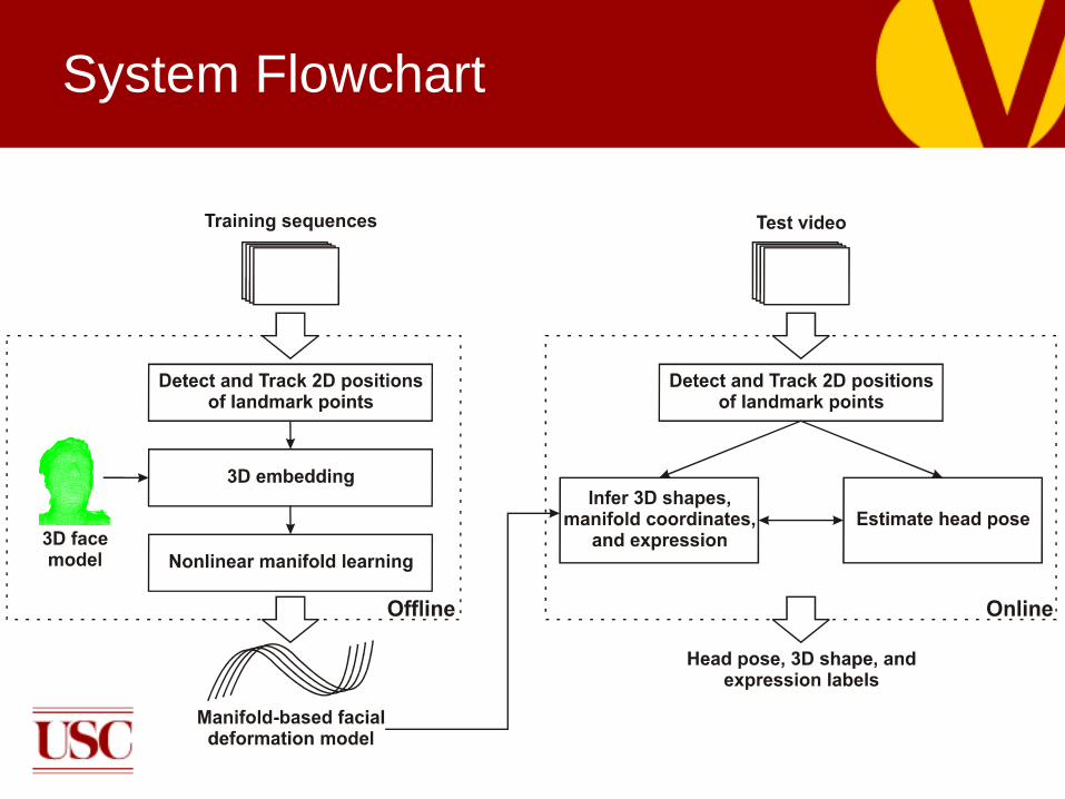
System Flowchart

3D Face Shape
Use 42 landmark points to represent face shape
An instance of nonrigid facial deformation is represented by a
42 x 3 = 126 dimensional vector
High dimensional space
■ Explore intrinsic structure / manifolds of facial deformations
2D projection 3D frontal 3D non-frontal

1D Manifolds
% of
1D
Surprise 90.1%
Anger 85.3%
Joy 93.4%
Disgust 95.3%
Sadness 90.1%
Close eyes 88.7%
Blinking – left 92.4%
Blinking – right 93.9%

Traversing the Manifold with
Tangent Vectors
X1
X2X3
X̂
H0 ← Tensor Voting
X
D0 ← H0H0T(X – X0)X1 ← X0 + α0D0
H1 ← Tensor VotingD1 ← H1H1T(X – X1)X2 ← X1 + α1D1
H2 ← Tensor Voting
D2 ← H2H2T(X – X2)
X3 ← X2 + α2D2
H3 ← Tensor Voting
D3 ← H3H3T(X – X3)
X4 ← X3 + α3D3
X0
X4 optimal projection of X

Video Results

Results – Surprise
Probability of other
expressions

Results – Smile
Probability of other
expressions

Future Directions
Currently, we learn person-dependent manifolds
■ Generalize to person-independent manifold
■ Use generic face model
Number of manifoldsHow many manifolds are required to cover all possible
facial deformations?
Are these manifolds independent of each other?
■ Minimum number of manifolds to cover facial deformations
■ Indicate number of basic/primitive expressions
Synthesis

Overview
Tensor Voting in 2-D
Tensor Voting in 3-D
Applications to Computer Vision
■Figure Completion
■Stereo
■Motion
Tensor Voting in N-D
Probabilistic Tensor Voting

Probabilistic Tensor Voting
So far, we assume that tokens are accurately
located, (or are outliers)
In practice, the data itself contains Gaussian
noise
The new problem becomes
Inference of multiple manifolds in the
presence of Gaussian and Outlier noise
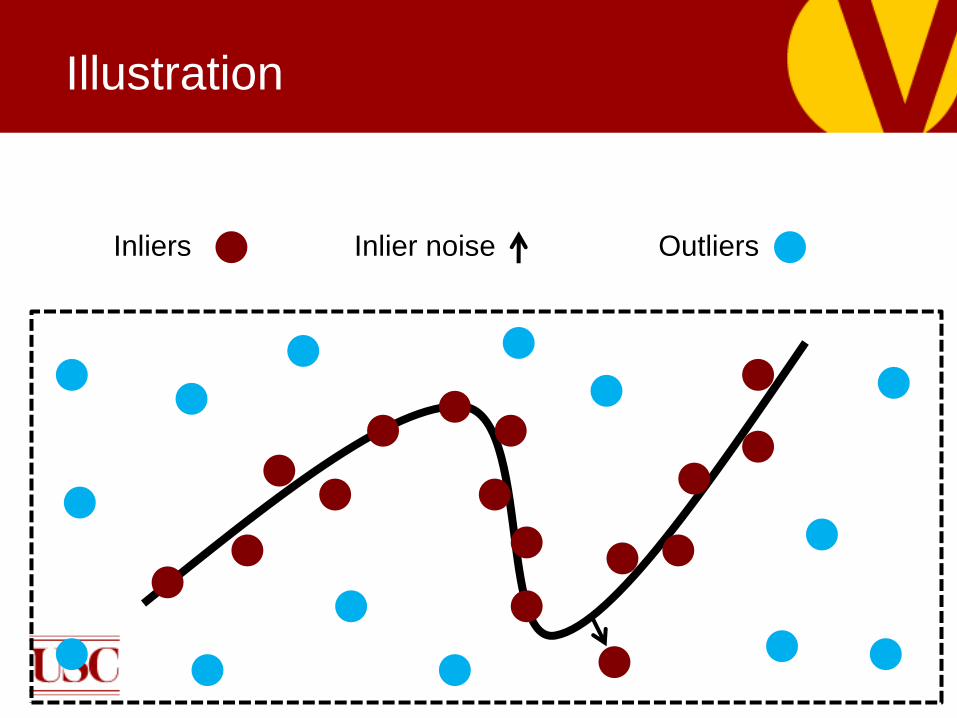
Inliers Inlier noise Outliers
Illustration

Problem
This is common
■Dense voting in R2, position noise for points
sampled from a manifold

Problem
Current Voting scheme is sensitive when two
points are close
What if
voter’s
position shifts
a little?
Voting results
A large change of orientation due to a very small change
in the position with high confidence (voting saliency)
voting
voting

Geometry meets Uncertainty
Introduce uncertainty in the voter’s position
Distribution is assumed to be Gaussian
Prior distribution is learnt from the data
■The support space of the prior is learnt
■Noise magnitude is another parameter of the
algorithm: noise voting scale
Gong and Medioni, 2011

Probabilistic Tensor Voting
Related Work■ Kernel Principal Component Analysis (KPCA)
[Mika and Scholkopf and et al, NIPS 1999]
■ Robust Principal Component Analysis (RPCA)
[De la Torre and Black, IJCV 2003]
■ RANSAC / StaRSac [Choi and Medioni, CVPR 2009]
■ Manifold based Nonlinear Dimension Reduction (NLR)
■ Locally Smooth Manifold Learning (LSML)
[Dollar, Rabaud and Belongie, NIPS 2007]
■ Diffusion Map based Manifold Denoising (DM-MD)
[Hein and Maier, NIPS 2007]
■ N-D Tensor Voting [Mordohai and Medioni, JMLR 2010]
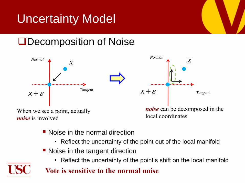
Decomposition of Noise
Noise in the normal direction
• Reflect the uncertainty of the point out of the local manifold
Noise in the tangent direction
• Reflect the uncertainty of the point’s shift on the local manifold
Uncertainty Model
Normal
Tangent
x
x
Normal
Tangent
x
x
When we see a point, actually
noise is involved
noise can be decomposed in the
local coordinates
Vote is sensitive to the normal noise

Vote with uncertainty
Voting results from a vector become a matrix
New fundamental field is generated numerically
( ) ( )nStick
x normal space
Vote T x p x dx
Probabilistic Vote
jx
ix
Standard
Stick Vote
jx
ix
Probabilistic
Stick Vote
s
l
noise voting scale

PTV Voting Field
Comparisons
STV PTV

PTV Voting Field
Two views visualization
PTVPTV

Summary
the 1st pass vote is used to estimate the local geometric
structure, the 2nd pass vote is used to refine estimations
and the 3rd pass is used to generate unobserved data
Estimate structure and filter out outliers
Robust to two parameters
Requires
New fundamental field
vote noiseand
vote noise

Overview
Standard Tensor Voting
Application to Computer Vision
Problems of the Standard Framework
Unified N-D Tensor Voting Framework
Probabilistic Tensor Voting
■New fundamental field
■Polarity Vectors and Polarity Vote
■General Probabilistic Voting Algorithm
Conclusion

Polarity Vote
So far, we focus on 2nd order information■ It is not enough in some cases
Need First Order Information■ Tensor is robust representation
■ But insensitive to signed information
■ Polarity vote in the Standard Framework
Based on the second order tensor
Reflect the asymmetric properties
Problems: only one type of asymmetry
A
B
C
, . . ?A B v s C
jx
ix
2nd order
1st order

2 Polarities Vote
Now, we have two types of polarity vector
Type 1 polarity vector■ Asymmetry of the manifold sampling
■ Detects endpoints
Type 2 polarity vector■ Asymmetry of the local manifold
■ Points to the manifold
jx
ix
1type polarity
2type polarity

Polarity Votes
How to vote to get two polarity vectors
Voting saliency is the same as that in the second order
case
Polarity votes are based on the second order
information (initialized as zero)
Accumulated by vector addition2 2
2( , ) exp( ),
s cweight v the same as before
Voter
Normal direction
1 . .type P V 2 . .type P V
Vector Addition
Polarity Votes
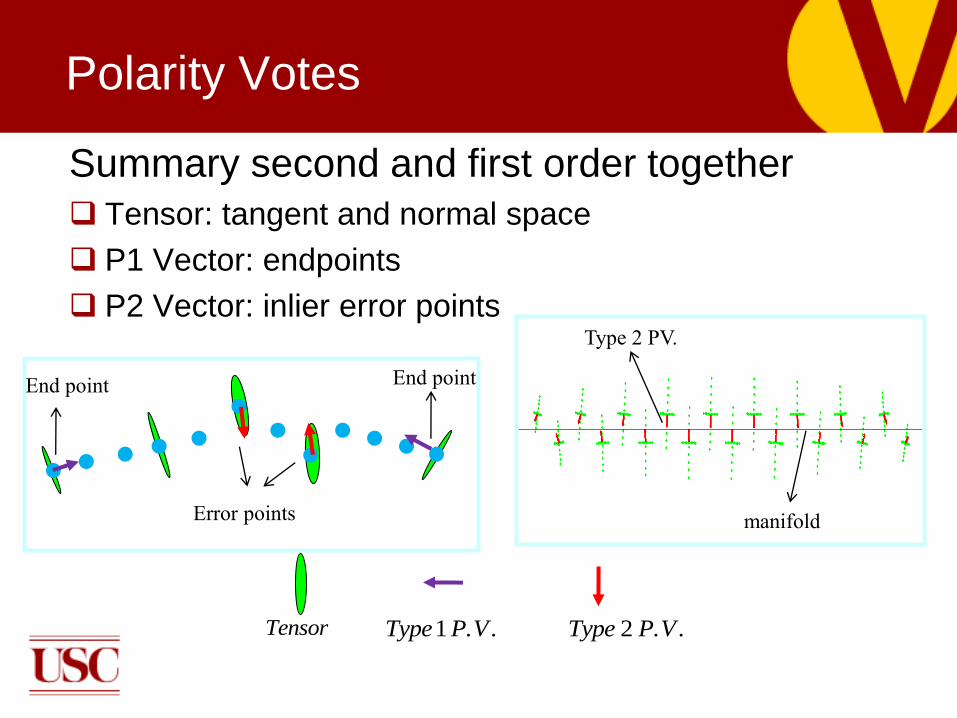
Summary second and first order together
Tensor: tangent and normal space
P1 Vector: endpoints
P2 Vector: inlier error points
Tensor 2 . .Type P V1 . .Type P V
End point End point
Error points manifold
Type 2 PV.
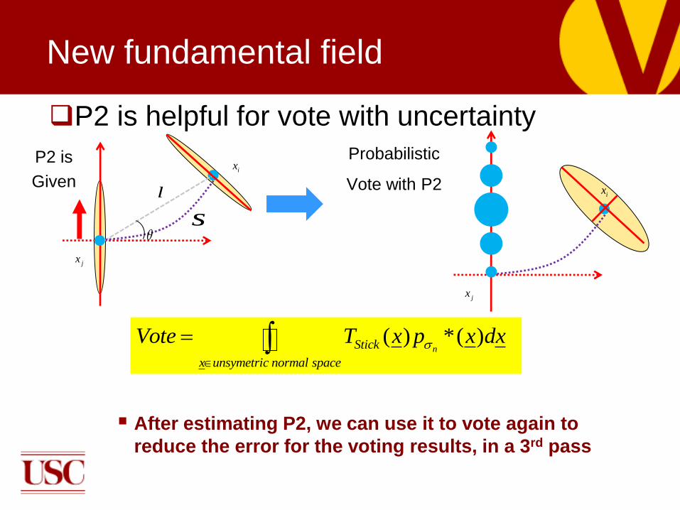
P2 is helpful for vote with uncertainty
After estimating P2, we can use it to vote again to
reduce the error for the voting results, in a 3rd pass
( ) *( )nStick
x unsymetric normal space
Vote T x p x dx
New fundamental field
jx
ixP2 is
Given
jx
ix
Probabilistic
Vote with P2
s
l

Results
Endpoint Completion■ A dense voting case, synthetic error on endpoint’s position
■ Three passes votes, P2 is used to refine the vote
Standard voting New voting
2 . .Type P V1 . .Type P V
Results
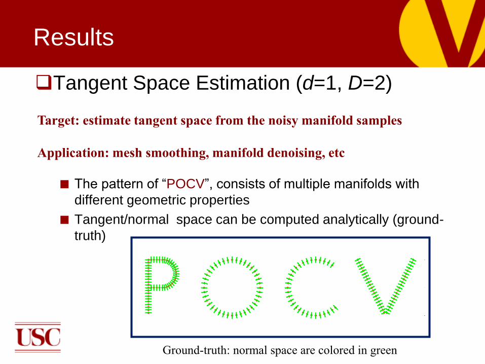
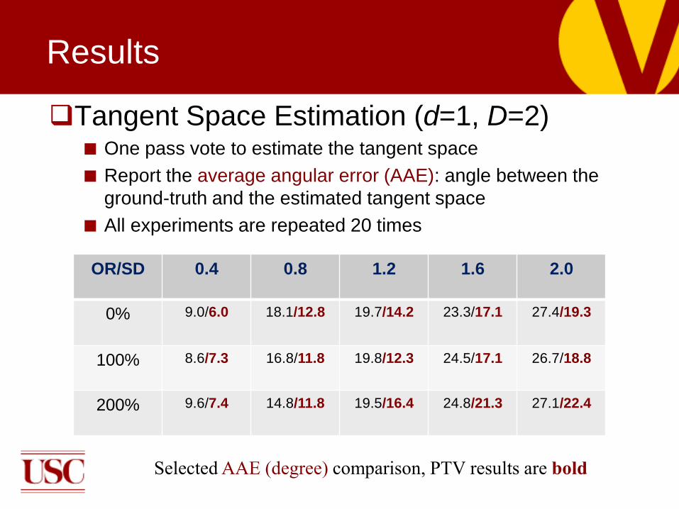
Tangent Space Estimation (d=1, D=2)
■ The pattern of “POCV”, consists of multiple manifolds with
different geometric properties
■ Tangent/normal space can be computed analytically (ground-
truth)
Target: estimate tangent space from the noisy manifold samples
Application: mesh smoothing, manifold denoising, etc
Ground-truth: normal space are colored in green

Results
Tangent Space Estimation (d=1, D=2)■ Add different levels of position Gaussian noise on inlier, add
different amount of outlier noise (uniformly distributed)
OR = outlier ratio = # of outliers / # of inliersSD = standard derivation of position noise
OR/1
SD/0
OR/2
SD/1
OR/2
SD/2
OR/1
SD/0.5
Results
Tangent Space Estimation (d=1, D=2)■ One pass vote to estimate the tangent space
■ Report the average angular error (AAE): angle between the
ground-truth and the estimated tangent space
■ All experiments are repeated 20 times
OR/SD 0.4 0.8 1.2 1.6 2.0
0% 9.0/6.0 18.1/12.8 19.7/14.2 23.3/17.1 27.4/19.3
100% 8.6/7.3 16.8/11.8 19.8/12.3 24.5/17.1 26.7/18.8
200% 9.6/7.4 14.8/11.8 19.5/16.4 24.8/21.3 27.1/22.4
Selected AAE (degree) comparison, PTV results are bold

Tangent Space Estimation (d=1, D=2)■ Results are robust to the choice of noise voting scale
Relative Error (RE) = Error of PTV / Error of STV
OR=1 SD=1
noise
RE10vote

Results
More cases: sphere data (d=2, D=3)■ Different levels of inlier and outlier noise
■ Color of inliers and outliers different for visualization purposes
PTV decreases the error by 10% on average

Inference of Global Manifold Properties using the Tensor Voting Graph
Gérard Medioni
Work with Shay Deutsch

Tensor Voting limitations
Tensor Voting is a strictly local
method: global operations are not
easy
Geodesic using iterative approach
■ Diverge on deep concavities:
■ Slow and not efficient
Clustering is not reliable
-15
-10
-5
0
5
10
15
-15
-10
-5
0
5
10
15
0
50
O
P
AA1
B
p
The Tensor Voting Graph
Key Idea: construct a graph which diffuses the local information of the tensor votes
Infer the manifold global structure: overcome TV main limitation
Reversed tensor votes: contribution that was made to its local tangent space during the voting process
Affinity is based on the normal spaces and the reversed tensor votes

Tensor Voting Graph
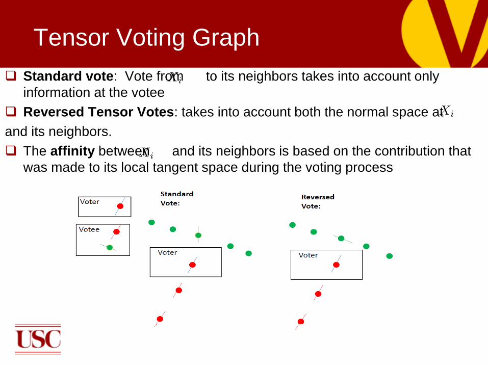
Tensor Voting Graph
Standard vote: Vote from to its neighbors takes into account only
information at the votee
Reversed Tensor Votes: takes into account both the normal space at
and its neighbors.
The affinity between and its neighbors is based on the contribution that
was made to its local tangent space during the voting process

Experimental results: geodesic
distance estimation (with outliers)
Experimental Results with 100% outliers
• Tensor Voting graph defines the local neighborhood
• Compare using avg. geodesic distance error (all pairwise
points)

Quantitative results

Experimental results: geodesic distances
(intersecting manifold)
Experimental Results on self-intersecting Viviani's curve

Experimental results on real data:
motion segmentation
Segmenting a video sequence of multiple rigidly
moving objects into multiple clusters
Dataset: The 155 motion segmentation
benchmark

Motion segmentation results with
outliers
• Comparison to SSC
• Different amount of outliers noise
• randomly selected point
trajectories, which correspond to
20%,25%,30%,35%,40% of the
data, and corrupt 80% trajectories
entries with outliers noise

Explicit junction handling
Clustering Multiple Intersecting
Manifolds is a challenging problem
Local intersection area highly
ambiguous
Small maximal principal angles make
clustering is harder
Very disruptive to the entire clustering
process.

Multiple Intersecting Manifolds Linear intersecting manifolds
■ Generalized PCA (Vidal et al, 2003)
■ SSC(Elhamifar and Vidal, 2009)
For non-linear intersecting, few related method:
■ Multi-manifold semi-supervised learning,
(Goldberg, Zhu, Singh, Xu, Nowak, AISTATS 2009)
■ SMMC, (Wang, 2011)
■ RMMSL, D.Gong and G.Medioni (ICML 2012)
■ Local PCA based on Spectral Clustering(E Arias-Castro, 2013)
Common properties:
■ Use a measure of local tangent space distance to construct an affinity matrix
■ Spectral Clustering to partition the data
Limitations:
Perform well only when the maximal principal angle is large
Sensitive to outliers
Do not address the local intersection area explicitly

Experimental Results on challenging cases
(small principal angles)
Local intersection area: small portion, very disruptive!
Total Tangent space error:

Our approach
Resolve the ambiguities in the local
intersection area explicitly
Can handle manifolds with small principal
angles between the tangent spaces
Robust to a large amount of outliers

Overview

Delineation of the smooth manifolds parts
Estimate the local geometric
structure at each point
Identify the local intersection area
In the local intersection area:
normal votes are inconsistent

Intersecting Manifolds: Ambiguity
Resolution

Experimental Results: with 100% outliers

Experimental Results: manifolds
embedded in 50D
Randomly sample input variables
(2 and 3D intrinsic dimension
manifolds)
Map them to higher dimensional
vector
Summary
Tensor Voting Graph captures global
properties of the manifolds, using reversed
votes
Handles noise, non-linearity and intersection
Performs segmentation and grouping
Explicit junction handling

Contributions
General, expandable computational
framework
Unified and rich representation for all
potential types of structure and outliers
Efficient local information propagation
through Tensor Voting
No hard decisions until all information has
been considered