lecture # 07: laminar and turbulent flowshuhui/teaching/2014sx/class-notes/aere344... ·...

Copyright © by Dr. Hui Hu @ Iowa State University. All Rights Reserved!

Dr. Hui Hu

Department of Aerospace EngineeringIowa State University

Ames, Iowa 50011, U.S.A

Lecture # 07: Laminar and Turbulent Flows

AerE 344 Lecture Notes


Reynolds’ experiment

DU

Re


Laminar Flows and Turbulence Flows

• Laminar flow, sometimes known as streamline flow, occurs when a fluid flows in parallel layers, with no disruption between the layers. Inflow dynamics laminar flow is a flow regime characterized by high momentum diffusion, low momentum convention, pressure and velocity almost independent from time. It is the opposite of turbulent flow.

– In nonscientific terms laminar flow is "smooth," while turbulent flow is "rough."

• In fluid dynamics, turbulence or turbulent flow is a fluid regime characterized by chaotic, stochastic property changes. This includes low momentum diffusion, high momentum conversation, and rapid variation of pressure and velocity in space and time.

– Flow that is not turbulent is called laminar flow


Turbulent Flows in a Pipe

VD

Re


Characterization of Turbulent Flows

'';' wwwvvvuuu

Tt

t

Tt

t

Tt

t

dttzyxwT

wdttzyxvT

vdttzyxuT

u0

0

0

0

0

0

),,,(1;),,,(1;),,,(1


Turbulence intensities

0'0';0' wvu

0)'(0)'(;0)'(1)'( 2222

0

wvdtuT

uTt

t

o


Turbulent Shear Stress

yu

lam

Laminar flows:

''vuyu

turblam

Turbulent flows: ''vuturb

A.laminar flow b.turbulent flow



AU

DCd2

21

DU

Re


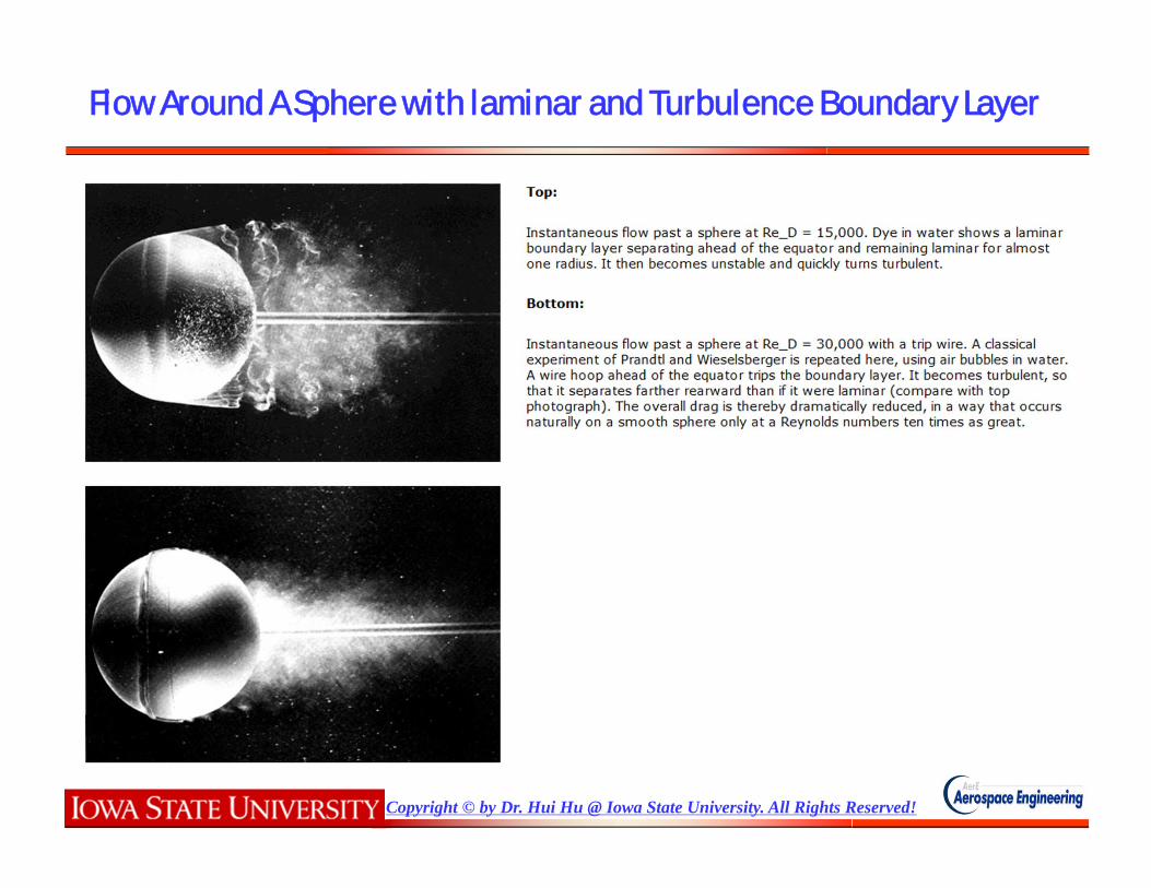
Flow Around A Sphere with laminar and Turbulence Boundary Layer


Aerodynamics of Golf Ball

Copyright © by Dr. Hui Hu @ Iowa State University. All Rights Reserved!X/D

Y/D

-101234

-1

0

1

2

U m/s: -10 -5 0 5 10 15 20 25 30 35 40

X/D

Y/D

-101234

-1

0

1

2 U m/s: -10 -5 0 5 10 15 20 25 30 35 40

X/D

Y/D

-101234

-1

0

1

2 U m/s: -10 -5 0 5 10 15 20 25 30 35 40

Smooth ball Rough ball Golf ball

-0.4

-0.2

0

0.2

0.4

0.6

0.8

1.0

-2.0 -1.5 -1.0 -0.5 0 0.5 1.0 1.5 2.0 2.5 3.0 3.5 4.0

smooth-ballrough-ballgolf-ball

Distance (X/D)

Cen

terli

ne V

eloc

ity (U

/U)


Re=100,000


Automobile aerodynamics


Automobile Aerodynamics

Mercedes Boxfish Vortex generator above a Mitsubishi rear window


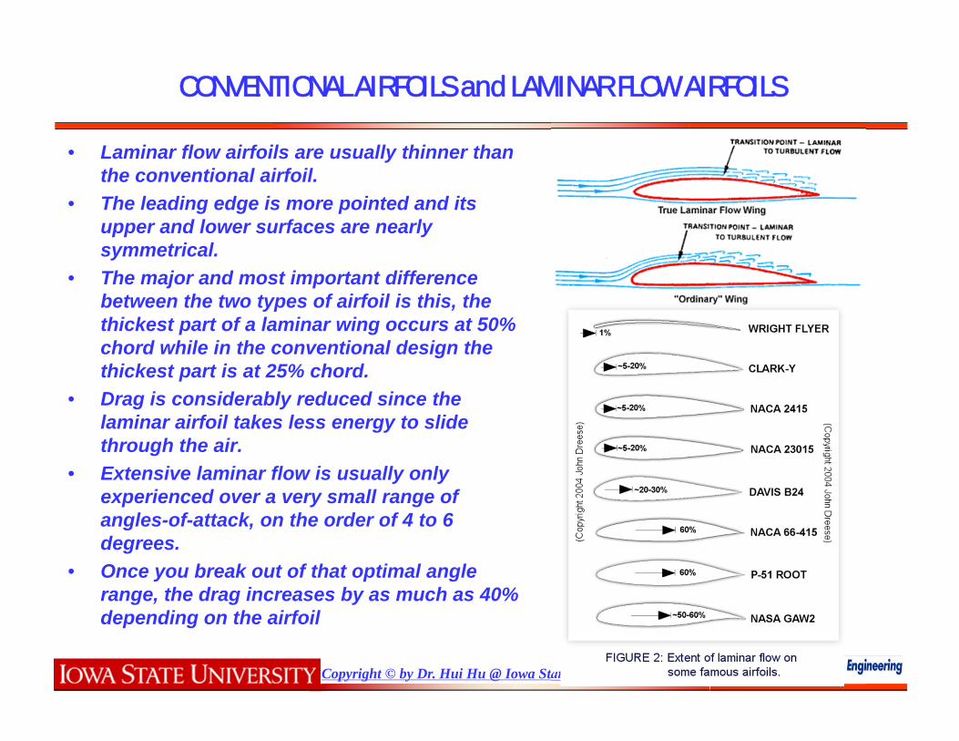
CONVENTIONAL AIRFOILS and LAMINAR FLOW AIRFOILS

• Laminar flow airfoils are usually thinner than the conventional airfoil.

• The leading edge is more pointed and its upper and lower surfaces are nearly symmetrical.

• The major and most important difference between the two types of airfoil is this, the thickest part of a laminar wing occurs at 50% chord while in the conventional design the thickest part is at 25% chord.

• Drag is considerably reduced since the laminar airfoil takes less energy to slide through the air.

• Extensive laminar flow is usually only experienced over a very small range of angles-of-attack, on the order of 4 to 6 degrees.

• Once you break out of that optimal angle range, the drag increases by as much as 40% depending on the airfoil


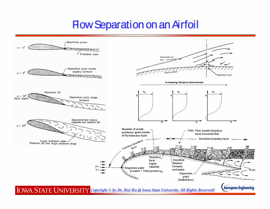
Flow Separation on an Airfoil


Aerodynamic Performance of An Airfoil

X/C *100

Y/C

*100

-20 0 20 40 60 80 100 120

-40

-20

0

20

40

60

vort: -4.5 -3.5 -2.5 -1.5 -0.5 0.5 1.5 2.5 3.5 4.5

shadow region

GA(W)-1 airfoil

25 m/s

0.2

0.4

0.6

0.8

1.0

1.2

1.4

0 2 4 6 8 10 12 14 16 18 20

CL=2Experimental data

Angle of Attack (degrees)

Lift

Coe

ffici

ent,

Cl

0

0.05

0.10

0.15

0.20

0.25

0.30

0.35

0.40

0 2 4 6 8 10 12 14 16 18 20

Experimental data

Angle of Attack (degrees)

Dra

g C

oeffi

cien

t, C

d

X/C *100

Y/C

*100

-40 -20 0 20 40 60 80 100 120 140

-60

-40

-20

0

20

40

60

vort: -4.5 -3.5 -2.5 -1.5 -0.5 0.5 1.5 2.5 3.5 4.5

shadow region

GA(W)-1 airfoil

25 m/s

Airfoil stall

Airfoil stall

Before stall

After stallcV

DCd2

21

cV

LCl2

21


Flow Separation and Transition on Low-Reynolds-number Airfoils

• Low-Reynolds-number airfoil (with Re<500,000) aerodynamics is important for both military and civilian applications, such as propellers, sailplanes, ultra-light man-carrying/man-powered aircraft, high-altitude vehicles, wind turbines, unmanned aerial vehicles (UAVs) and Micro-Air-Vehicles (MAVs).

• Since laminar boundary layers are unable towithstand any significant adverse pressure gradient, laminar flow separation is usually found on low-Reynolds-number airfoils. Post-separation behavior of the laminar boundary layers would affect the aerodynamic performances of the low-Reynolds-number airfoils significantly

• Separation bubbles are usually found to formon the upper surfaces of low-Reynolds-number airfoils . Separation bubble would burstsuddenly to cause airfoil stall at high AOA when the adverse pressure gradient becoming too big.


-0.10-0.05

00.050.100.15

0 0.1 0.2 0.3 0.4 0.5 0.6 0.7 0.8 0.9 1.0

X/C

Y/C

-3 .0

-2 .5

-2 .0

-1 .5

-1 .0

-0 .5

0

0 .5

1 .0

1 .50 0 .1 0 .2 0 .3 0 .4 0 .5 0 .6 0 .7 0 .8 0 .9 1 .0

A O A = 06 degA O A = 08 degA O A = 09 degA O A = 10 degA O A = 11 degA O A = 12 degA O A = 14 deg

X / CC

P

Separation point

Turbulence transition

Reattachment point

Surface Pressure Coefficient distributions (Re=68,000)

Typical surface pressure distribution when a laminar separation bubble is formed (Russell, 1979)

7 .5

8 .0

8 .5

9 .0

9 .5

1 0 .0

1 0 .5

1 1 .0

1 1 .5

1 2 .0

0 0 .0 5 0 .10 0 .1 5 0 .20 0 .2 5 0 .30 0 .3 5 0 .40 0 .4 5 0 .50

T ra n s itio n R e a tta ch m e n tS e p a ra tio n

X /C

AO

A (d

egre

e)

GA (W)-1 airfoil(also labeled as NASA LS(1)-0417 )


Laminar Separation Bubble on a Low-Reynolds-number Airfoil

PIV measurement results at AOA = 10 deg, Re=68,000

X/C*100

Y/C

*100

-5 0 5 10 15 20 25 30 35

0

5

10

-18.0 -14.0 -10.0 -6.0 -2.0 2.0 6.0 10.0 14.0 18.0

10 m/sGA (W)-1 airfoilSpawisevorticity

X/C*100

Y/C

*100

-5 0 5 10 15 20 25 30 35

0

5

10

U m/s: 2.0 4.0 6.0 8.0 10.0 12.0 14.0 16.0 18.0

GA (W)-1 airfoilreattachmentseparation

X/C*100

Y/C

*100

18 20 22 24 26 28 30 32 343

4

5

6

7

8

9

10

11

U m/s: 2.00 4.00 6.00 8.00 10.00 12.00 14.00 16.00 18.00

10 m/sReattachment

X/C*100

Y/C

*100

18 20 22 24 26 28 30 32 343

4

5

6

7

8

9

10

11

-25.0 -20.0 -15.0 -10.0 -5.0 0.0 5.0 10.0 15.0 20.0 25.0

SpanwiseVorticity(1/s * 103)

10 m/s

Instantaneous flow field Ensemble-averaged flow field

(Hu et al., ASME Journal of Fluid Engineering, 2008)


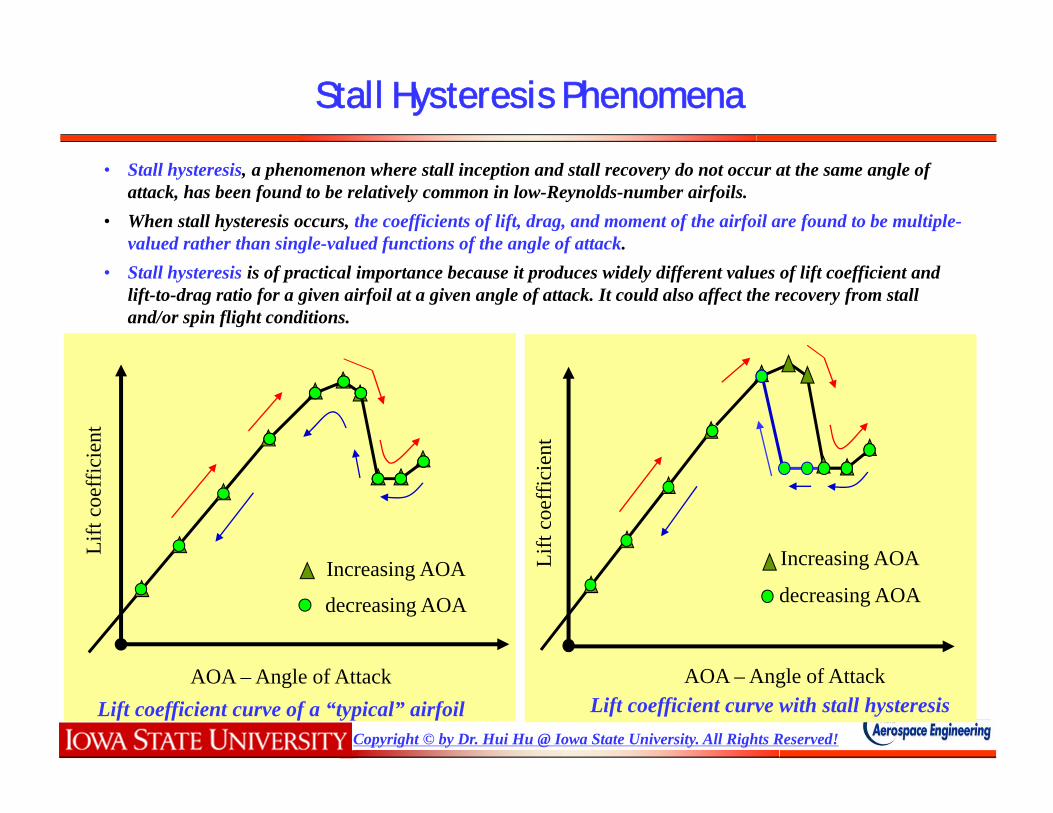
Stall Hysteresis Phenomena

• Stall hysteresis, a phenomenon where stall inception and stall recovery do not occur at the same angle of attack, has been found to be relatively common in low-Reynolds-number airfoils.

• When stall hysteresis occurs, the coefficients of lift, drag, and moment of the airfoil are found to be multiple-valued rather than single-valued functions of the angle of attack.

• Stall hysteresis is of practical importance because it produces widely different values of lift coefficient and lift-to-drag ratio for a given airfoil at a given angle of attack. It could also affect the recovery from stall and/or spin flight conditions.

Increasing AOA

decreasing AOA

AOA – Angle of Attack

Lift

coef

ficie

nt

Lift coefficient curve of a “typical” airfoil Lift coefficient curve with stall hysteresisAOA – Angle of Attack

Increasing AOA

decreasing AOA

Lift

coef

ficie

nt


Measured airfoil lift and drag coefficient profiles

-0.2

0

0.2

0.4

0.6

0.8

1.0

1.2

1.4

1.6

-4 -2 0 2 4 6 8 10 12 14 16 18 20

AOA increasingAOA decreasing

Angle of Attack (degree)

Lift

Coe

ffici

ent,

Cl

Hysteresis loop

0

0.05

0.10

0.15

0.20

0.25

0.30

0.35

0.40

-4 -2 0 2 4 6 8 10 12 14 16 18 20

AOA increasingAOA decreasing


Dra

g C

oeffi

cien

t, C

d

Hysteresisloop

• The hysteresis loop was found to be clockwise in the lift coefficient profiles, and counter-clockwise in the drag coefficient profiles.

• The aerodynamic hysteresis resulted in significant variations of lift coefficient, Cl, and lift-to-drag ratio, l/d,for the airfoil at a given angle of attack.

• The lift coefficient and lift-to-drag ratio at AOA = 14.0 degrees were found to be Cl = 1.33 and l/d = 23.5when the angle is at the increasing angle branch of the hysteresis loop.

• The values were found to become Cl = 0.8 and l/d = 3.66 for the same AOA=14.0 degrees when the angle is at the deceasing angle branch of the hysteresis loop

GA(W)-1 airfoil, ReC = 160,000


0.5

0.6

0.7

0.8

0.9

1.0

1.1

1.2

1.3

1.4

1.5

8 9 10 11 12 13 14 15 16 17 18 19 20

AOA decreasing

AOA increasing


Lift

Coe

ffici

ent,

Cl

PIV Measurement results

X/C *100

Y/C

*100

-40 -20 0 20 40 60 80 100 120 140

-60

-40

-20

0

20

40

60

vort: -4.5 -3.5 -2.5 -1.5 -0.5 0.5 1.5 2.5 3.5 4.5

shadow region

GA(W)-1 airfoil

25 m/s

X/C *100

Y/C

*100

-20 0 20 40 60 80 100 120

-40

-20

0

20

40

60

vort: -4.5 -3.5 -2.5 -1.5 -0.5 0.5 1.5 2.5 3.5 4.5

shadow region

GA(W)-1 airfoil

25 m/s

X/C *100

Y/C

*100

-20 0 20 40 60 80 100 120

-40

-20

0

20

40

60

vort: -4.5 -3.5 -2.5 -1.5 -0.5 0.5 1.5 2.5 3.5 4.5

shadow region

GA(W)-1 airfoil

25 m/s

separation bubble

X/C *100

Y/C

*100

-40 -20 0 20 40 60 80 100 120 140

-60

-40

-20

0

20

40

vort: -4.5 -3.5 -2.5 -1.5 -0.5 0.5 1.5 2.5 3.5 4.5

shadow region

GA(W)-1 airfoil

25 m/s

(Hu, Yang, Igarashi, Journal of Aircraft, Vol. 44. No. 6 , 2007)


0.5

0.6

0.7

0.8

0.9

1.0

1.1

1.2

1.3

1.4

1.5

8 9 10 11 12 13 14 15 16 17 18 19 20

AOA decreasing

AOA increasing


Lift

Coe

ffici

ent,

Cl

Refined PIV Measurement Results

X/C *100

Y/C

*100

-5 0 5 10 15 20 25 30 35-10

-5

0

5

10

15

20

25

-18.0 -14.0 -10.0 -6.0 -2.0 2.0 6.0

GA(W)-1 airfoil 25 m/s

X/C *100

Y/C

*100

-5 0 5 10 15 20 25 30 35-10

-5

0

5

10

15

20

25

vort: -18.0 -14.0 -10.0 -6.0 -2.0 2.0 6.0

GA(W)-1 airfoil 25 m/s

X/C *100

Y/C

*100

-5 0 5 10 15 20 25 30 35

-5

0

5

10

15

20

vort: -18.0 -14.0 -10.0 -6.0 -2.0 2.0 6.0

GA(W)-1 airfoil25 m/s

X/C *100

Y/C

*100

-5 0 5 10 15 20 25 30 35

-10

-5

0

5

10

15

20

vort: -18.0 -14.0 -10.0 -6.0 -2.0 2.0 6.0

GA(W)-1 airfoil25 m/s

(Hu, Yang, Igarashi, Journal of Aircraft, Vol. 44. No. 6 , 2007)


y

x

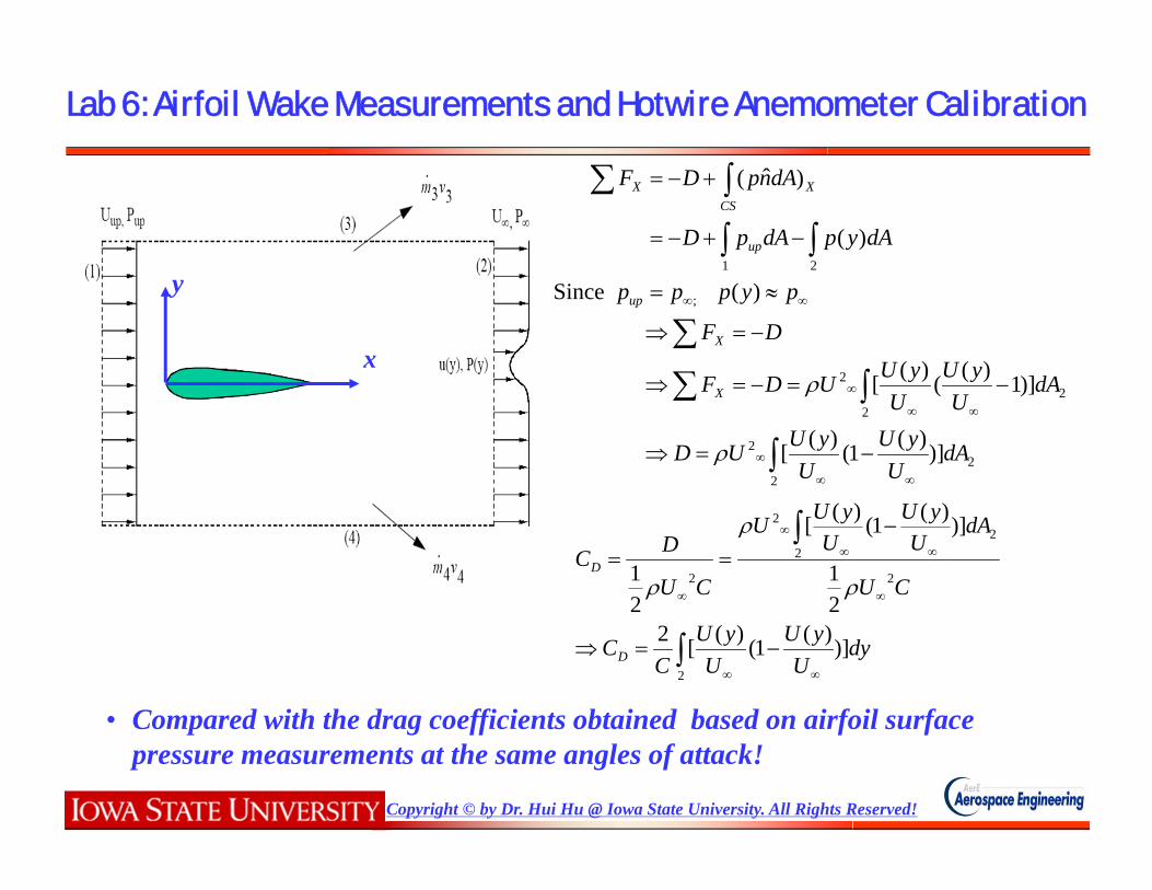
Lab 6: Airfoil Wake Measurements and Hotwire Anemometer Calibration

22

2

22

2

;

21

)])(1()([

)]1)(()([

)( Since

)(

)ˆ(

dAU

yUU

yUUD

dAU

yUU

yUUDF

DF

pyppp

dAypdApD

dAnpDF

X

X

up

up

CSXX

2

2

22

2

2

)])(1()([221

)])(1()([

21

dyU

yUU

yUC

C

CU

dAU

yUU

yUU

CU

DC

D

D

• Compared with the drag coefficients obtained based on airfoil surface pressure measurements at the same angles of attack!


y

x80 mm

Pressure rake with 41 total pressure probes(the distance between the probes d=2mm)




CTA hotwire probe

Flow Field

Current flow through wire

V

),(2ww

w TVqRidt

dTmc

• Constant-temperature anemometry


Hotwire Anemometer Calibration

0

2

4

6

8

10

12

14

16

18

20

1.0 1.1 1.2 1.3 1.4 1.5 1.6 1.7 1.8 1.9 2.0 2.1 2.2

Curve fittingExperimental data

y=a+bx+cx2+d*x3+e*x4 max dev:0.166, r2=1.00a=10.8, b=3.77, c=-26.6, d=13.2

voltage (V)

Flow

vel

ocity

(m/s

)

• To quantify the relationship between the flow velocity and voltage output from the CTA probe


Required Measurement Results

Required Plots:

• Cp distribution in the wake (for each angle of attack) for the airfoil wake measurements

• Cd vs angle of attack (do your values look reasonable?) based on the airfoil wake

measurements

• Your hot wire anemometer calibration curve: Velocity versus voltage output of hotwire

anemometer (including a 4th order polynomial fit)

Please briefly describe the following details:

• How you calculated your drag—you should show your drag calculations

• How these drag calculations compared with the drag calculations you made in the previous

experiment.

• Reynolds number of tests and the incoming flow velocity

lecture # 07: laminar and turbulent flowshuhui/teaching/2014sx/class-notes/aere344... ·...

Documents