lecture 1 - computer science · · 2005-06-30specral graph theory and its applications september...

Specral Graph Theory and its Applications September 2, 2004

Lecture 1

Lecturer: Daniel A. Spielman

1.1 A quick introduction

First of all, please call me “Dan”. If such informality makes you uncomfortable, you can try“Professor Dan”. Failing that, I will also answer to “Prof. Spielman”.

As the title suggests, this course is about the eigenvalues and eigenvectors of matrices associatedwith graphs, and their applications. To be honest, I should say that we will occasionally considerthe spectra of matrices that do not come from graphs. But, our approach to these matrices willbe sufficiently combinatorial that it will be a lot like looking at graphs. In this lecture, I hope tosurvey much of the material that we will cover in the course. You will see that I have way too muchmaterial in mind to cover in one course. So, we will pare down the list of topics as the semesterprogresses.

1.2 Matrices for Graphs

First, we recall that a graph G = (V,E) is specified by its vertex set, V , and edge set E. In anundirected graph, the edge set is a set of unordered pairs of vertices. Unless otherwise specified,all graphs will be undirected, and finite.

Without loss of generality, we may assume that V = {1, . . . , n}. The most natural matrix toassociate with G is its adjacency matrix, AG, whose entries ai,j are given by

ai,j =

{

1 if (i, j) ∈ E

0 otherwise.

I usually prefer to consider the Laplacian matrix of a graph, LG, whose entries li,j are given by

li,j =

−1 if (i, j) ∈ E

di if i = j, and

0 otherwise,

where di is the degree of vertex i.

It is probably not obvious that the eigenvalues or eigenvectors of AG or LG should tell you anythinguseful about the graph G. However, they say a lot! In fact, whenever I meet a strange graph, thefirst thing I do is examine its eigenvectors and eigenvalues.

1-1

Lecture 1: September 2, 2004 1-2

Let’s quickly compute the spectra of LG for a simple graph G. In this case, we’ll take V = {1, 2, 3}and E = {(1, 2), (2, 3)}:

1 2 3

Figure 1.1: The path graph on 3 vertices

We first observe that the vector (1, 1, 1) is an eigenvector of eigenvalue 0. We’ll just compute thevalue we get at the second node when we multiply this vector by LG. First, we get 2 times thevalue that was there, 1. We then subtract off the value at each of its neighbors, also 1. Thus, weget 0.

1 2 3

1 11

*2 *1*1

*(−1)*(−1)

Figure 1.2: The all 1s vector is an eigenvector with eigenvalue 0.

In the figure below, we display the other eigenvectors above the graph, and the vector you get bymultiplying by LG below.

1 2 3

1 2 3

−1 0 1

1

3 3

−1 0 1

−2

−6

1

Figure 1.3: The other eigenvectors: (−1, 0, 1) and (1,−2, 1).

In fact, for every Laplacian the all 1s vector is an eigenvector of eigenvalue 0, and all other eigen-values are non-negative. We’ll prove that next class. You might want to think of your own proofbefore then.

Perhaps the most important thing to take from this example is that an eigenvector is a functionon the vertices. That is, it assigns a real number to each vertex.

1.3 Spectral Embeddings

As we just said, an eigenvector assigns a real number to each vertex. So, if we take two eigenvectors,then we obtain two real numbers for each vertex. This suggests a way of drawing a graph: taketwo eigenvectors, v and w, and plot vertex i at the point v(i), w(i). If we take v and w to be theeigenvectors corresponding to the two smallest non-zero eigenvalues of the Laplacian, this oftengives us a very good picture of a graph. Let’s look at some examples.


Rather than give you the graph by a list of edges, I’ll give you a drawing of it. In the figure, eachline segment in the picture is an edge, and each point at which edges meet is a vertex. Clearly, thisis a planar graph.

load yale

gplot(A,p)

50 100 150 200 250 300 3500

50

100

150

200

250

300

In the following figure, we draw the graph using the eigenvectors of the two smallest non-zeroeigenvalues of the Laplacian matrix of the graph as the x and y coordinates.

gplot(A,x(:,2:3))

−0.1 −0.08 −0.06 −0.04 −0.02 0 0.02 0.04 0.06 0.08 0.1−0.1

−0.08

−0.06

−0.04

−0.02

0

0.02

0.04

0.06

0.08

0.1

This picture should convince you that the eigenvectors say a lot about a graph! In particular, fornice planar graphs, they provide a good set of coordinates for the vertices.

Let’s do some more examples. Just to show you that these pictures aren’t always ideal, let’s takeout the book in the center of the shield (and slightly modify the graph).


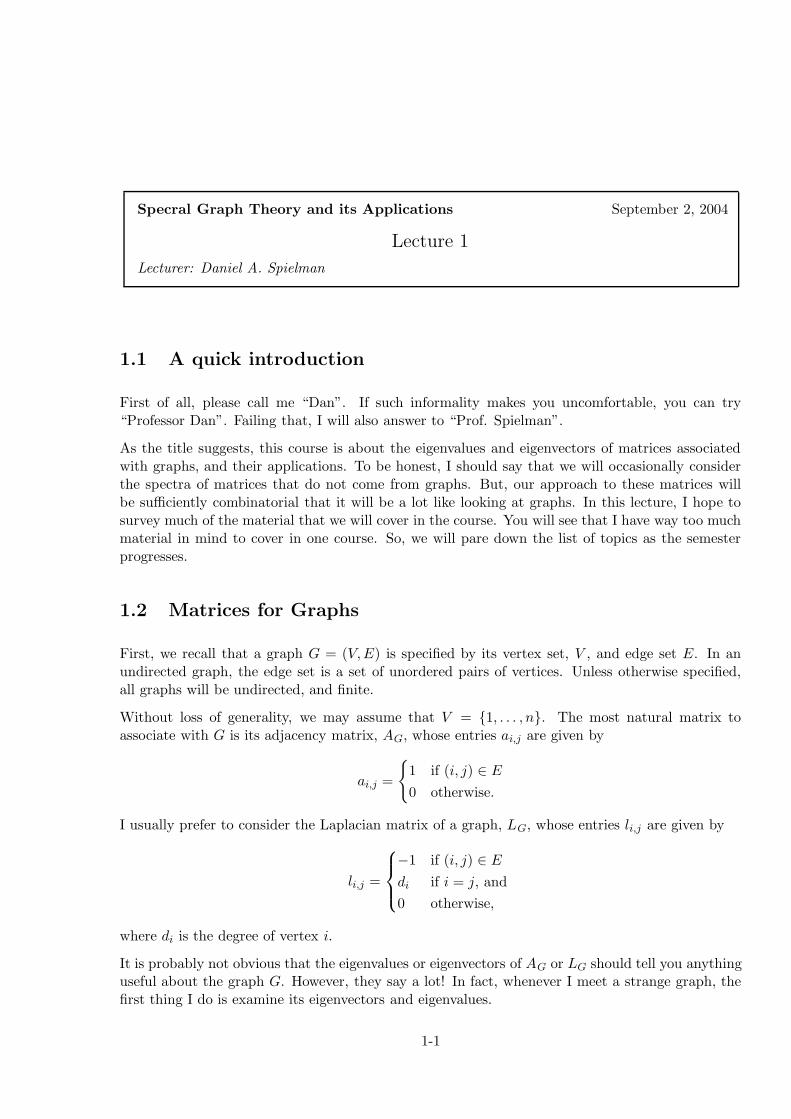
load yale2

gplot(A,p)

50 100 150 200 250 300 3500

50

100

150

200

250

300

And now, we’ll give its spectral embedding.

gplot(A,x(:,2:3))

−0.08 −0.06 −0.04 −0.02 0 0.02 0.04 0.06 0.08−0.08

−0.06

−0.04

−0.02

0

0.02

0.04

0.06

0.08

That figure wasn’t quite as nice. But, let’s zoom in on a little part on the right.

0.064 0.066 0.068 0.07 0.072 0.074

−0.025

−0.02

−0.015

−0.01

−0.005

0

0.005

0.01

0.015

0.02

Here’s the famous airfoil graph.


load airfoil1

gplot(A,xy)

−0.2 0 0.2 0.4 0.6 0.8 1 1.2 1.4−0.8

−0.6

−0.4

−0.2

0

0.2

0.4

0.6

0.8

And, here’s its spectral embedding.

gplot(A,v(:,1:2))

−0.04 −0.03 −0.02 −0.01 0 0.01 0.02−0.02

−0.015

−0.01

−0.005

0

0.005

0.01

0.015

0.02

0.025

0.03

Finally, let’s look at a spectral embedding of the edges of the dodecahedron.

load dodec.txt

E = dodec;

A = sparse(E(:,1),E(:,2),1);

A = A + A’;

L = diag(sum(A)) - A;

[v,d] = eig(full(L));

gplot(A,v(:,2:3))

−0.4 −0.3 −0.2 −0.1 0 0.1 0.2 0.3 0.4−0.4

−0.3

−0.2

−0.1

0

0.1

0.2

0.3

0.4


You will notice that this looks like what you would get if you squashed the dodecahedron downto the plane. The reason is that we really shouldn’t be drawing this picture in two dimensions:the smallest non-zero eigenvalue of the Laplacian has multiplicity three. So, we can’t reasonablychoose just two eigenvectors. We should be choosing three that span the eigenspace. If we do, wewould get the canonical representation of the dodecahedron in three dimensions.

1.3.1 Why?

You might wonder why the eigenvectors supply such good pictures of nice planar graphs. I don’tthink that anyone has proven a satisfactory theorem about this. But, I do have some intution. Fornow, I will just mention the intution that comes from a theorem of Tutte. It says that if you takea three-connected planar graph, select any face, fix the positions of the vertices of that face at thecorners of a polygon, and then fix every other vertex to be the center of gravity of its neighbors,then you get a straight-line planar embedding. Alternatively, you can think of every edge as arubber band. We then nail down the vertices on the outside face, and let all the others go wherethey will. If the graph is planar and three-connected, then this is a planar embedding.

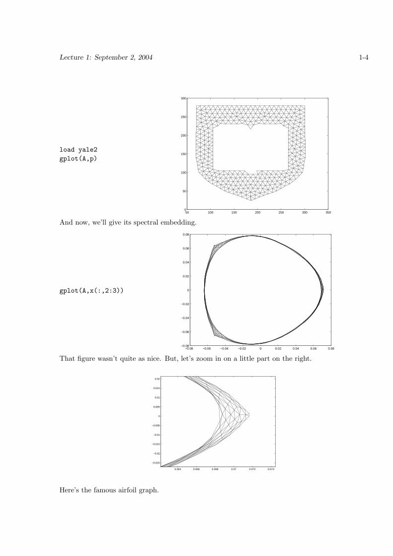
Algebraically, we compute this embedding by solving a linear system in the Laplacian.

Here’s an example of what happens when we do this for the dodecahedron.

l2 = L;

l2(1:5,:) = 0;

l2(1:5,1:5) = eye(5);

phi = 2*pi*[0:4]/5;

b = [[cos(phi)’,sin(phi)’];

zeros(15,2)];

x = l2 / b;

gplot(A,x)

−1 −0.8 −0.6 −0.4 −0.2 0 0.2 0.4 0.6 0.8 1−1

−0.8

−0.6

−0.4

−0.2

0

0.2

0.4

0.6

0.8

1

Of course, in the spectral case there is no distinguished outside face, so this isn’t exactly what isgoing on.

I’d be interested in trying to prove something about these embeddings, and would be happy to talkabout the problem.


1.3.2 Other eigenvectors

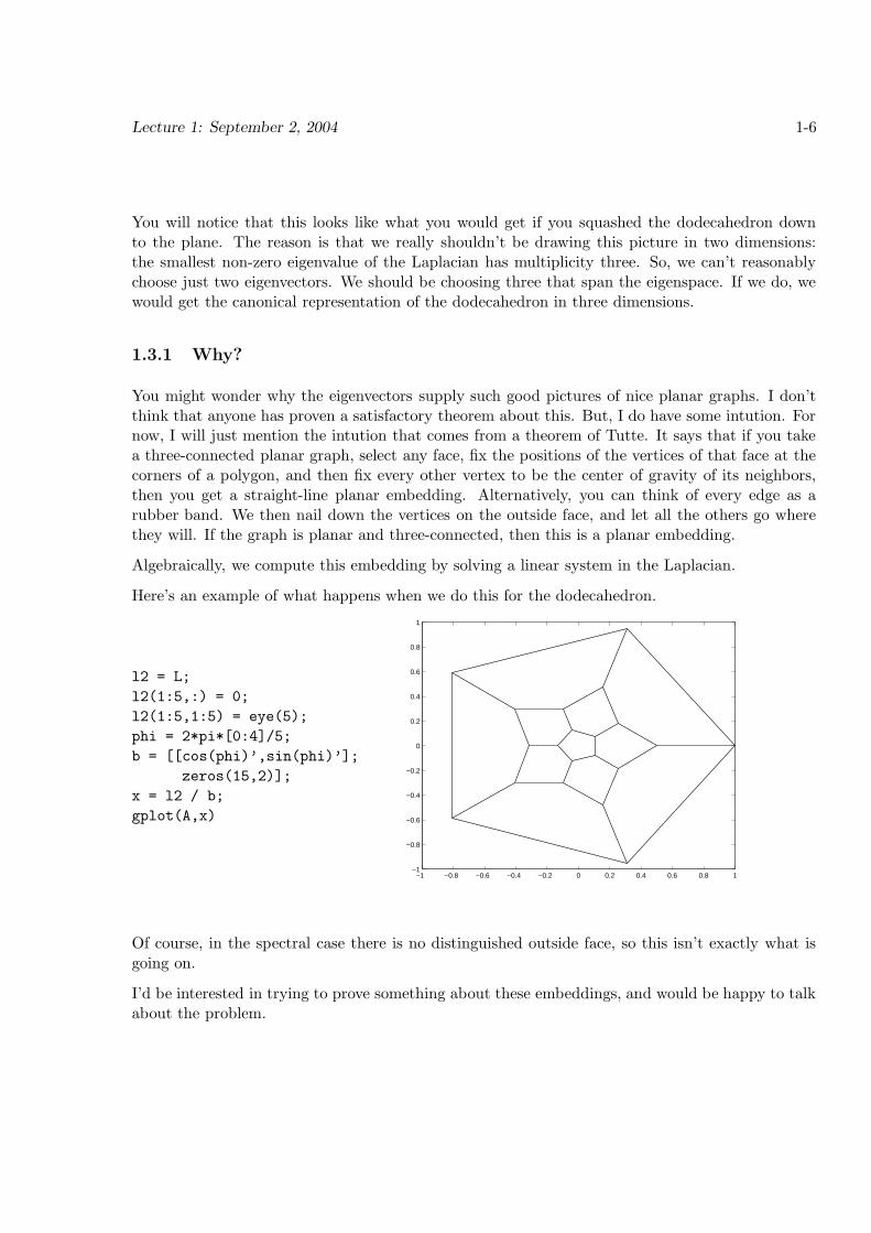
What if we chose to draw using other eigenvectors? For example, we could use the eigenvectors oflargest eigenvalue. In the case of the dodecahedron, we get the following embedding from the 19thand 20th eigenvectors:

gplot(A,v(:,19:20))

−0.4 −0.3 −0.2 −0.1 0 0.1 0.2 0.3 0.4−0.4

−0.3

−0.2

−0.1

0

0.1

0.2

0.3

0.4

In this image, each vertex is far from its neighbors. This suggests that we might be able to usethese eigenvectors for coloring. I recall that the problem of graph coloring is that of assigning acolor to each vertex so that each edge connects vertices of different colors. The goal is to use asfew colors as possible. While we can’t always use these eigenvectors for coloring, they do provide avery good heuristic. We might prove later in the semester that they work well on random graphschosen so that they have colorings with few colors.

1.4 Isomorphism

One of the oldest problems in graph theory is that of determining whether or not two graphs areisomorphic. Two graphs G = (V,E) and H = (V, F ) are isomorphic if there is a permutationπ : V → V such that (i, j) ∈ E if and only if (π(i), π(j)) ∈ F . That is, π is a way of re-labeling thevertices that makes the two graphs the same.

Determining the complexity of graph isomorphism is a maddening task. For every pair of graphsI have ever seen, it has been easy to tell whether or not they are isomorphic. However, the bestbound on the worst-case complexity for the problem is 2O(

√

n).

From the examples above, one would suspect that eigenvectors and eigenvalues would be very helpfulin determining whether or not two graphs are isomorphic. For example, if we let λ1 ≤ λ2 ≤ · · · ≤ λn

be the eigenvalues of LG and µ1 ≤ µ2 ≤ · · ·µn be the eigenvalues of LH , then λi 6= µi implies thatG and H are non-isomorphic.

Exercise Prove this! Also prove that G and H are isomorphic if and only if there exists apermutation matrix P such that AH = PAGP T .


However, this does not determine graph isomorphism because there are non-isomorphic graphs withthe same spectra.

But, we can also use the eigenvectors to help test for isomorphism. For example, the spectralembeddings above were uniquely determined up to a rotation. One can prove (and you will)

Exercise Let λ1 ≤ · · · ≤ λn be the eigenvalues of AG. Assume that λi is isolated, that isλi−1 < λi < λi+1 and let vi be the corresponding eigenvector. Let H be a graph isomorphicto G, and let wi be the ith eigenvector of G. Then, there exists a permutation π such thatvi(j) = wi(π(j)).

So, if we can find a few eigenvectors that map each vertex to a distinct point, then we can use themto test for isomorphism.

Unfortuntely, there exist graphs for which the eigenvectors do not tell us very much.

The following graph has an eigenvector that only has two values.

load gcube;

[v,d] = eig(full(m));

v(:,1)

ans =

-0.2500

-0.2500

0.2500

0.2500

0.2500

0.2500

-0.2500

-0.2500

0.2500

0.2500

-0.2500

-0.2500

-0.2500

-0.2500

0.2500

0.2500

However, this is not fatal. As we will see during the course, if every eigenvector has multiplicityless than m, then it is possible to test isomorphism in time nm+O(1).

However, there exist graphs in which there are no non-trivial eigenvalues of small multiplicity.

load lsg;


[v,d] = eig (full (A));

diag (d)

ans =

-3.0000

-3.0000

-3.0000

-3.0000

-3.0000

-3.0000

-3.0000

-3.0000

-3.0000

-3.0000

-3.0000

-3.0000

2.0000

2.0000

2.0000

2.0000

2.0000

2.0000

2.0000

2.0000

2.0000

2.0000

2.0000

2.0000

12.0000

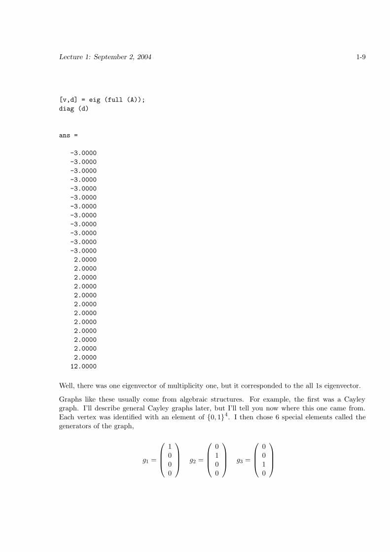
Well, there was one eigenvector of multiplicity one, but it corresponded to the all 1s eigenvector.

Graphs like these usually come from algebraic structures. For example, the first was a Cayleygraph. I’ll describe general Cayley graphs later, but I’ll tell you now where this one came from.Each vertex was identified with an element of {0, 1}4. I then chose 6 special elements called thegenerators of the graph,

g1 =

1000

g2 =

0100

g3 =

0010


g4 =

0001

g5 =

1100

g6 =

1010

I then created an edge (x, x + gi) for each x ∈ {0, 1}4 and 1 ≤ i ≤ 6.

Cayley graphs are generalizations of this construction, in which we replace {0, 1}4 with any groupand require that the generator set be closed under inversion. The eigenvectors and eigenvalues ofCayley graphs are closely related to their irreducible representations. When the group is abelian,the eigenvectors do not depend on the choice of generator set.

The second graph was a strongly-regular graph. These are a maddening family of graphs in whichthe eigenvectors essentially provide no help in determining isomorphism.

Algebraic constructions of graphs provide the power behind many algorithms and constructions inthe theory of computing and error-correcting codes. We will see many of them.

1.5 Random Graphs

There are two fancy ways to construct graphs: by algebraic constructions and at random. It turnsout that random graphs are almost as nice as algebraic graphs, and are sometimes nicer. If theyare large enough, random graphs should really be thought of as a special family of graphs. We willsee that the spectra of random graphs are very well behaved.

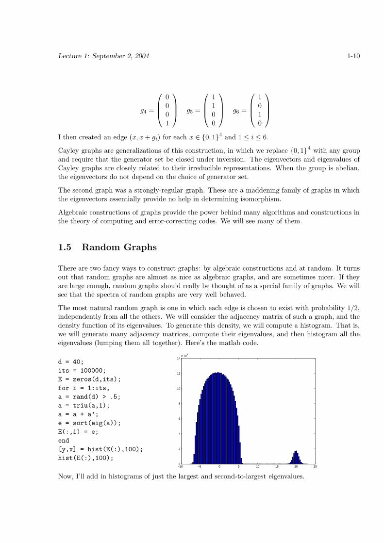
The most natural random graph is one in which each edge is chosen to exist with probability 1/2,independently from all the others. We will consider the adjacency matrix of such a graph, and thedensity function of its eigenvalues. To generate this density, we will compute a histogram. That is,we will generate many adjacency matrices, compute their eigenvalues, and then histogram all theeigenvalues (lumping them all together). Here’s the matlab code.

d = 40;

its = 100000;

E = zeros(d,its);

for i = 1:its,

a = rand(d) > .5;

a = triu(a,1);

a = a + a’;

e = sort(eig(a));

E(:,i) = e;

end

[y,x] = hist(E(:),100);

hist(E(:),100);−10 −5 0 5 10 15 20 250

2

4

6

8

10

12

14x 10

4

Now, I’ll add in histograms of just the largest and second-to-largest eigenvalues.


[y1,x1] = hist(E(40,:),100);

sc = x(2) - x(1);

sc1 = x1(2) - x1(1);

hold on

plot(x1,y1 *sc / sc1, ’r’,...

’LineWidth’,5)

[y2,x2] = hist(E(39,:),100);

sc2 = x2(2) - x2(1);

plot(x2,y2 *sc / sc2, ’g’,...

’LineWidth’,5)

−10 −5 0 5 10 15 20 250

2

4

6

8

10

12

14x 10

4

Note that these distributions are very tightly concentrated. Almost everything that we are seeinghere can be proved analytically. This includes the form of the big hump in the limit.

x1 = x / sqrt(d);

s1 = sqrt(1-x1.^2);

z = s1 / s1(23) * y(23);

plot(x-1/2,z,’c’,’LineWidth’,5)

−10 −5 0 5 10 15 20 250

2

4

6

8

10

12

14x 10

4

1.6 The Spectral Gap

We now get to my favorite eigenvalue, λ2 of the Laplacian. That is, the smallest non-zero eigenvalue.It is often called the Fiedler value. Whenever I see a graph, the first thing that I want to knowabout it is its Fiedler value. In particular, it helps me distinguish many families of graphs. Hereare some sample values


Graph Fiedler Value

Path Θ(1/n2)Grid Θ(1/n)

3d grid Θ(n−2/3)Expander Θ(1)binary tree Θ(1/n)dumbell Θ(1/n)

By a dumbell, I mean two expanders joined by one edge. If you don’t yet know what an expanderis, don’t worry. You will.

One of the reasons the Fiedler value is exciting is that it tells you how well you can cut a graph. Acut of a graph is a division of its vertices into two sets, S and S̄. We usually want to find cuts thatcut as few edges as possible. We let E(S, S̄) denote the set of edges whose vertices lie on oppositesides of the cut. We then define the ratio of the cut to be

φ(S) =

∣

∣E(S, S̄)∣

∣

min(|S| ,∣

∣S̄∣

∣).

The best cut is the one of minimum ratio, and its quality is the isoperimetric number of a graph

φ(G) = minS

φ(S).

A version of Cheeger’s inequality says that the isoperimetric number is intimately related to λ2.

Theorem 1.6.1.

φ ≥ λ2 ≥ φ2

2d,

where d is an upper bound the the degree of every vertex in the graph.

If we appropriately scale the isoperimetric number and the Laplacian, it is possible to get rid ofthe d in the inequality.

By Cheeger’s inequality, λ2 says something good about every graph. If λ2 is small, then it ispossible to cut the graph into two pieces without cutting too many edges. If λ2 is large, then everycut of the graph must cut many edges. Expanders are graphs in which λ2 is large, where largemight mean Θ(1) or very close to d. I could teach a whole course on expanders, and some have.The short story is that good constructions of expanders exist, and they enable good constructionsof all sort of other things, from error-correcting codes to pseudo-random generators.

Here’s another useful property of expanders.

Theorem 1.6.2. Let G = (V,E) be a d-regular connected graph on n nodes such that d − λ2 < µ.

Then, for every S, T ⊆ V with |S| = αn and |T | = βn, we have

|E(S, T ) − dαβn| ≤ µn√

(α − α2)(β − β2).


That is, if µ is small, then for every pair of sets of vertices S and T , the number of edges betweenS and T is close to what you would expect to find if you chose S and T at random. There areexplicit constructions of expanders in which µ

∑

2√

d − 1.

Using λ2, we can also answer questions such as: “how much does a random subgraph of G look likeG”?

1.7 Quantum Computing

1.8 Graph approximation and preconditioning

What does it mean for one graph to approximate another? Here is one definition.

Definition 1.8.1. A graph G is a c-approximation of H if for all x ∈ Rn,

xT LGx ≤ xT LHx ≤ xT LGx.

In the class, we will see how to prove the following two theorems.

Theorem 1.8.2. For every weighted graph G, there exists a weighted graph H with at most

n logO(1) n edges that (1 + ε) approximates G.

Theorem 1.8.3. For every weighted graph G, there exists a weighted graph H with at most n +t logO(1) n edges that n/t approximates G.

We will see that these results can be used to quickly solve diagonally-dominant linear systems.

1.9 Summary

I see three ways of looking at spectral graph theory: descriptive, algorithmic, and controlling. In thedescriptive world, we determine what we can learn about a graph from its spectra. In the algorithmicframework, we use this descriptive knowledge to design algorithms. In the controlling framework,we design graphs whose eigenvalues meet certain restrictions. If believe that by improving ourdescriptive understanding, we can improve efforts at control.

1.10 Mechanics

This course is designed for graduate students. While there is no book for the course, I will supplyreference material for each lecture. Sometimes this will be a paper, and often it will be my lecturenotes.

The work load should not be too high. There will be two problem sets, and each student will scribeone lecture. If there are few enough students, then each may give a presentation at the end of thesemester.

lecture 1 - computer science · · 2005-06-30specral graph theory and its applications september...

Documents