Lecture 1: Single processor performance

Why parallel computing

• Solving an 𝑛 × 𝑛 linear system Ax=b by using Gaussian

elimination takes ≈ 1

3𝑛3 flops.

• On Core i7 975 @ 4.0 GHz, which is capable of about 60-70 Gigaflops

𝑛 flops time

1000 3.3×108 0.006 seconds

1000000 3.3×1017 57.9 days

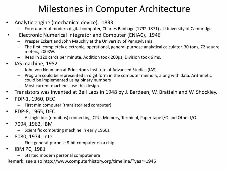
Milestones in Computer Architecture • Analytic engine (mechanical device), 1833

– Forerunner of modern digital computer, Charles Babbage (1792-1871) at University of Cambridge

• Electronic Numerical Integrator and Computer (ENIAC), 1946 – Presper Eckert and John Mauchly at the University of Pennsylvania – The first, completely electronic, operational, general-purpose analytical calculator. 30 tons, 72 square

meters, 200KW. – Read in 120 cards per minute, Addition took 200µs, Division took 6 ms.

• IAS machine, 1952 – John von Neumann at Princeton’s Institute of Advanced Studies (IAS) – Program could be represented in digit form in the computer memory, along with data. Arithmetic

could be implemented using binary numbers – Most current machines use this design

• Transistors was invented at Bell Labs in 1948 by J. Bardeen, W. Brattain and W. Shockley. • PDP-1, 1960, DEC

– First minicomputer (transistorized computer)

• PDP-8, 1965, DEC – A single bus (omnibus) connecting CPU, Memory, Terminal, Paper tape I/O and Other I/O.

• 7094, 1962, IBM – Scientific computing machine in early 1960s.

• 8080, 1974, Intel – First general-purpose 8-bit computer on a chip

• IBM PC, 1981 – Started modern personal computer era

Remark: see also http://www.computerhistory.org/timeline/?year=1946

www.top500.org

Over 17 years, 10000-fold increases.

Motherboard diagram of PC

http://en.wikipedia.org/wiki/Front-side_bus

http://education-portal.com/academy/lesson/what-is-a-motherboard-definition-function-diagram.html#lesson

Intel S2600GZ4 Server Motherboard

• CPU Type: Dual Intel Xeon E5-2600 Series • Maximum Memory Supported: 768GB • Intel® C600 Chipset http://www.memoryexpress.com/

Motherboard diagram of S2600GZ4

http://www.intel.com/content/www/us/en/chipsets/server-chipsets/server-chipset-c600.html

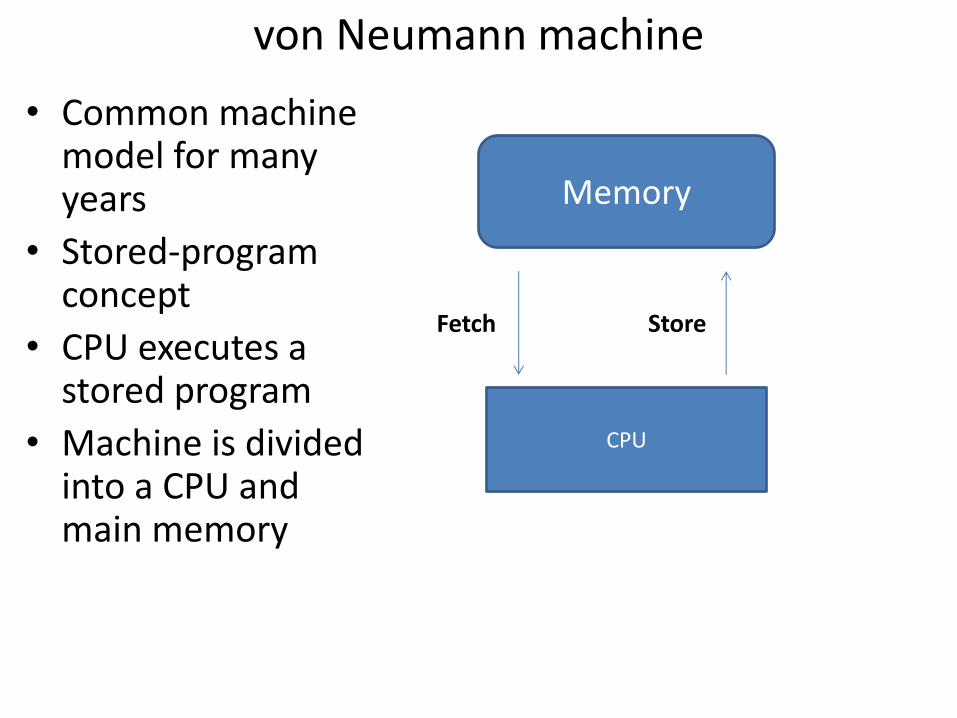
von Neumann machine

• Common machine model for many years

• Stored-program concept

• CPU executes a stored program

• Machine is divided into a CPU and main memory

Memory

CPU

Fetch Store

Machine Language, Assembly and C

• CPU understands machine language only • Assembly language is easier to understand:

– Abstraction – A unique translation (every CPU has a different set of assembly

instructions) Remark: Nowadays we use Assembly only when:

1. Processing time is critical and we need optimize the execution 2. Low level operations, such as operating on registers etc. are needed, but not

supported by the high level language. 3. Memory is critical, and optimizing its management is required.

• C language: – The translation is not unique. It depends on Compiler and optimization. – It is portable.

program

High-level language program

Compiler Assembler Linker Computer

Assembly language program

Structured Machines

Problem-oriented language level

Assembly language level

Operating system machine level

Instruction set architecture level (ISA)

Microarchitecture level

Digital logic level

Translation (compiler)

Translation (assembler)

Partial interpretation (operating system)

Interpretation (microprogram) or direct execution

Hardware

Swap (int v[], int k) { int temp; temp = v[k]; v[k] = v[k+1]; v[k+1] = temp; }

High-level language program (in C)

Assembly language program (for microprocessor without interlocked pipeline stages (MIPS), which is an instruction set architecture (ISA))

lw $15, 0($2) //load word at RAM address ($2+0) into register $15

lw $16, 4($2) sw $16, 0($2) // store word in register $16 into RAM at address ($2+0)

sw $15, 4($2)

Binary machine language program (for MIPS)

0000 1001 1100 0110 1010 1111 0101 1000

1010 1111 0101 1000 0000 1001 1100 0110

1100 0110 1010 1111 0101 1000 0000 1001

0101 1000 0000 1001 1100 0110 1010 1111

Execution Cycle

Instruction

Fetch

Instruction

Decode

Operand

Fetch

Execute

Result

Store

Next

Instruction

Obtain instruction from program storage

Determine required actions and instruction size

Locate and obtain operand data

Compute result value or status

Deposit results in storage for later use

Determine successor instruction

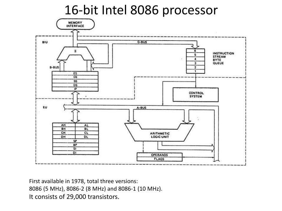
16-bit Intel 8086 processor

First available in 1978, total three versions: 8086 (5 MHz), 8086-2 (8 MHz) and 8086-1 (10 MHz).

It consists of 29,000 transistors.

• 8086 CPU is divided into two independent functional units:

1. Bus Interface Unit (BIU)

2. Execution Unit (EU)

• The 8086 is internally a 16-bit CPU and externally it has a 16-bit data bus. It has the ability to address up to 1 Mbyte of memory via its 20-bit address bus.

Control Unit: • Generate control/timing signals • Controls decoding/execution of instructions

Registers (very fast memories): • General-Purpose Registers (AX, BX, CX, DX): holds temporary results or addresses

during execution of instructions. results of ALU operations. Write results to memory

• Instruction Pointer Counter: Holds address of instruction being executed • Segment registers (CS, DS, SS, ES): combine with others to generate memory

address to reference 1Mb memory • Instruction register: holds instruction while it’s decoded/executed

Arithmetic Logic Unit (ALU): ALU takes one or two operands A,B Operation:

1. Addition, Subtraction (integer) 2. Multiplication, Division (integer) 3. And, Or, Not (logical operation) 4. Bitwise operation (shifts, equivalent to multiplication by power of 2)

Specialized ALUs: • Floating Point Unit (FPU) • Address ALU

Memory read transaction (1)

• Load content of address A into register eax

• CPU places address A on the system bus, I/O bridge passes it onto the memory bus

Load operation: movl A, %eax Remark: here we use GNU Assembly language

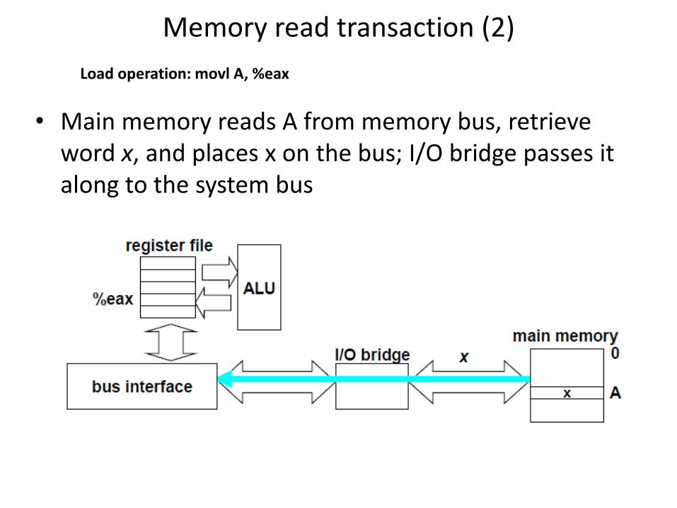
Memory read transaction (2)

• Main memory reads A from memory bus, retrieve word x, and places x on the bus; I/O bridge passes it along to the system bus

Load operation: movl A, %eax

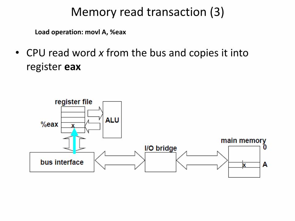
Memory read transaction (3)

• CPU read word x from the bus and copies it into register eax

Load operation: movl A, %eax

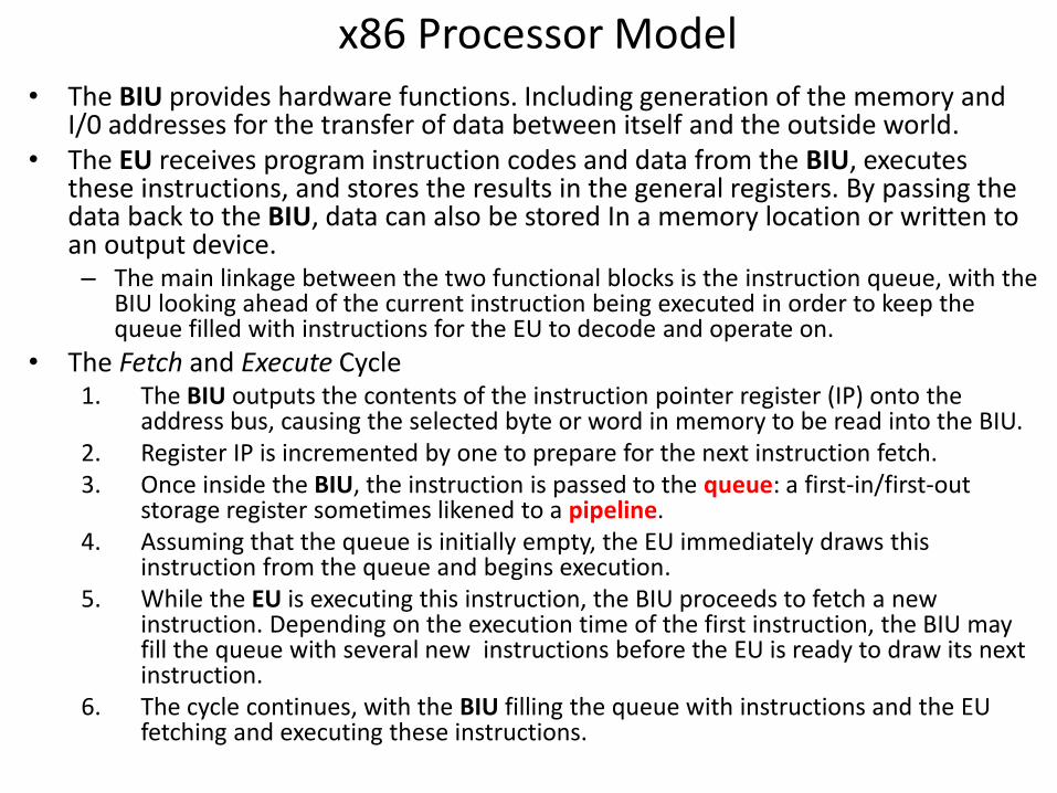
x86 Processor Model • The BIU provides hardware functions. Including generation of the memory and

I/0 addresses for the transfer of data between itself and the outside world. • The EU receives program instruction codes and data from the BIU, executes

these instructions, and stores the results in the general registers. By passing the data back to the BIU, data can also be stored In a memory location or written to an output device. – The main linkage between the two functional blocks is the instruction queue, with the

BIU looking ahead of the current instruction being executed in order to keep the queue filled with instructions for the EU to decode and operate on.

• The Fetch and Execute Cycle 1. The BIU outputs the contents of the instruction pointer register (IP) onto the

address bus, causing the selected byte or word in memory to be read into the BIU. 2. Register IP is incremented by one to prepare for the next instruction fetch. 3. Once inside the BIU, the instruction is passed to the queue: a first-in/first-out

storage register sometimes likened to a pipeline. 4. Assuming that the queue is initially empty, the EU immediately draws this

instruction from the queue and begins execution. 5. While the EU is executing this instruction, the BIU proceeds to fetch a new

instruction. Depending on the execution time of the first instruction, the BIU may fill the queue with several new instructions before the EU is ready to draw its next instruction.

6. The cycle continues, with the BIU filling the queue with instructions and the EU fetching and executing these instructions.

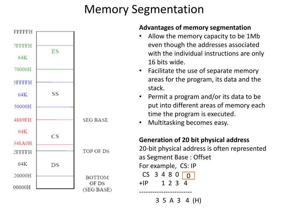
Memory Segmentation

Advantages of memory segmentation • Allow the memory capacity to be 1Mb

even though the addresses associated with the individual instructions are only 16 bits wide.

• Facilitate the use of separate memory areas for the program, its data and the stack.

• Permit a program and/or its data to be put into different areas of memory each time the program is executed.

• Multitasking becomes easy. Generation of 20 bit physical address 20-bit physical address is often represented as Segment Base : Offset For example, CS: IP CS 3 4 8 0 +IP 1 2 3 4 ------------------------ 3 5 A 3 4 (H)

0

Moore’s law • Gordon Moore’s observation in 1965: the number of

transistors per square inch on integrated circuits had doubled every year since the integrated circuit was invented (often interpreted as Computer performance doubles every two years (same cost))

(Gordon_Moore_ISSCC_021003.pdf)

Moore’s law

• Moore’s revised observation in 1975: the pace slowed down a bit, but data density had doubled approximately every 18 months

• Moore’s law is dead

Gordon Moore quote from 2005: “in terms of size [of transistor] ..we’re approaching the size of atoms which is a fundamental barrier...”

Date Intel Transistors CPU (x1000)

Technology

1971 4004 2.3

1978 8086 31 2.0 micron

1982 80286 110 HMOS

1985 80386 280 0.8 micron CMOS

1989 80486 1200

1993 Pentium 3100 0.8 micron biCMOS

1995 Pentium Pro 5500 0.6 micron – 0.25

Implicit Parallelism - Pipelining

• Super instruction pipeline – more stages – 20 stage pipeline in Pentium 4

• Example: 𝑆1 = 𝑠2 + 𝑆3; – Stages gone through: 1. Unpack operands; 2. Compare

exponents; 3. Align significant digits; 4. Add fractions; 5. Normalize fraction; 6. Pack operands.

– Assembly instructions load R1, @S2

load R2, @S3

add R1, R2 // (6 stages)

store R1, @S1

– 9 clock cycles to complete one operation

• Register numbers begin with the letter r, like r0, r1, r2.

• Immediate (scalar) values begin with the hash mark #, like #100, #200.

• Memory addresses begin with the at sign @, like @1000, @1004.

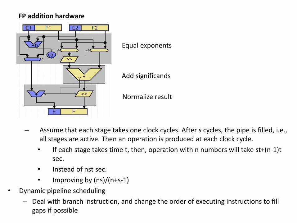
Equal exponents

Add significands

Normalize result

FP addition hardware

– Assume that each stage takes one clock cycles. After s cycles, the pipe is filled, i.e., all stages are active. Then an operation is produced at each clock cycle.

• If each stage takes time t, then, operation with n numbers will take st+(n-1)t sec.

• Instead of nst sec.

• Improving by (ns)/(n+s-1)

• Dynamic pipeline scheduling

– Deal with branch instruction, and change the order of executing instructions to fill gaps if possible

Implicit Parallelism - Superscalar execution

• Superscalar – performing instructions in parallel

– Performing two instructions simultaneously, which means to fetch two instructions together, decode them at the same time, execute, i.e..

• Example Superscalar execution Consider a processor (or a virtual machine) with two pipelines and the ability to simultaneously issue two instructions. These processors are sometimes also referred to as super-pipelined processors. The ability of a processor to issue multiple instructions in the same cycle is referred to as superscalar execution. • Register numbers begin

with the letter r, like r0, r1, r2.

• Immediate (scalar) values begin with the hash mark #, like #100, #200.

• Memory addresses begin with the at sign @, like @1000, @1004.

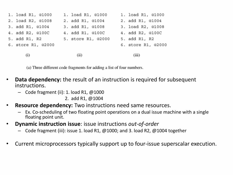
• Data dependency: the result of an instruction is required for subsequent instructions. – Code fragment (ii): 1. load R1, @1000 2. add R1, @1004

• Resource dependency: Two instructions need same resources. – Ex. Co-scheduling of two floating point operations on a dual issue machine with a single

floating point unit.

• Dynamic instruction issue: issue instructions out-of-order – Code fragment (iii): issue 1. load R1, @1000; and 3. load R2, @1004 together

• Current microprocessors typically support up to four-issue superscalar execution.

Effect of memory latency on performance (1) von Neumann Bottleneck: the transfer of data and instructions between memory and the CPU is inherently sequential.

• Latency of the memory: the time that a CPU takes to get a block of data from the memory system.

• Bandwidth of the memory: the rate at which data can be pumped from the memory to the processor.

Effect of memory latency on performance (2)

Example. Assume a CPU operates at 1GHz (1 ns clock) and is connected to a DRAM with a latency of 100 ns. Assume the CPU has 2 multiply-add units and is capable of executing 4 instructions in each cycle of 1 ns. The peak CPU rating is 4GFLOPS (floating-point operations per second).

Since the memory latency is 100 cycles, CPU must wait 100 cycles before it can process data. Therefore, the peak speed of computation is 10MFLOPS.

Remark: 10MFLOPS/4GFLOPS = 1/400.

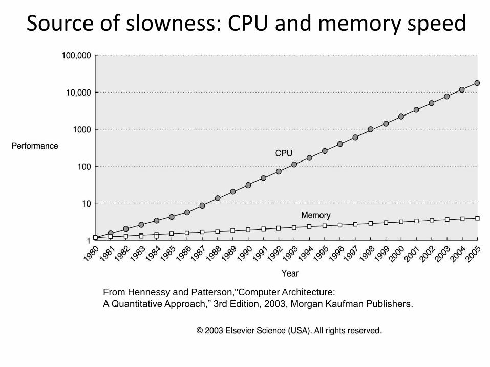
Source of slowness: CPU and memory speed

From Hennessy and Patterson,"Computer Architecture:

A Quantitative Approach,” 3rd Edition, 2003, Morgan Kaufman Publishers.

Improving effective memory latency using cache memories (1)

• Put a look-up table of recently used data onto the CPU chip. • Cache memories are small, fast SRAM-based memories

(low memory latency) managed automatically in hardware. • CPU look first for data in L1, then in L2,…, then in main

memory

Hierarchy of increasingly bigger, slower memories

Organization of a cache memory

Core i7 cache hierarchies

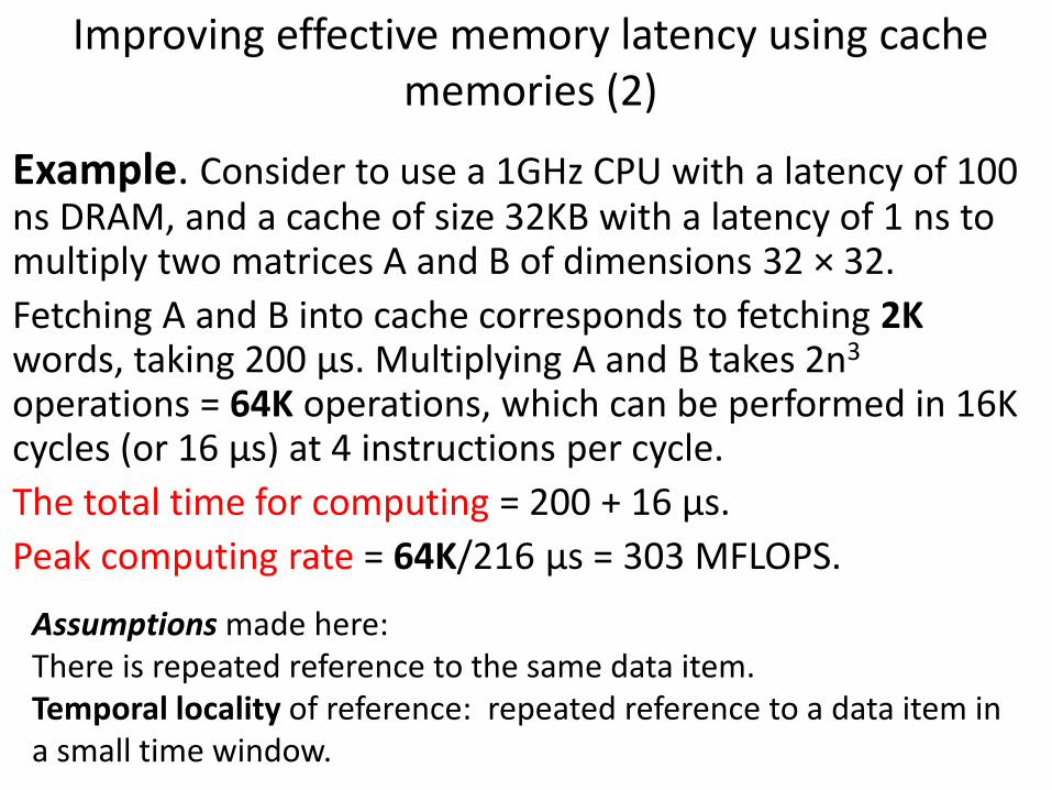
Improving effective memory latency using cache memories (2)

Example. Consider to use a 1GHz CPU with a latency of 100 ns DRAM, and a cache of size 32KB with a latency of 1 ns to multiply two matrices A and B of dimensions 32 × 32.

Fetching A and B into cache corresponds to fetching 2K words, taking 200 μs. Multiplying A and B takes 2n3 operations = 64K operations, which can be performed in 16K cycles (or 16 μs) at 4 instructions per cycle.

The total time for computing = 200 + 16 μs.

Peak computing rate = 64K/216 μs = 303 MFLOPS.

Assumptions made here: There is repeated reference to the same data item. Temporal locality of reference: repeated reference to a data item in a small time window.

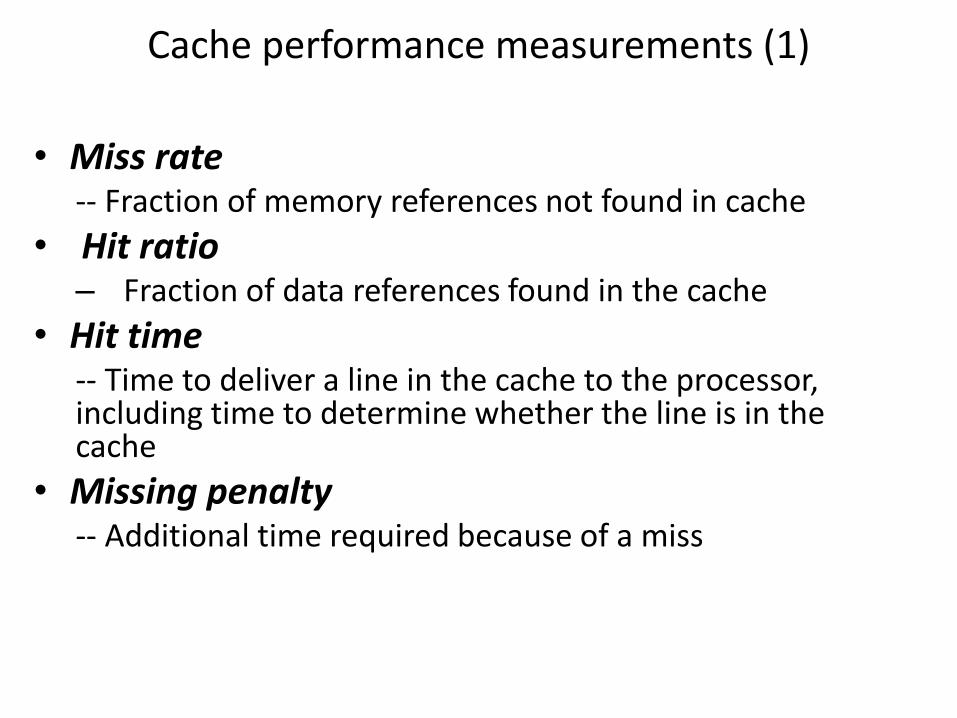
Cache performance measurements (1)

• Miss rate -- Fraction of memory references not found in cache

• Hit ratio – Fraction of data references found in the cache

• Hit time -- Time to deliver a line in the cache to the processor, including time to determine whether the line is in the cache

• Missing penalty -- Additional time required because of a miss

Cache performance measurements (2)

• Big difference between a hit and a miss

Example. Assume that cache hit time is 1 cycle, and miss penalty is 100 cycles. A 99% hit rate is twice as good as 97% rate.

-- Average access time

1. 97% hit rate: 0.97* 1 + 0.03*(1+100) = 4 cycles

2. 99% hit rate: 0.99*1 + 0.01*(1+100) = 2 cycles

Remark: The effective computation rate of many applications is bounded not by the processing rate of the CPU, but by the rate at which data can be pumped into the CPU.

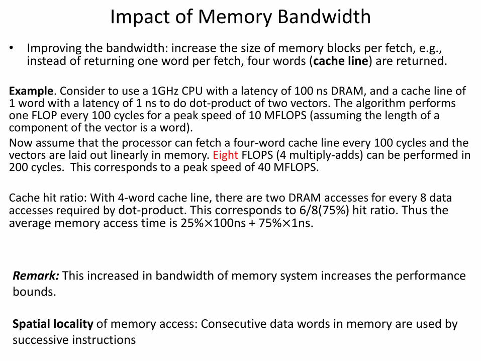
• Improving the bandwidth: increase the size of memory blocks per fetch, e.g., instead of returning one word per fetch, four words (cache line) are returned.

Example. Consider to use a 1GHz CPU with a latency of 100 ns DRAM, and a cache line of 1 word with a latency of 1 ns to do dot-product of two vectors. The algorithm performs one FLOP every 100 cycles for a peak speed of 10 MFLOPS (assuming the length of a component of the vector is a word). Now assume that the processor can fetch a four-word cache line every 100 cycles and the vectors are laid out linearly in memory. Eight FLOPS (4 multiply-adds) can be performed in 200 cycles. This corresponds to a peak speed of 40 MFLOPS. Cache hit ratio: With 4-word cache line, there are two DRAM accesses for every 8 data accesses required by dot-product. This corresponds to 6/8(75%) hit ratio. Thus the average memory access time is 25%×100ns + 75%×1ns.

Impact of Memory Bandwidth

Remark: This increased in bandwidth of memory system increases the performance bounds. Spatial locality of memory access: Consecutive data words in memory are used by successive instructions

Writing cache-friendly code (1)

• Principle of locality: -- programs tend to reuse/use data items recently used or nearby those recently used -- Temporal locality: Recently referenced items are likely to be referenced in the near future -- Spatial locality: Items with nearby addresses tend to be referenced close together in time

Data -- Reference array elements in succession: spatial locality -- Reference “sum” in each iteration: temporal locality

Instructions -- Reference instructions in sequence: Spatial locality -- Cycle through loop repeatedly: Temporal locality

How caches take advantage of temporal locality

• The first time the CPU reads from an address in main memory, a copy of that data is also stored in the cache.

-- The next time that same address is read, the copy of the data in the cache is used instead of accessing the slower DRAM

• Commonly accessed data is stored in the faster cache memory

How caches take advantage of spatial locality

• When the CPU reads location i from main memory, a copy of that data is placed in the cache.

• Instead of just copying the contents of location i, we can copy several values into the cache at once, such as the four words from locations i through i+3.

– If the CPU does need to read from locations i+1, i+2 or i+3, it can access that data from the cache.

Writing cache-friendly code (2)

In C/C++ language, array is stored in row-major order in memory

Assume that there is a 4-words cache with 4-words cache lines. Left code has miss rate = ¼ = 25% Right code has miss rate = 100% Remark: programming with better spatial locality

• Example: Compute column sums of a matrix 1. for(i = 0; i < 1024; i++){ 2. c_sum[i]= 0.0; 3. for(j = 0; j<1024; j++) 4. c_sum[i] += b[j][i]; 5. }

• Problems associated with this code: – Poor cache utilization (frequent cache misses). The j loop

accesses entries in b[][]. This corresponds to accessing every 1024-th entry in the 1D array of b[0][0], b[0][1],…,b[0][1023], b[1][0],….

– No spatial locality. It’s likely that one word per cache line fetched from memory will be used.

• Swapping loop order:

1. for(i = 0; i < 1024; i++)

2. c_sum[i]= 0.0;

3. for(j = 0; j < 1024; j++){

4. for(i = 0; i<1024; i++)

5. c_sum[i] += b[j][i];

6. }

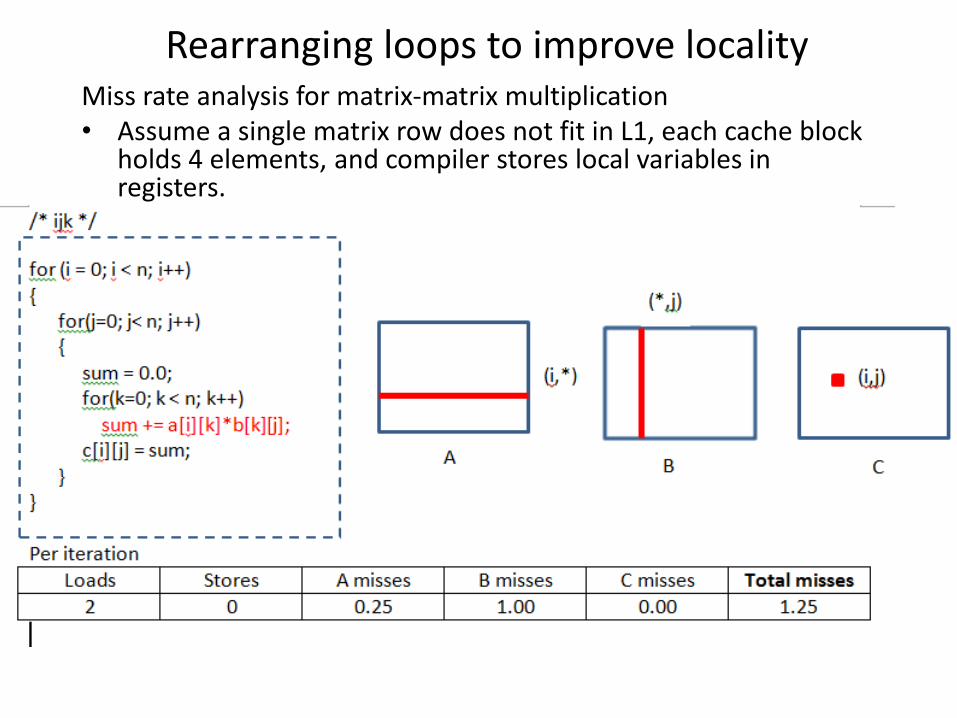
Rearranging loops to improve locality Miss rate analysis for matrix-matrix multiplication • Assume a single matrix row does not fit in L1, each cache block

holds 4 elements, and compiler stores local variables in registers.

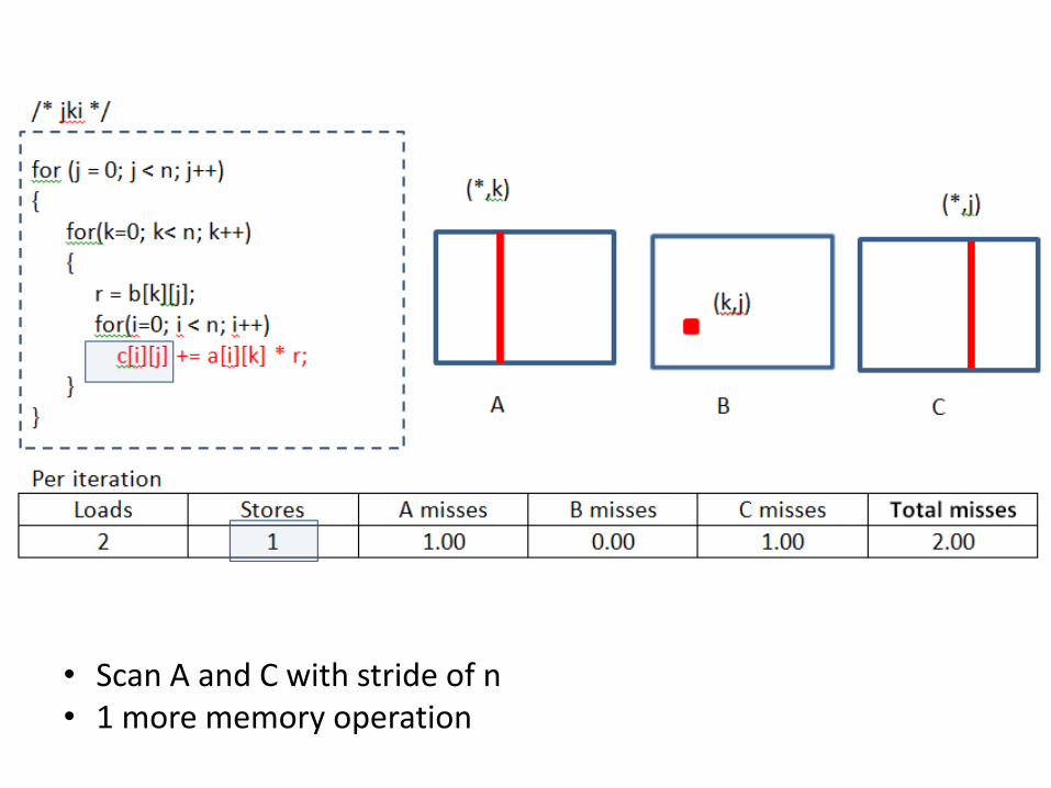
• Scan A and C with stride of n • 1 more memory operation

Trade-off: one memory operation – fewer misses

Core i7 Matrix-matrix multiplication performance

From EECS213 Northwestern University

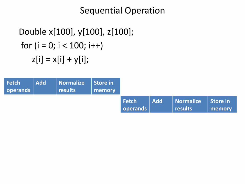
Sequential Operation

Double x[100], y[100], z[100];

for (i = 0; i < 100; i++)

z[i] = x[i] + y[i];

Fetch operands

Add Normalize results

Store in memory

Fetch operands

Add Normalize results

Store in memory

Solution: Pipelining

Divide a computation into stages that can support concurrency.

Double x[100], y[100], z[100];

for (i = 0; i < 100; i++)

z[i] = x[i] + y[i];

Fetch operands

Add Normalize results

Store in memory

Fetch operands

Add Normalize results

Store in memory

Fetch operands

Add Normalize results

Store in memory

Fetch operands

Add Normalize results

Store in memory

time

Another improvement: Vector processor pipeline. Example: Cray 90

Loop unrolling:

for (i = 0; i < 100; i++)

do_a(i);

for (i = 0; i < 50; i+=2) { do_a(i); do_a(i+1); } Remark: Loop unrolling can reduce the number of loop maintenance instruction executions by the loop unrolling factor

Example: for (i = 0; i < 1000; i++) { a[i] = b[i] + c[i]; }

for (i = 0; i < 1000; i+=2) { a[i] = b[i] + c[i]; a[i+1] = b[i+1] + c[i+1]; }

Loop Unrolling

Software Pipelining Software pipeline the C loop: for (i=1000;i>=1;i--)

x[i]=x[i]+s;

t=x[1000]; g=t+s; t=x[999]; for (i=1000;i>=2;i--) { x[i]=g; // i store g=t+s; // i-1 add t=x[i-2]; // i-2 load } x[2]=g; g=t+s; x[1]=g;

Load x[i]

Incr x[i] Load x[i-1]

Store x[i] Incr x[i-1] Load x[i-2]

Store x[i-1] Incr x[i-2] Load x[i-3]

time