lecture 1: what is matlab? - power...

1/31/2015

1

Lecture 1: What is MATLAB?

Dr. Mohammed HawaElectrical Engineering Department

University of Jordan

EE201: Computer Applications. See Textbook Chapter 1.

Copyright © Dr. Mohammed Hawa Electrical Engineering Department, University of Jordan

MATLAB

• MATLAB (MATrix LABoratory) is a numerical computing environment and programming language.

• Developed by MathWorks.• MATLAB is widely used to solve engineering and

science problems in academic and research institutions as well as the industry.

• In MATLAB, problems are expressed in familiar mathematical notation.

• MATLAB is an interactive system whose basic data element is a matrix (remember C/C++ arrays!).

• Open-source alternative is: GNU Octave.• Paid alternative: LabVIEW MathScript

2

1/31/2015

2


MATLAB can be used for:

• Matrix manipulations (math computations).• Data analysis, exploration, and plotting.• Implementation of algorithms.• Creation of user interfaces.• Data acquisition.• Interfacing with programs written in other

languages, (e.g., C, C++, Java, and Fortran).• An optional toolbox (with MuPAD symbolic

engine) allows accessing symbolic computing.• An additional package, Simulink®, adds graphical

simulation and model-based design.

3


Like a VERY advanced calculator

Would you go to an engineering exam without a calculator?

4

1/31/2015

3


Solving Simultaneous Equations

• Find the values of xand y that satisfy the following equations simultaneously :

• Can be solved by hand to get:x = 1, y = 2

• Remember how?

5


Simultaneous Equations

• Solving simultaneous equations:

• Can be solved by hand to get:

x = 1.2, y = 2.8, z = 0.6

• How?

6

1/31/2015

4


Solving Simultaneous Equations

• Many variables:

• Humans are note good at this. MATLAB (a computer software) is!

7


MATLAB solution

8

1/31/2015

5


MATLAB is powerful!

• We often need to solve systems with 10,000 or 100,000 simultaneous equations (could be non-linear or differential equations too)

• Can be done very quickly using a computer

• This is common in engineering– Electrical circuits

– Image recognition

– Communication systems (MIMO, OFDM, etc)

– Operations research

– Mechanics and dynamics, etc

9


MATLAB vs. Programming languages

• MATLAB is a vector-based numerical analysis language:– Can be used as an advanced calculator and

graphing tool– Also can be used as a programming language

• This is different than the programming languages you are familiar with (C, C++, …)– Can be a little frustrating since it takes time and

effort to write code in MATLAB– But the code is very effective and can be refined

gradually

10

1/31/2015

6


Know about MATLAB

• MATLAB is easy to begin with but needs hard work to master.

• MATLAB is optimized for performing matrix operations.• MATLAB is interpreted

– for the most part slower than a compiled language such as C++– but interactive and simplifies fixing errors

• Although primarily procedural, MATLAB does have some object-oriented elements.

• MATLAB is NOT a general purpose programming language• MATLAB is designed for scientific computation and is not

suitable for some things (such as parsing text)• MATLAB is very useful for data analysis and rapid

prototyping, but is not designed for large-scale system development.

11


Let us run MATLAB …

12

1/31/2015

7


MATLAB Environment

13


MATLAB as a Calculator

• You can enter expressions at the command line and evaluate them right away.

• The >> symbols indicate where commands are typed.

14

1/31/2015

8


Mathematical Operators

15


Order of Precedence (BEDMAS)

• B = Brackets• E = Exponentials• D = Division• M = Multiplication• A = Addition• S = Subtraction

• Careful using brackets: check that opening and closing brackets are matched up correctly.

16

1/31/2015

9


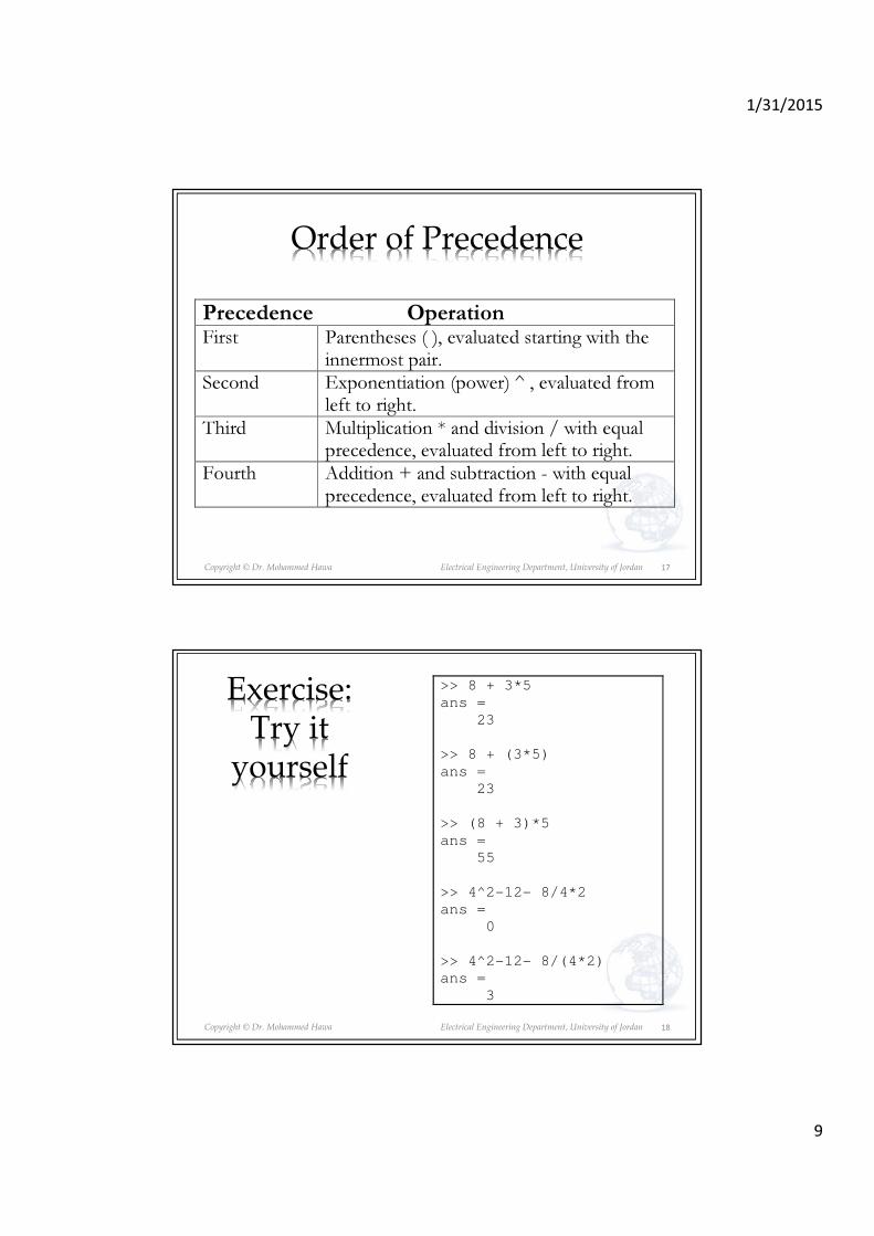
Order of Precedence

Precedence Operation First Parentheses ( ), evaluated starting with the

innermost pair. Second Exponentiation (power) ^ , evaluated from

left to right. Third Multiplication * and division / with equal

precedence, evaluated from left to right. Fourth Addition + and subtraction - with equal

precedence, evaluated from left to right.

17


Exercise:Try it

yourself

>> 8 + 3*5

ans =

23

>> 8 + (3*5)

ans =

23

>> (8 + 3)*5

ans =

55

>> 4^2-12- 8/4*2

ans =

0

>> 4^2-12- 8/(4*2)

ans =

3

18

1/31/2015

10


Entering Commands

• MATLAB retains your previous keystrokes.• Use the ↑ key to scroll back through previous

commands.• Press the ↑ key once to see the previous entry, and

so on.• Use the ↓ key to scroll forward. • Edit a line using the ← and → arrow keys, the

Backspace key, and the Delete key.• Press the Enter key to execute the command.• You can copy (highlight & ctrl+c) from Command

History window to the Command Window.

19


Built-in Math Constants

pi �: ratio of circle's circumference to its diameter

i √−1: Imaginary unit

j √−1: Imaginary unit

Inf ∞: Infinity

NaN Not-a-Number

intmax Largest value of integer type

intmin Smallest value of integer type

ans Temporary variable containing the most recent answer

eps The accuracy of floating point precision

…

>> 2*pi

ans =

6.2832

>> Inf+100000

ans =

Inf

>> format long g

>> 2*pi

ans =

6.28318530717959

>> 1+ans

ans =

7.28318530717959

20

1/31/2015

11


Exercise>> 1/0

ans =

???

>> 0/0

ans =

???

>> 7/2*i

ans =

???

>> 7/2i

ans =

???

21


Exercise: Answers>> 1/0

ans =

Inf

>> 0/0

ans =

NaN

>> 7/2*i

ans =

0 + 3.5000i

>> 7/2i

ans =

0 - 3.5000i

22

1/31/2015

12


Possible Formats

23


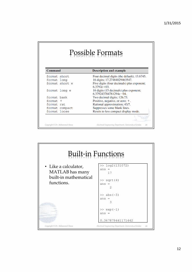
Built-in Functions

• Like a calculator, MATLAB has many built-in mathematical functions.

24

>> log2(131072)

ans =

17

>> sqrt(4)

ans =

2

>> abs(-3)

ans =

3

>> exp(-1)

ans =

0.367879441171442

1/31/2015

13


Common Built-in Functions

25


Exercise: Discussed Later…

x = 0:pi/100:2*pi;

y = sin(x);

plot(x,y)

• By the way, what is

the purpose of the semicolon at the end of the command?

26

1/31/2015

14


Exercise: Discussed Later…

x = 0:pi/100:2*pi;

y = sin(x);

plot(x,y)

0 1 2 3 4 5 6 7-1

-0.8

-0.6

-0.4

-0.2

0

0.2

0.4

0.6

0.8

1

27


Exercise 2: Discussed Later…

[X,Y] = meshgrid(-10:0.25:10,-10:0.25:10);

f = sinc(sqrt((X/pi).^2+(Y/pi).^2));

surf(X,Y,f);

axis([-10 10 -10 10 -0.3 1])

28

1/31/2015

15


Exercise 2: Discussed Later…

[X,Y] = meshgrid(-10:0.25:10,-10:0.25:10);

f = sinc(sqrt((X/pi).^2+(Y/pi).^2));

surf(X,Y,f);

axis([-10 10 -10 10 -0.3 1])

-10

-5

0

5

10

-10

-5

0

5

10

-0.2

0

0.2

0.4

0.6

0.8

1

xy

sin

c (

R)

29


To Know More: help>> help

HELP topics:

matlab\general - General purpose commands.

matlab\ops - Operators and special characters.

matlab\lang - Programming language constructs.

matlab\elmat - Elementary matrices and matrix manipulation.

matlab\randfun - Random matrices and random streams.

matlab\elfun - Elementary math functions.

matlab\specfun - Specialized math functions.

matlab\matfun - Matrix functions - numerical linear algebra.

matlab\datafun - Data analysis and Fourier transforms.

matlab\polyfun - Interpolation and polynomials.

matlab\funfun - Function functions and ODE solvers.

matlab\sparfun - Sparse matrices.

matlab\scribe - Annotation and Plot Editing.

matlab\graph2d - Two dimensional graphs.

matlab\graph3d - Three dimensional graphs.

matlab\specgraph - Specialized graphs.

matlab\graphics - Handle Graphics.

matlab\uitools - Graphical User Interface Tools.

matlab\strfun - Character strings.

matlab\imagesci - Image and scientific data

matlab\plottools - Graphical User Interface Tools.

fuzzy\fuzzy - Fuzzy Logic Toolbox

images\images - Image Processing Toolbox

signal\signal - Signal Processing Toolbox

wavelet\wavelet - Wavelet Toolbox

...

30

1/31/2015

16


Go inside: help>> help elfun

Elementary math functions.

Trigonometric.

sin - Sine.

sind - Sine of argument in degrees.

sinh - Hyperbolic sine.

asin - Inverse sine.

asind - Inverse sine, result in degrees.

asinh - Inverse hyperbolic sine.

cos - Cosine.

...

Exponential.

exp - Exponential.

expm1 - Compute exp(x)-1 accurately.

log - Natural logarithm.

log1p - Compute log(1+x) accurately.

log10 - Common (base 10) logarithm.

log2 - Base 2 logarithm and dissect floating point num.

pow2 - Base 2 power and scale floating point number.

realpow - Power that will error out on complex result.

reallog - Natural logarithm of real number.

...

Rounding and remainder.

fix - Round towards zero.

floor - Round towards minus infinity.

ceil - Round towards plus infinity.

round - Round towards nearest integer.

mod - Modulus (signed remainder after division).

rem - Remainder after division.

sign - Signum.

31


For a specific function: help exp

>> help exp

EXP Exponential.

EXP(X) is the exponential of the elements of X, e to the X.

For complex Z=X+i*Y, EXP(Z) = EXP(X)*(COS(Y)+i*SIN(Y)).

See also expm1, log, log10, expm, expint.

Overloaded methods:

codistributed/exp

fints/exp

Reference page in Help browser

doc exp

32

1/31/2015

17


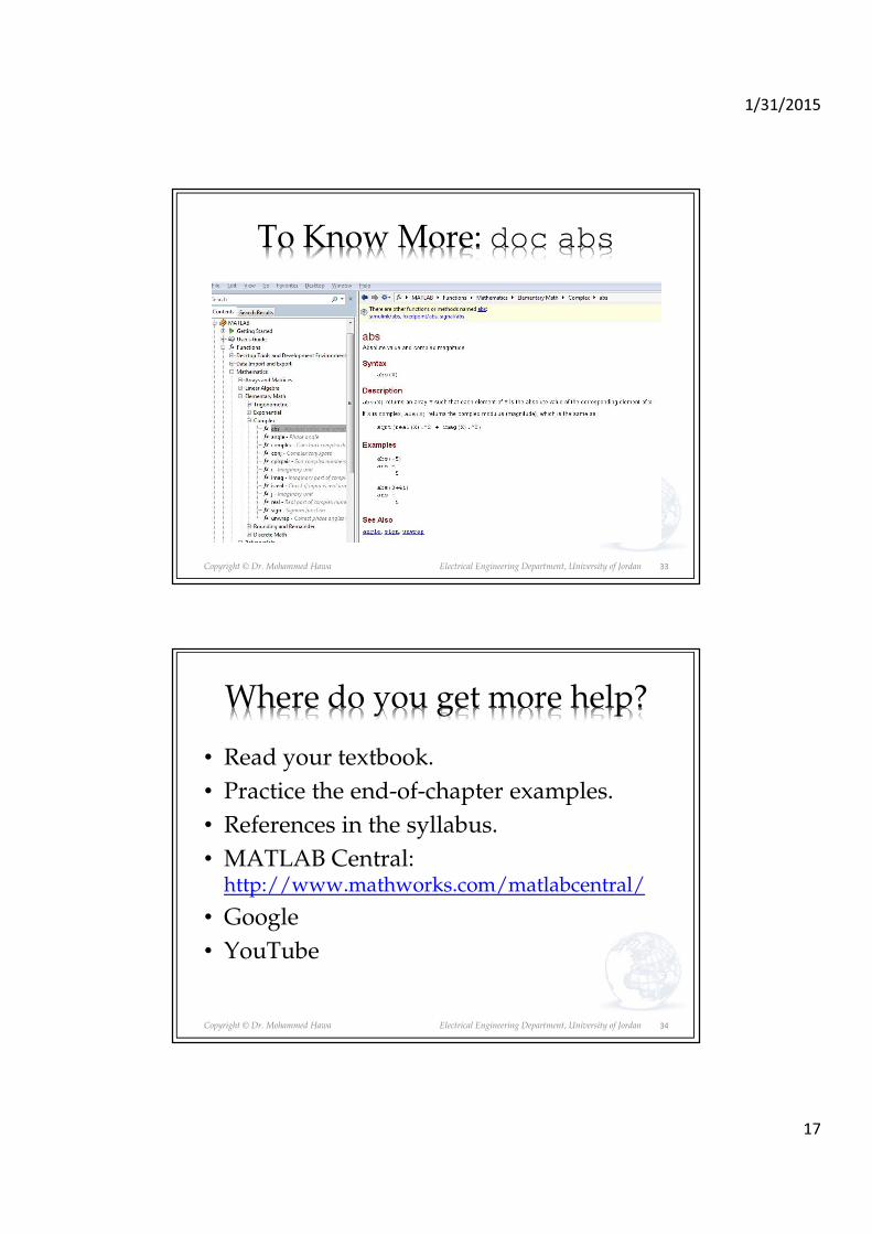
To Know More: doc abs

33


Where do you get more help?

• Read your textbook.

• Practice the end-of-chapter examples.

• References in the syllabus.

• MATLAB Central:http://www.mathworks.com/matlabcentral/

• Google

• YouTube

34

1/31/2015

1

Lecture 2: Variables, Vectors and Matrices in MATLAB



EE201: Computer Applications. See Textbook Chapter 1 and Chapter 2.


Variables in MATLAB• Just like other programming

languages, you can define variables in which to store values.

• All variables can by default hold matrices with scalar or complex numbers in them.

• You can define as many variables as your PC memory can hold.

• Values in variables can be inspected, used and changed

• Variable names are case-sensitive, and show up in the Workspace.

>> A = 5

A =

5

>> d = 7

d =

7

>> LightSpeed = 3e8

LightSpeed =

300000000

2

1/31/2015

2


Variables

• You can change the value in the variable by over-writing it with a new value

• Remember that variables are case-sensitive (easy to make a mistake)

• Always left-to right>> variable = expression

>> a = 7

a =

7

>> b = 12

b =

12

>> b = 14

b =

14

>> B = 88

B =

88

>> c = a + b

c =

21

>> c = a / b

c =

0.5000

3


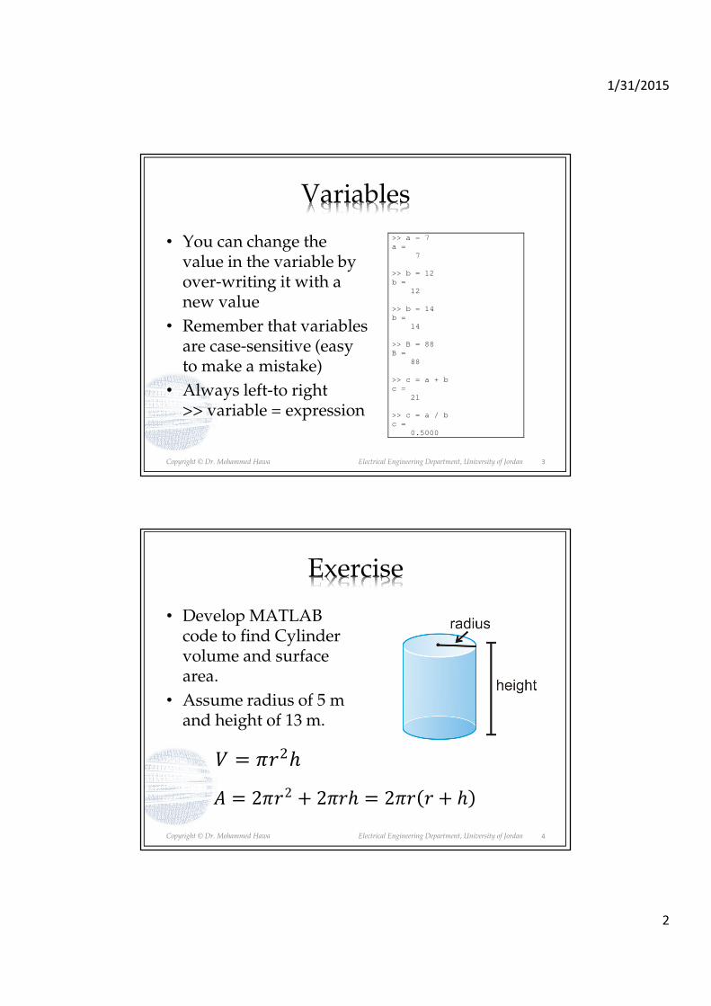
Exercise

• Develop MATLAB code to find Cylinder volume and surface area.

• Assume radius of 5 m and height of 13 m.

� = ��2ℎ

� = 2��2 + 2��ℎ = 2�� + ℎ�

4

1/31/2015

3


Solution

5

>> r = 5

r =

5

>> h = 13

h =

13

>> Volume = pi * r^2 * h

Volume =

1.0210e+003

>> Area = 2 * pi * r * (r + h)

Area =

565.4867


Useful MATLAB commands

6

1/31/2015

4


Vectors and Matrices (Arrays)

• So far we used MATLAB variables to store a single value.

• We can also create MATLAB arrays that hold multiple values– List of values (1D array) called Vector

– Table of values (2D array) called Matrix

• Vectors and matrices are used extensively when solving engineering and science problems.

7


Row Vector

• Row vectors are special cases of matrices.

• This is a 7-element row vector (1 × 7 matrix).

• Defined by enclosing numbers within square brackets [ ] and separating them by , or a space.

>> C = [10, 11, 13, 12, 19, 16, 17]

C =

10 11 13 12 19 16 17

>> C = [10 11 13 12 19 16 17]

C =

10 11 13 12 19 16 17

8

1/31/2015

5


Column Vector

• Column vectors are special cases of matrices.

• This is a 7-element column vector (7 × 1 matrix).

• Defined by enclosing numbers within [ ] and separating them by semicolon ;

>> R = [10; 11; 13; 12; 19; 16; 17]

R =

10

11

13

12

19

16

17

9


Matrix• This is a 3 × 4-element matrix.• It has 3 rows and 4 columns (dimension 3 × 4).• Spaces or commas separate elements in different columns,

whereas semicolons separate elements in different rows.• A dimension n × n matrix is called square matrix.

>> M = [1, 3, 2, 9; 6, 7, 8, 1; 7, 4, 6, 0]

M =

1 3 2 9

6 7 8 1

7 4 6 0

>> M = [1 3 2 9; 6 7 8 1; 7 4 6 0]

M =

1 3 2 9

6 7 8 1

7 4 6 0

10

1/31/2015

6


Transpose of a Matrix

• The transpose operation interchanges the rows and columns of a matrix.

• For an m × n matrix A the new matrix AT (read “ A transpose” ) is an n × m matrix.

• In MATLAB, the A’ command is used for transpose.

11


Exercise

>> A = [1 2 3; 5 6 7]

A =

1 2 3

5 6 7

>> A'

ans =

1 5

2 6

3 7

>> B = [5 6 7 8]

B =

5 6 7 8

>> B'

ans =

5

6

7

8

• What happens to a row vector when transposed?

• What happens to a column vector when transposed?

12

1/31/2015

7


Useful Functionslength(A) Returns either the number of elements of A if A

is a vector or the largest value of m or n if A is an m × n matrix

size(A) Returns a row vector [m n] containing the sizes of the m × n matrix A.

max(A) For vectors, returns the largest element in A. For matrices, returns a row vector containing the maximum element from each column.

If any of the elements are complex, max(A) returns the elements that have the largest magnitudes.

[v,k] = max(A) Similar to max(A) but stores the maximum values in the row vector v and their indices in the row vector k.

min(A)

and [v,k] = min(A)

Like max but returns minimum values.

13


More Useful Functions

sort(A) Sorts each column of the array A in ascending order and returns an array the same size as A.

sort(A,DIM,MODE) Sort with two optional parameters: DIM selects a dimension along which to sort. MODE is sort direction ('ascend' or 'descend').

sum(A) Sums the elements in each column of the array A and returns a row vector containing the sums.

sum(A,DIM) Sums along the dimension DIM.

14

1/31/2015

8


Exercises>> M = [1 6 4; 3 7 2]

>> size(M)

>> length(M)

>> max(M)

>> [a,b] = max(M)

>> sort(M)

>> sort(M, 1, 'descend')

>> sum(M)

>> sum(M, 2)

>> X = [4 9 2 5]

X =

4 9 2 5

>> length(X)

ans =

4

>> size(X)

ans =

1 4

>> min(X)

ans =

2

15


Solution>> M = [1 6 4; 3 7 2]

M =

1 6 4

3 7 2

>> size(M)

ans =

2 3

>> length(M)

ans =

3

>> max(M)

ans =

3 7 4

>> [a,b] = max(M)

a =

3 7 4

b =

2 2 1

>> sort(M)

ans =

1 6 2

3 7 4

>> sort(M, 1, 'descend')

ans =

3 7 4

1 6 2

>> sum(M)

ans =

4 13 6

>> sum(M, 2)

ans =

11

12

16

1/31/2015

9


The Variable Editor [from Workspace or openvar('A')]

17


Creating Big Matrices

• What if you want to create a Matrix that contains 1000 element (or more)?

• Writing each element by hand is difficult, time-consuming and error-prone.

• MATLAB allows simple ways to quickly create matrices, such as:

• Using the colon : operator (very popular).

• Using linspace() and logspace() functions (less popular, but useful).

18

1/31/2015

10


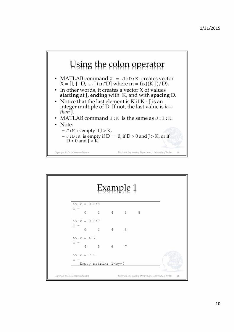
Using the colon operator

• MATLAB command X = J:D:K creates vector X = [J, J+D, ..., J+m*D] where m = fix((K-J)/D).

• In other words, it creates a vector X of values starting at J, ending with K, and with spacing D.

• Notice that the last element is K if K - J is an integer multiple of D. If not, the last value is less than J.

• MATLAB command J:K is the same as J:1:K.• Note:

– J:K is empty if J > K.– J:D:K is empty if D == 0, if D > 0 and J > K, or if

D < 0 and J < K.

19


Example 1

>> x = 0:2:8

x =

0 2 4 6 8

>> x = 0:2:7

x =

0 2 4 6

>> x = 4:7

x =

4 5 6 7

>> x = 7:2

x =

Empty matrix: 1-by-0

20

1/31/2015

11


Example 2

>> x = 7:-1:2

x =

7 6 5 4 3 2

>> x = 5:0.1:5.9

x =

Columns 1 through 5

5.0000 5.1000 5.2000 5.3000 5.4000

Columns 6 through 10

5.5000 5.6000 5.7000 5.8000 5.9000

>> y = 5:0.1:5.9; % what happened here?!

>>

>> % now create a ‘column’ vector from 1 to 10 using :

21


Alternatives to colon

• linspace command creates a linearly spaced row vector, but instead you specify the number of values rather than the increment.

• The syntax is linspace(x1,x2,n), where x1 and x2 are the lower and upper limits and n is the number of points.

• If n is omitted, the number of points defaults to 100.• logspace command creates an array of

logarithmically spaced elements.• Its syntax is logspace(a,b,n), where n is the

number of points between 10a and 10b. • If n is omitted, the number of points defaults to 50.

22

1/31/2015

12


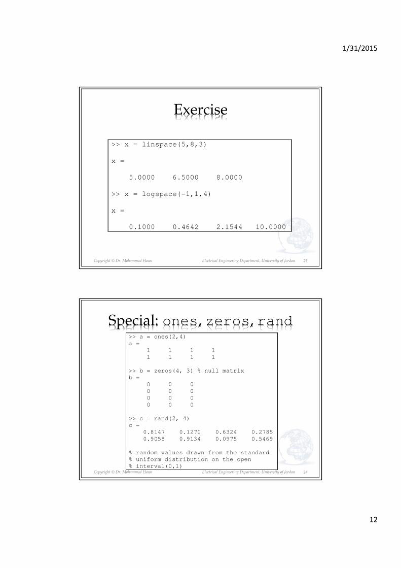
Exercise

>> x = linspace(5,8,3)

x =

5.0000 6.5000 8.0000

>> x = logspace(-1,1,4)

x =

0.1000 0.4642 2.1544 10.0000

23


Special: ones, zeros, rand>> a = ones(2,4)

a =

1 1 1 1

1 1 1 1

>> b = zeros(4, 3) % null matrix

b =

0 0 0

0 0 0

0 0 0

0 0 0

>> c = rand(2, 4)

c =

0.8147 0.1270 0.6324 0.2785

0.9058 0.9134 0.0975 0.5469

% random values drawn from the standard

% uniform distribution on the open

% interval(0,1)

24

1/31/2015

13


Null and Identity Matrix

>> eye(4) % identity matrix

ans =

1 0 0 0

0 1 0 0

0 0 1 0

0 0 0 1

>> A = [1 2 3; 4 5 6; 7 8 9]

A =

1 2 3

4 5 6

7 8 9

>> I = eye(3)

I =

1 0 0

0 1 0

0 0 1

>> A*I

ans =

1 2 3

4 5 6

7 8 9

25


Matrix Determinant & Inverse

>> A = [1 2 3; 2 3 1; 3 2 1]

A =

1 2 3

2 3 1

3 2 1

>> det(A) % determinant

ans =

-12

>> inv(A) % inverse

ans =

-0.0833 -0.3333 0.5833

-0.0833 0.6667 -0.4167

0.4167 -0.3333 0.0833

>> A^-1

ans =

-0.0833 -0.3333 0.5833

-0.0833 0.6667 -0.4167

0.4167 -0.3333 0.0833

26

1/31/2015

14


Accessing Matrix Elements

>> C = [10, 11, 13, 12, 19, 16, 17]

C =

10 11 13 12 19 16 17

>> C(4)

ans =

12

>> C(1,4)

ans =

12

>> C(20)

??? Index exceeds matrix dimensions.

27


Notes

• Use () not [] to access matrix elements.

• The row and column indices are NOT zero-based, like in C/C++.

• The first is row number, followed by the column number.

• For matrices and vectors, you can use one of three indexing methods: matrix row and column indexing; linear indexing; and logical indexing.

• You can also use ranges (shown later).

28

1/31/2015

15


Accessing Matrix Elements>> M = [1, 3, 2, 9; 6, 7, 8, 1; 7, 4, 6, 0]

M =

1 3 2 9

6 7 8 1

7 4 6 0

>> M(2, 3)

ans =

8

>> M(3, 1)

ans =

7

>> M(0, 1)

??? Subscript indices must either be real

positive integers or logicals.

>> M(9)

ans =

6

29


Matrix Linear Indexing

30

1/31/2015

16


Indexing: Sub-matrix

• v(2:5) represents the second through fifth elements– i.e., v(2), v(3), v(4), v(5).

• v(2:end) represents the second till last element of v. • v(:) represents all the row or column elements of vector v.

• A(:,3) denotes all elements in the third column of matrix A.• A(:,2:5) denotes all elements in the second through fifth

columns of A.• A(2:3,1:3) denotes all elements in the second and third

rows that are also in the first through third columns.• A(end,:) all elements of the last row in A.• A(:,end) all elements of the last column in A.• v = A(:) creates a vector v consisting of all the columns of A

stacked from first to last.

31


Exercise>> v = 10:10:70

v =

10 20 30 40 50 60 70

>> v(2:5)

ans =

20 30 40 50

>> v(2:end)

ans =

20 30 40 50 60 70

>> v(:)

ans =

10

20

30

40

50

60

70

32

1/31/2015

17


Exercise>> A = [4 10 1 6 2; 8 1.2 9 4 25; 7.2 5 7 1

11; 0 0.5 4 5 56; 23 83 13 0 10]

A =

4.0000 10.0000 1.0000 6.0000 2.0000

8.0000 1.2000 9.0000 4.0000 25.0000

7.2000 5.0000 7.0000 1.0000 11.0000

0 0.5000 4.0000 5.0000 56.0000

23.0000 83.0000 13.0000 0 0.0000

>> A(:,3)

ans =

1

9

7

4

13

>> A(:,2:5)

ans =

10.0000 1.0000 6.0000 2.0000

1.2000 9.0000 4.0000 25.0000

5.0000 7.0000 1.0000 11.0000

0.5000 4.0000 5.0000 56.0000

83.0000 13.0000 0 10.0000

>> A(2:3,1:3)

ans =

8.0000 1.2000 9.0000

7.2000 5.0000 7.0000

>> A(end,:)

ans =

23 83 13 0 10

>> A(:,end)

ans =

2

25

11

56

10

>> v = A(:)

v =

4.0000

8.0000

7.2000

0

23.0000

10.0000

1.2000

5.0000

0.5000

83.0000

1.0000

9.0000

7.0000

4.0000

13.0000

6.0000

4.0000

1.0000

5.0000

0

2.0000

25.0000

11.0000

56.0000

10.0000

33


Linear indexing: Advanced

>> A = 5:5:50

A =

5 10 15 20 25 30 35 40 45 50

>> A([1 3 6 10])

ans =

5 15 30 50

>> A([1 3 6 10]')

ans =

5 15 30 50

>> A([1 3 6; 7 9 10])

ans =

5 15 30

35 45 50

% indexing into a vector with a nonvector,

the shape of the indices is honored

34

1/31/2015

18


Linear indexing is useful: find>> A = [1 2 3; 4 5 6; 7 8 9]

A =

1 2 3

4 5 6

7 8 9

>> B = find(A > 5) % returns linear index

B =

3

6

8

9

>> A(B) % same as A( find(A > 5) )

ans =

7

8

6

9

35


Advanced: Logical indexing>> A = [1 2 3; 4 5 6; 7 8 9]

A =

1 2 3

4 5 6

7 8 9

>> B = logical([0 1 0; 1 0 1; 0 0 1])

B =

0 1 0

1 0 1

0 0 1

>> A(B)

ans =

4

2

6

9

36

1/31/2015

19


Logical indexing is also useful! >> A = [1 2 3; 4 5 6; 7 8 9]

A =

1 2 3

4 5 6

7 8 9

>> B = (A > 5) % true or false

B =

0 0 0

0 0 1

1 1 1

>> A(B) % same as A( A > 5 )

ans =

7

8

6

9

37


Subscripting Examples

38

1/31/2015

20


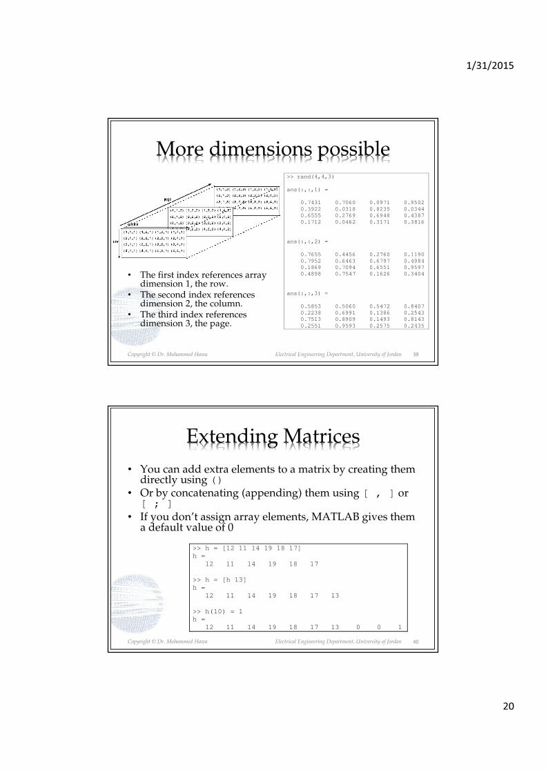
More dimensions possible>> rand(4,4,3)

ans(:,:,1) =

0.7431 0.7060 0.0971 0.9502

0.3922 0.0318 0.8235 0.0344

0.6555 0.2769 0.6948 0.4387

0.1712 0.0462 0.3171 0.3816

ans(:,:,2) =

0.7655 0.4456 0.2760 0.1190

0.7952 0.6463 0.6797 0.4984

0.1869 0.7094 0.6551 0.9597

0.4898 0.7547 0.1626 0.3404

ans(:,:,3) =

0.5853 0.5060 0.5472 0.8407

0.2238 0.6991 0.1386 0.2543

0.7513 0.8909 0.1493 0.8143

0.2551 0.9593 0.2575 0.2435

• The first index references array dimension 1, the row.

• The second index references dimension 2, the column.

• The third index references dimension 3, the page.

39


Extending Matrices

• You can add extra elements to a matrix by creating them directly using ()

• Or by concatenating (appending) them using [ , ] or [ ; ]

• If you don’t assign array elements, MATLAB gives them a default value of 0

>> h = [12 11 14 19 18 17]

h =

12 11 14 19 18 17

>> h = [h 13]

h =

12 11 14 19 18 17 13

>> h(10) = 1

h =

12 11 14 19 18 17 13 0 0 1

40

1/31/2015

21


Example>> a = [2 4 20]

a =

2 4 20

>> b = [9, -3, 6]

b =

9 -3 6

>> [a b]

ans =

2 4 20 9 -3 6

>> [a, b]

ans =

2 4 20 9 -3 6

>> [a; b]

ans =

2 4 20

9 -3 6

41


Functions on Arrays

• Standard MATLAB functions (sin, cos, exp, log, etc) can apply to vectors and matrices as well as scalars.

• They operate on array arguments to produce an array result the same size as the array argument x.

• These functions are said to be vectorized functions.• In this example y is [sin(1), sin(2), sin(3)]• So, when writing functions (later lectures) remember

input might be a vector or matrix.

>> x = [1, 2, 3]

x =

1 2 3

>> y = sin(x)

y =

0.8415 0.9093 0.1411

42

1/31/2015

22


Exercise>> x = linspace(0, 2*pi, 9) % OR x = linspace(0, 2*pi, 31)

x =

0 0.7854 1.5708 2.3562 3.1416 3.9270 4.7124 5.4978 6.2832

>> y = sin(x)

y =

0 0.7071 1.0000 0.7071 0.0000 -0.7071 -1.0000 -0.7071 -0.0000

>> plot(x,y)

43


Matrix vs. Array Arithmetic

• Multiplying and dividing vectors and matrices is different than multiplying and dividing scalars (or arrays of scalars).

• This is why MATLAB has two types of arithmetic operators:– Array operators: where the arrays operated on

have the same size. The operation is done element-by-element (for all elements).

– Matrix operators: dedicated for matrices and vectors. Operations are done using the matrix as a whole.

44

1/31/2015

23


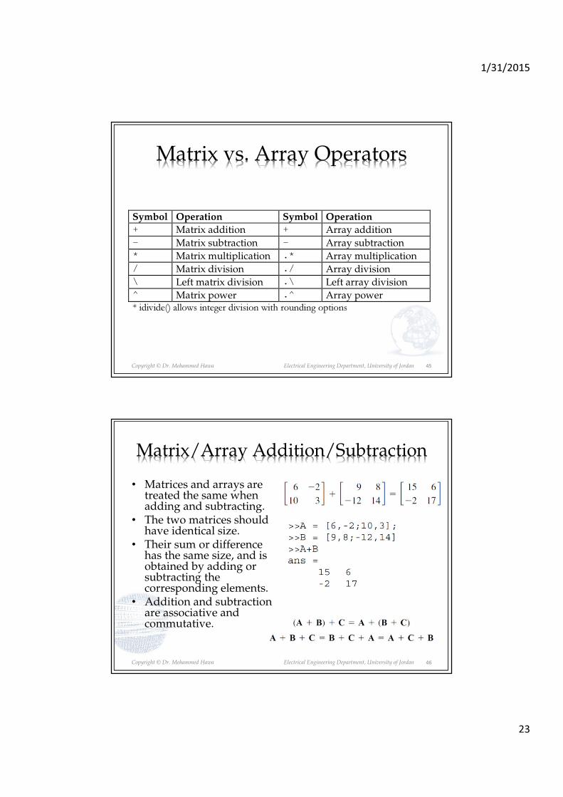
Matrix vs. Array Operators

Symbol Operation Symbol Operation + Matrix addition + Array addition - Matrix subtraction - Array subtraction * Matrix multiplication .* Array multiplication / Matrix division ./ Array division \ Left matrix division .\ Left array division ^ Matrix power .^ Array power * idivide() allows integer division with rounding options

45


Matrix/Array Addition/Subtraction

• Matrices and arrays are treated the same when adding and subtracting.

• The two matrices should have identical size.

• Their sum or difference has the same size, and is obtained by adding or subtracting the corresponding elements.

• Addition and subtraction are associative and commutative.

46

1/31/2015

24


More …

• A scalar value at either side of the operator is expanded to an array of the same size as the other side of the operator.

47


Array Multiplication

• Element-by-element multiplication.

• Only for arrays that are the same size.

• Use the .* operator not the * operator.

• Not the same as matrix multiplication.

• Useful in programming, but students make the mistake of using *

48

1/31/2015

25


Using Array Multiplication (Plot)

• Plot the following function:

• Notice the use of .* operator

0 0.05 0.1 0.15 0.2 0.25 0.3 0.35 0.4 0.45 0.5-0.2

0

0.2

0.4

0.6

0.8

1

1.2

>> t = 0:0.003:0.5;

>> y = exp(-8*t).*sin(9.7*t+pi/2);

>> plot(t,y)

49


Matrix Multiplication

• If A is an n × mmatrix and B is a m × p matrix, their matrix product AB is an n × p matrix, in which the m entries across the rows of A are multiplied with the m entries down the columns of B.

• In general, AB ≠ BA for matrices. Be extra careful.

50

1/31/2015

26


Matrix Multiplication

>> A = [6,-2;10,3;4,7];

>> B = [9,8;-5,12];

>> A*B

ans =

64 24

75 116

1 116

51


Array Division

• Element-by-element division.

• Only for arrays that are the same size.

• Use the ./ operator not the / operator.

• Not the same as matrix division.

• Useful in programming, but students make the mistake of using /

52

1/31/2015

27


Matrix Division

• An n × n square matrix B is called invertible (also nonsingular) if there exists an n × n matrix B-1

such that their multiplication is the identity matrix.

�

�= � �

−1

� �−1

= �

53


Matrix Division

>> A = [1 2 3; 3 2 1; 2 1 3];

>> B = [4 5 6; 6 5 4; 4 6 5];

>> A/B

ans =

0.7000 -0.3000 0

-0.3000 0.7000 0.0000

1.2000 0.2000 -1.0000

>> format rat

>> A/B

ans =

7/10 -3/10 0

-3/10 7/10 *

6/5 1/5 -1

54

1/31/2015

28


Matrix Left Division

• Use the left division operator (\) (back slash) to solve sets of linear algebraic equations.

• If A is n × n matrix and B is a column vector with nelements, then x = A\B is the solution to the equation Ax = B.

• A warning message is displayed if A is badly scaled or nearly singular.

55


Homework: Mesh AnalysisKVL @ mesh 2:

1(i2 − i1) + 2i2 + 3(i2 − i3) = 0KVL @ supermesh 1/3:

−7 +1(i1 − i2) + 3(i3 − i2) + 1i3 = 0@ current source:

7 = i1 − i3

Three equations:−i1 + 6i2 − 3i3 = 0i1 − 4i2 + 4i3 = 7i1 − i3 = 7Solution: i1 = 9A, i2 = 2.5A, i3 = 2A

56

1/31/2015

29


Just between us…

• Matrix division and matrix left division are related in MATLAB by the equation:

B/A = (A'\B')' % reversing

• To see the details, type: doc mldivideor type: doc mrdivide

57


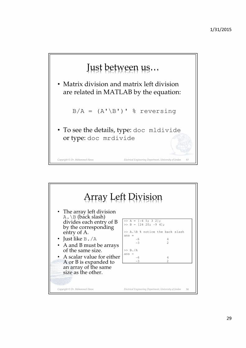
Array Left Division

• The array left division A.\B (back slash) divides each entry of B by the corresponding entry of A.

• Just like B./A• A and B must be arrays

of the same size. • A scalar value for either

A or B is expanded to an array of the same size as the other.

>> A = [-4 5; 3 2];

>> B = [24 20; -9 4];

>> A.\B % notice the back slash

ans =

-6 4

-3 2

>> B./A

ans =

-6 4

-3 2

58

1/31/2015

30


Array Power

59


Matrix Power

• A^k computes matrix power (exponent).

• In other words, it multiplies matrix A by itself k times.

• The exponent k requires a positive, real-valued integer value.

• Remember: this is repeated matrixmultiplication

>> A = [1 2; 3 4];

>> A^3

ans =

37 54

81 118

>> A*A*A

ans =

37 54

81 118

60

1/31/2015

31


Matrix Manipulation Functions

• diag: Diagonal matrices and diagonal of a matrix.

• det: Matrix determinant

• inv: Matrix inverse

• cond: Matrix condition number (for inverse)

• fliplr: Flip matrices left-right

• flipud: Flip matrices up and down

• repmat: Replicate and tile a matrix

61


Matrix Manipulation Functions

• rot90: rotate matrix 90º

• tril: Lower triangular part of a matrix

• triu: Upper triangular part of a matrix

• cross: Vector cross product

• dot: Vector dot product

• eig: Evaluate eigenvalues and eigenvectors

• rank: Rank of matrix

62

1/31/2015

32


Exercise

63

>> fliplr(A)

ans =

3 2 1

6 5 4

9 8 7

>> flipud(A)

ans =

7 8 9

4 5 6

1 2 3

>> rot90(A)

ans =

3 6 9

2 5 8

1 4 7

>> A = [1 2 3; 4 5 6; 7 8 9]

A =

1 2 3

4 5 6

7 8 9

>> diag(A)

ans =

1

5

9

>> det(A)

ans =

6.6613e-016


Exercise

64

>> [V, D] = eig(A)

V =

-0.2320 -0.7858 0.4082

-0.5253 -0.0868 -0.8165

-0.8187 0.6123 0.4082

D =

16.1168 0 0

0 -1.1168 0

0 0 -0.0000

>> A = [1 2 3; 4 5 6; 7 8 9]

A =

1 2 3

4 5 6

7 8 9

>> tril(A)

ans =

1 0 0

4 5 0

7 8 9

>> triu(A)

ans =

1 2 3

0 5 6

0 0 9

1/31/2015

33


Exercise

• Define matrix A of dimension 2 by 4 whose (i,j) entries are A(i,j) = i+j

• Extract two 2 by 2 matrices A1 and A2 out of matrix A.

– A1 contains the first two columns of A

– A2 contains the last two columns of A

• Compute matrix B to be the sum of A1 and A2

• Compute the eigenvalues and eigenvectors of B

• Solve the linear system B x = b, where b has all entries = 2

• Compute the determinant of B, inverse of B, and the condition number of B

• NOTE: Use only MATLAB native functions for all above.

65


Solution>> b = [2; 2]

b =

2

2

>> B\b

ans =

-1.0000

1.0000

>> det(B)

ans =

-4

>> inv(B)

ans =

-1.5000 1.0000

1.0000 -0.5000

>> cond(B)

ans =

17.9443

>> A =[0 1 2 3; 1 2 3 4]

A =

0 1 2 3

1 2 3 4

>> A1 = A(:,1:2)

A1 =

0 1

1 2

>> A2 = A(:,3:4)

A2 =

2 3

3 4

>> B = A1 + A2

B =

2 4

4 6

66

1/31/2015

34


Homework

• Solve as many problems from Chapter 1 as you can

• Suggested problems:

• 1.3, 1.8, 1.15, 1.26, 1.30



• 2.3, 2.10, 2.13, 2.25, 2.26

67

2/7/2015

1

Lecture 3: Array Applications, Cells, Structures & Script Files



EE201: Computer Applications. See Textbook Chapter 2 and Chapter 3.


Euclidean Vectors

• An Euclidean vector (or geometric vector, or simply a vector) is a geometric entity that has both magnitude and direction.

• In physics, vectors are used to represent physical quantities that have both magnitude and direction, such as force, acceleration, electric field, etc.

• Vector algebra: adding and subtracting vectors, multiplying vectors, scaling vectors, etc.

2

2/7/2015

2


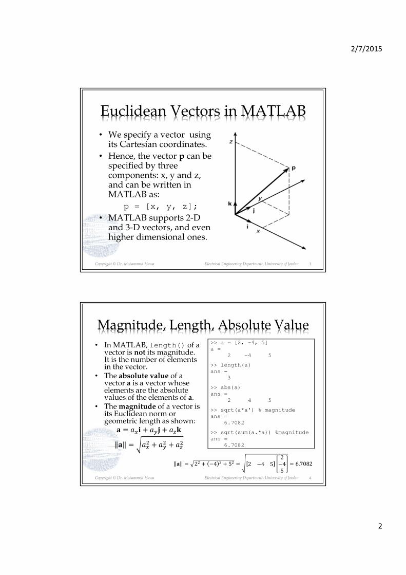
Euclidean Vectors in MATLAB

• We specify a vector using its Cartesian coordinates.

• Hence, the vector p can be specified by three components: x, y and z, and can be written in MATLAB as:

p = [x, y, z];

• MATLAB supports 2-D and 3-D vectors, and even higher dimensional ones.

3


Magnitude, Length, Absolute Value

• In MATLAB, length() of a vector is not its magnitude. It is the number of elements in the vector.

• The absolute value of a vector a is a vector whose elements are the absolute values of the elements of a.

• The magnitude of a vector is its Euclidean norm or geometric length as shown:

� � ��

� � ��

� � ��

‖�‖ = �22 + �−4�2 + 52 = ��2 −4 5� 2

−4

5

= 6.7082

4

>> a = [2, -4, 5]

a =

2 -4 5

>> length(a)

ans =

3

>> abs(a)

ans =

2 4 5

>> sqrt(a*a') % magnitude

ans =

6.7082

>> sqrt(sum(a.*a)) %magnitude

ans =

6.7082

2/7/2015

3


Vector Scaling

• For vector:� � ��

• Scaling this vector by a factor of 2 gives:

• � � 2�

� 2�� 2�� 2��

• This is just like MATLAB scalar multiplication of a vector:

• v = 2*[x, y, z];

5


Adding and Subtracting Vectors

• Vector addition by geometry: The parallelogram law.

• Or, mathematically:� � ��

� � ��

� � � � ��

� ��

� ��

• Same as vector addition and subtraction in MATLAB.

6

2/7/2015

4


Exercise>> a = [2 -4 6]

a =

2 -4 6

>> b = [3 -1 -1]

b =

3 -1 -1

>> c = a + b

c =

5 -5 5

>> d = a - b

d =

-1 -3 7

>> e = 2*a

e =

4 -8 12

7


Dot Product

• The dot product of vectors results in a scalar value.

• � ∙ �

� ��

� � � cos �

>> a = [2 -4 6];

>> b = [3 -1 -1];

>> c = a * b'

c =

4

>> c = sum(a .* b)

c =

4

>> c = dot(a, b)

c =

4

8

2/7/2015

5


Cross Product>> a = [2 -4 6];

>> b = [3 -1 -1];

>> cross(a, b)

ans =

10 20 10

>> syms x y z

>> det([x y z; 2 -4 6; 3 -1 -1])

ans =

10*x + 20*y + 10*z

>> cross([1 0 0], [0 1 0])

ans =

0 0 1

� � � � sin �

� � �

� � �

��

��

� � ��

��

��

� ��

��

9


Complex Numbers

10

>> a = 7 + 4j

a =

7.0000 + 4.0000i

>> [theta, rho] = cart2pol(real(a), imag(a))

theta =

0.5191

rho =

8.0623

>> rho = abs(a) % magnitude of complex number

rho =

8.0623

>> theta = atan2(imag(a), real(a))

theta =

0.5191

% atan2 is four quadrant inverse tangent

>> b = 3 + 4j

b =

3.0000 + 4.0000i

>> a+b

ans =

10.0000 + 8.0000i

>> a*b

ans =

5.0000 + 40.0000i

2/7/2015

6


Polynomials

• A polynomial can be written in the form:�� ⋯� ��

• Or more concisely:

��

�

��

• We can use MATLAB to find all the roots of the polynomial, i.e., the values of x that makes the polynomial equation equal 0.

11


Exercise

>> a = [1 -7 40 -34];

>> roots(a)

ans =

3.0000 + 5.0000i

3.0000 - 5.0000i

1.0000

>> poly([1 3+5i 3-5i])

ans =

1 -7 40 -34

• Polynomial Roots:x3 – 7x2 + 40x – 34 = 0

• Roots are x = 1, x = 3 ± 5i.

• We can also build polynomial coefficients from its roots.

• We can also multiply (convolution) and divide (deconvolution) two polynomials.

12

2/7/2015

7


Just for fun… Plot…

>> x = -2:0.01:5;

>> f = x.^3 - 7*(x.^2) + 40*x - 34;

>> plot(x, f)

-2 -1 0 1 2 3 4 5-150

-100

-50

0

50

100

150

13


Cell Array

• The cell array is an array in which each element is a cell. Each cell can contain an array.

• So, it is an array of different arrays.• You can store different classes of arrays in

each cell, allowing you to group data sets that are related but have different dimensions.

• You access cell arrays using the same indexing operations used with ordinary arrays, but using {} not ().

14

2/7/2015

8


Useful functions

C = cell(n) Creates n × n cell array C of empty matrices.

C = cell(n,m) Creates n × m cell array C of empty matrices.

celldisp(C) Displays the contents of cell array C.

cellplot(C) Displays a graphical representation of the cell array C.

C = num2cell(A) Converts a numeric array A into a cell array C.

iscell(C) Returns a 1 if C is a cell array; otherwise, returns a 0.

15


Exercise>> C = cell(3)

C =

[] [] []

[] [] []

[] [] []

>> D = cell(1, 3)

D =

[] [] []

>> A(1,1) = {'Walden Pond'};

>> A(1,2) = {[1+2i 5+9i]};

>> A(2,1) = {[60,72,65]};

>> A(2,2) = {[55,57,56;54,56,55;52,55,53]};

>> A

A =

'Walden Pond' [1x2 double]

[1x3 double] [3x3 double]

16

2/7/2015

9


Exercise (Continue)>> celldisp(A)

A{1,1} =

Walden Pond

A{2,1} =

60 72 65

A{1,2} =

1.0000 + 2.0000i 5.0000 + 9.0000i

A{2,2} =

55 57 56

54 56 55

52 55 53

>> B = {[2,4], [6,-9;3,5]; [7;2], 10}

B =

[1x2 double] [2x2 double]

[2x1 double] [ 10]

>> B{1,2}

ans =

6 -9

3 5

17


Structures (strcut.memebr)

18

2/7/2015

10


Create and Add to Structure>> student.name = 'John Smith';

>> student.SSN = '392-77-1786';

>> student.email = '[email protected]';

>> student.exam_scores = [67,75,84];

>> student

student =

name: 'John Smith'

SSN: '392-77-1786'

email: '[email protected]'

exam_scores: [67 75 84]

>> student(2).name = 'Mary Jones';

>> student(2).SSN = '431-56-9832';

>> student(2).email = '[email protected]';

>> student(2).exam_scores = [84,78,93];

>> student

student =

1x2 struct array with fields:

name

SSN

email

exam_scores

19


Investigate Structure>> student(2)

ans =

name: 'Mary Jones'

SSN: '431-56-9832'

email: '[email protected]'

exam_scores: [84 78 93]

>> fieldnames(student)

ans =

'name'

'SSN'

'email'

'exam_scores'

>> max(student(2).exam_scores)

ans =

93

>> isstruct(student)

ans =

1

20

2/7/2015

11


Script files

• You can save a particular sequence of MATLAB commands for reuse later in a script file (.m file)

• Each line is the same as typing a command in the command window.

• From the main menu, select File | New | Script, then save the file as mycylinder.m

21


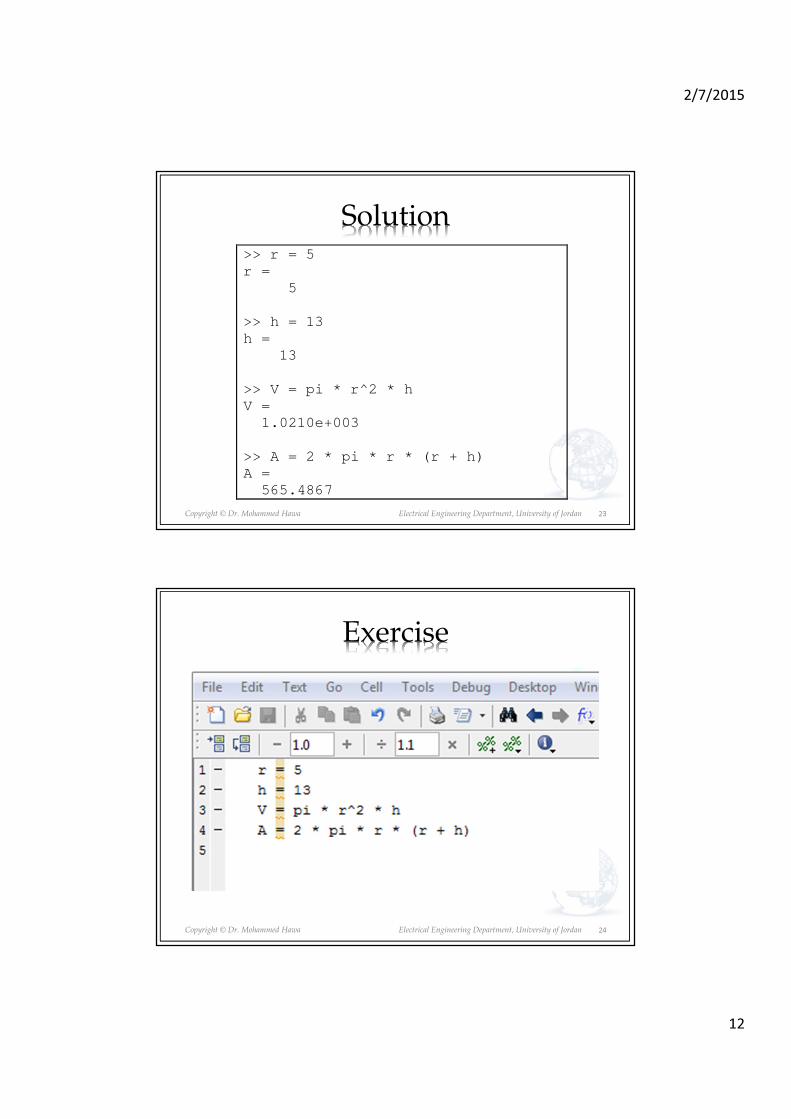
Remember Example?

• Develop MATLAB code to find Cylinder volume and surface area.

• Assume radius of 5 m and height of 13 m.

� = ��2ℎ

� = 2��2 + 2��ℎ = 2�� + ℎ�

22

2/7/2015

12


Solution

23

>> r = 5

r =

5

>> h = 13

h =

13

>> V = pi * r^2 * h

V =

1.0210e+003

>> A = 2 * pi * r * (r + h)

A =

565.4867

Copyright © Dr. Mohammed Hawa Electrical Engineering Department, University of Jordan 24

Exercise

2/7/2015

13


Be ware…• Script File names MUST begin with a letter, and

may include digits and the underscore character.• Script File names should NOT:

– include spaces– start with a number– use the same name as a variable or an existing

command

• If you do any of the above you will get unusual errors when you try to run your script.

• You can check to see if a command, function or file name already exists by using the existcommand.

25


Running .m files

• Run sequence of commands by typing

mycylinder

in the command window

• Make sure the current folder is set properly

26

>> mycylinder

r =

5

h =

13

V =

1.0210e+003

A =

565.4867

2/7/2015

14


When you type mycylinder

When multiple commands have the same name in the current scope (scope includes current file, optional private subfolder, current folder, and the MATLAB path), MATLAB uses this precedence order:

1. Variables in current workspace: Hence, if you create a variable with the same name as a function, MATLAB cannot run that function until you clear the variable from memory.

2. Nested functions within current function

3. Local functions within current file

4. Functions in current folder

5. Functions elsewhere on the path, in order of appearance

Precedence of functions within the same folder depends on file type:

1. MATLAB built-in functions have precedence

2. Then Simulink models

3. Then program files with .m extension

27


Comments in MATLAB

• Comment lines start with a % not //• Comments are not executed by MATLAB; it is

there for people reading the code.• Helps people understand what the code is doing

and why!• Comments are VERY IMPORTANT. • Comment anything that is not easy to understand.• Good commenting is a huge help when

maintaining/fixing/extending code.• Header comments show up when typing the help

command.

28

2/7/2015

15


Bad vs. Good Comments/Code

% set x to zero

x = 0

% calculate y

y = x * 9/5 + 32

% Convert freezing point of

% water from celsius to

% farenheit

c = 0

f = c * 9/5 + 32

29


Exercise

30

2/7/2015

16


Header comments

>> help temperature

temperature.m Convert the boiling point for

water from degrees Celsius (C) to Farenheit (F)

Author: Dr. Mohammed Hawa

>> temperature

C =

100

F =

212

31


Simple User Interaction: I/O

• Use input command to get input from the user and store it in a variable:

h = input('Enter the height:')

• MATLAB will display the message enclosed in quotes, wait for input and then store the entered value in the variable

32

2/7/2015

17


Simple User Interaction: I/O

• Use disp command to show something to a user

disp('The area of the cylinder is: ')

disp(A)

• MATLAB will display any message enclosed in quotes and then the value of the variable.

33


Exercise

34

r = input('Enter the radius:');

h = input('Enter the height:');

V = pi * r^2 * h;

A = 2 * pi * r * (r + h);

disp('The volume of the cylinder is: ');

disp(V);

disp('The area of the cylinder is: ');

disp(A);

>> mycylinder

Enter the radius:5

Enter the height:13

The volume of the cylinder is:

1.0210e+003

The area of the cylinder is:

565.4867

2/7/2015

18


Summary

35


Homework

• The speed v of a falling object dropped with zero initial velocity is given as a function of time t by � � ��, where g is the gravitational acceleration.

• Plot v as a function of t for 0 ≪ � ≪ ��,

where tf is the final time entered by the user.

• Use a script file with proper comments.

36

2/7/2015

19


Solution

% Plot speed of a falling object % Author: Dr. Mohammed Hawa

g = 9.81; % Acceleration in SI units

tf = input('Enter final time in seconds:');

t = [0:tf/500:tf]; % array of 501 time instants v = g*t; % speed

plot(t,v); xlabel('t (sseconds)'); ylabel('v m/s)');

37


Homework



• 2.33, 2.34, 2.35, 2.36, 2.39, 2.41, 2.45, 2.48

38

2/7/2015

1

Lecture 4: Complex Numbers Functions, and Data Input





What is a Function?

• A MATLAB Function (e.g. y = func(x1, x2)) is like a script file, but with inputs and outputs provided automatically in the commend window.

• In MATLAB, functions can take zero, one, two or more inputs, and can provide zero, one, two or more outputs.

• There are built-in functions (written by the MATLAB team) and functions that you can define (written by you and stored in .m file).

• Functions can be called from command line, from wihtin a script, or from another function.

2

2/7/2015

2



Functions are Helpful

• Enable “divide and conquer” strategy– Programming task broken into smaller tasks

• Code reuse– Same function useful for many problems

• Easier to debug– Check right outputs returned for all possible

inputs

• Hide implementation– Only interaction via inputs/outputs, how it is

done (implementation) hidden inside the function.

4

2/7/2015

3


Finding Useful Functions

• You can use the lookfor command to find MATLAB functions that are relevant to your application.

• Example: >> lookfor imaginary

• Gets a list of functions that deal with imaginary numbers.

• i - Imaginary unit.

• j - Imaginary unit.

• complex - Construct complex result from real and imaginary parts.

• imag - Complex imaginary part.

5


Calling Functions

• Function names are case sensitive (meshgrid, meshGrid and MESHGRID are interpreted as different functions).

• Inputs (called function arguments or function parameters) can be either numbers or variables.

• Inputs are passed into the function inside of parentheses () separated by commas.

• We usually assign the output to variable(s) so we can use it later. Otherwise it is assigned to the built-in variable ans.

6

2/7/2015

4


Rules

• To evaluate sin 2 in MATLAB, we type sin(2), not sin[2]

• For example sin[x(2)] gives an error even if x is defined as an array.

• Inputs to functions in MATLAB can be sometimes arrays.

>> x = -3 + 4i;

>> mag_x = abs(x)

mag_x =

5

>> mag_y = abs(6 - 8i)

mag_y =

10

>> angle_x = angle(x)

angle_x =

2.2143

>> angle(x)

ans =

2.2143

>> x = [5,7,15]

x =

5 7 15

>> y = sqrt(x)

y =

2.2361 2.6458 3.8730

7


Function Composition

• Composition: Using a function as an argument of another function

• Allowed in MATLAB.

• Just check the number and placement of parentheses when typing such expressions.

• sin(sqrt(x)+1)

• log(x.^2 + sin(5))

8

2/7/2015

5


Which expression is correct?

• You want to find sin� � . What do you write?

• (sin(x))^2

• sin^2(x)

• sin^2x

• sin(x^2)

• sin(x)^2

• Solution: Only first and last expressions are correct.

9


Trigonometric Functions

10

2/7/2015

6


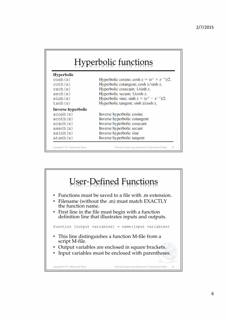
Hyperbolic functions

11


User-Defined Functions

• Functions must be saved to a file with .m extension. • Filename (without the .m) must match EXACTLY

the function name.• First line in the file must begin with a function

definition line that illustrates inputs and outputs.

function [output variables] = name(input variables)

• This line distinguishes a function M-file from a script M-file.

• Output variables are enclosed in square brackets.• Input variables must be enclosed with parentheses.

12

2/7/2015

7


Functions Names

• Function names may only use alphanumeric characters and the underscore.

• Functions names should NOT:– include spaces

– start with a number

– use the same name as an existing command

• Consider adding a header comment, just under the function definition (for help).

13


Exercise: Your Own pol2cart

• Make sure you set you Current Folder to Desktop (or where you saved the .m file).

14

2/7/2015

8


Test your newly defined function

>> [a, b] = polar_to_cartesian(3, pi)

a =

-3

b =

3.6739e-016

>> polar_to_cartesian(3, pi)

ans =

-3

>> [a, b] = polar_to_cartesian(3, pi/4)

a =

2.1213

b =

2.1213

>> [a, b] = polar_to_cartesian([3 3 3], [pi pi/4 pi/2])

a =

-3.0000 2.1213 0.0000

b =

0.0000 2.1213 3.0000

15


MATLAB has pol2cart>> help pol2cart

POL2CART Transform polar to Cartesian coordinates.

[X,Y] = POL2CART(TH,R) transforms corresponding elements of data

stored in polar coordinates (angle TH, radius R) to Cartesian

coordinates X,Y. The arrays TH and R must the same size (or

either can be scalar). TH must be in radians.

[X,Y,Z] = POL2CART(TH,R,Z) transforms corresponding elements of

data stored in cylindrical coordinates (angle TH, radius R, height

Z) to Cartesian coordinates X,Y,Z. The arrays TH, R, and Z must be

the same size (or any of them can be scalar). TH must be in radians.

Class support for inputs TH,R,Z:

float: double, single

See also cart2sph, cart2pol, sph2cart.

Reference page in Help browser

doc pol2cart

16

2/7/2015

9


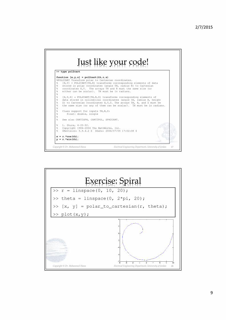
Just like your code!>> type pol2cart

function [x,y,z] = pol2cart(th,r,z)

%POL2CART Transform polar to Cartesian coordinates.

% [X,Y] = POL2CART(TH,R) transforms corresponding elements of data

% stored in polar coordinates (angle TH, radius R) to Cartesian

% coordinates X,Y. The arrays TH and R must the same size (or

% either can be scalar). TH must be in radians.

%

% [X,Y,Z] = POL2CART(TH,R,Z) transforms corresponding elements of

% data stored in cylindrical coordinates (angle TH, radius R, height

% Z) to Cartesian coordinates X,Y,Z. The arrays TH, R, and Z must be

% the same size (or any of them can be scalar). TH must be in radians.

%

% Class support for inputs TH,R,Z:

% float: double, single

%

% See also CART2SPH, CART2POL, SPH2CART.

% L. Shure, 4-20-92.

% Copyright 1984-2004 The MathWorks, Inc.

% $Revision: 5.9.4.2 $ $Date: 2004/07/05 17:02:08 $

x = r.*cos(th);

y = r.*sin(th);

17


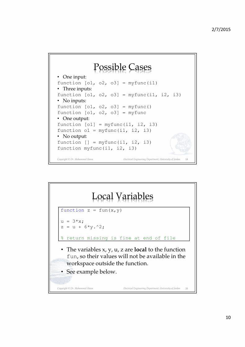
Exercise: Spiral>> r = linspace(0, 10, 20);

>> theta = linspace(0, 2*pi, 20);

>> [x, y] = polar_to_cartesian(r, theta);

>> plot(x,y);

18

2/7/2015

10


Possible Cases• One input:function [o1, o2, o3] = myfunc(i1)

• Three inputs:function [o1, o2, o3] = myfunc(i1, i2, i3)

• No inputs:function [o1, o2, o3] = myfunc()

function [o1, o2, o3] = myfunc

• One output:function [o1] = myfunc(i1, i2, i3)

function o1 = myfunc(i1, i2, i3)

• No output:function [] = myfunc(i1, i2, i3)

function myfunc(i1, i2, i3)

19


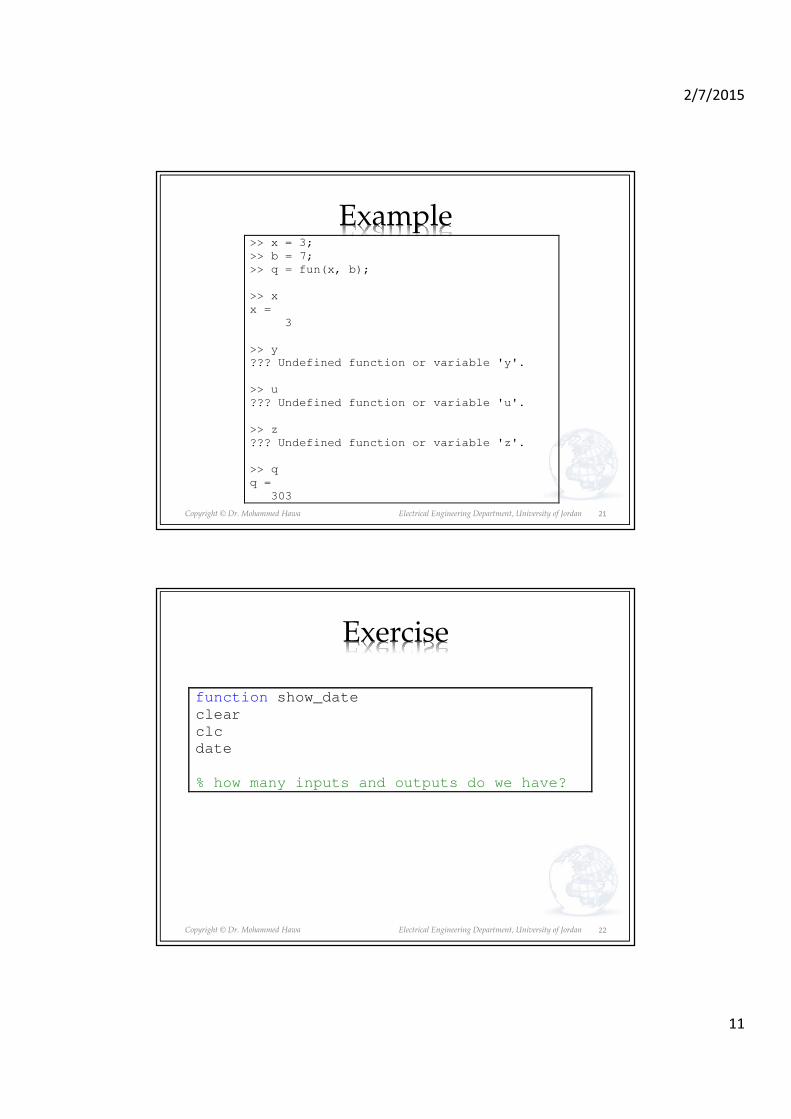
Local Variables

• The variables x, y, u, z are local to the function fun, so their values will not be available in the workspace outside the function.

• See example below.

function z = fun(x,y)

u = 3*x;

z = u + 6*y.^2;

% return missing is fine at end of file

20

2/7/2015

11


Example>> x = 3;

>> b = 7;

>> q = fun(x, b);

>> x

x =

3

>> y

??? Undefined function or variable 'y'.

>> u

??? Undefined function or variable 'u'.

>> z

??? Undefined function or variable 'z'.

>> q

q =

303

21


Exercise

function show_date

clear

clc

date

% how many inputs and outputs do we have?

22

2/7/2015

12


Homework

function [dist, vel] = drop(vO, t) % Compute the distance travelled and the % velocity of a dropped object, from % the initial velocity vO, and time t % Author: Dr. Mohammed Hawa

g = 9.80665; % gravitational acceleration (m/s^2) vel = g*t + vO; dist = 0.5*g*t.^2 + vO*t;

>> t = 0:0.1:5;

>> [distance_dropped, velocity] = drop(10, t);

>> plot(t, velocity)

23


Local vs. Global Variables

• The variables inside a function are local. Their scope is only inside the function that declares them.

• In other words, functions create their own workspaces.• Function inputs are also created in this workspace

when the function starts.• Functions do not know about any variables in any

other workspace.• Function outputs are copied from the function

workspace when the function ends.• Function workspaces are destroyed after the function

ends.– Any variables created inside the function “disappear”

when the function ends.

24

2/7/2015

13


Local vs. Global Variables

• You can, however, define global variables if you want using the global keyword.

• Syntax: global a x q

• Global variables are available to the basic workspace and to other functions that declare those variables global (allowing assignment to those variables from multiple functions).

25


Subfunctions

• An M-file may contain more than one user-defined function.• The first defined function in the file is called the primary

function, whose name is the same as the M-file name. • All other functions in the file are called subfunctions. They can

serve as subroutines to the primary function.• Subfunctions are normally “visible” only to the primary

function and other subfunctions in the same file; that is, they normally cannot be called by programs or functions outside the file.

• However, this limitation can be removed with the use of function handles.

• We normally use the same name for the primary function and its file, but if the function name differs from the file name, you must use the file name to invoke the function.

26

2/7/2015

14


Exercise

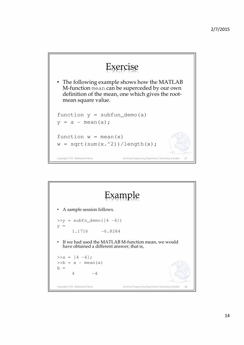
• The following example shows how the MATLAB M-function mean can be superceded by our own definition of the mean, one which gives the root-mean square value.

function y = subfun_demo(a)

y = a - mean(a);

function w = mean(x)

w = sqrt(sum(x.^2))/length(x);

27


Example

• A sample session follows.

>>y = subfn_demo([4 -4])

y =

1.1716 -6.8284

• If we had used the MATLAB M-function mean, we would have obtained a different answer; that is,

>>a = [4 -4];

>>b = a - mean(a)

b =

4 -4

28

2/7/2015

15


Function Handles

• You can create a function handle to any function by using the @ sign before the function name.

• You can then use the handle to reference the function.

function y = f1(x)

y = x + 2*exp(-x) - 3;

• You can pass the function as an argument to another function using the handle. Example: fzero function finds the zero of a function of a single variable x.

• >> x0 = 3; % initial guess

• >> fzero(@f1, x0)

29


Handle vs. Return Value

t = -1:0.1:5;

plot(t, f1(t));

• There is a zero near � � �0.5

and one near � � 3.

-1 0 1 2 3 4 5-1.5

-1

-0.5

0

0.5

1

1.5

2

2.5

30

2/7/2015

16


Exercise

fzero(@function,x0)

• where @function is the function handle, and x0 is a user-supplied initial guess for the zero.

>> fzero(@f1, -0.5)

ans =

-0.5831

>> fzero(@f1, 3)

ans =

2.8887

>> fzero(@sin, 0.1)

ans =

6.6014e-017

>> fzero(@cos, 2)

ans =

1.5708

>> pi/2

ans =

1.5708

31


Finding the Minimum

• The fminbnd function finds the minimum of a function of a single variable x in the interval x1 ≤ x ≤ x2.

• fminbnd(@function, x1, x2)

• fminbnd(@cos, 0, 4) returns 3.1416

• function y = f2(x)

• y = 1-x.*exp(-x);

• x = fminbnd(@f2, 0, 5) returns x = 1 • How would I find the min value of f2? (i.e. 0.6321)

32

2/7/2015

17


Exercise

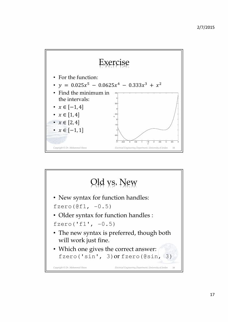
• For the function:

• � 0.025�� 0.0625�� 0.333��

• Find the minimum inthe intervals:

• � ∈ �1, 4

• � ∈ 1, 4

• � ∈ 2, 4

• � ∈ �1, 1

33


Old vs. New

• New syntax for function handles:

fzero(@f1, -0.5)

• Older syntax for function handles :

fzero('f1', -0.5)

• The new syntax is preferred, though both will work just fine.

• Which one gives the correct answer:fzero('sin', 3)or fzero(@sin, 3)

34

2/7/2015

18


The fminsearch function

• fminsearch finds minimum of a function of more than one variable.

• To find where the minimum of � � �� , define it in an M-file, using the vector x whose elements are x(1) = x and x(2) = y.

function f = f4(x)

f = x(1).*exp(-x(1).^2-x(2).^2);

• Suppose we guess that the minimum is near � � 0, � � 0.

>>fminsearch(@f4,[0,0])

ans =

-0.7071 0.000

• Thus the minimum occurs at � � 0.7071, � � 0.

35


Inline Function

• No need to save the function in an M-file.

• Useful for small size functions defined on the fly.

• You can use a string array to define the function.

• Anonymous functions are similar (see next).

>> f4 = inline('x.^2-4')

f4 =

Inline function:

f4(x) = x.^2-4

>> [x, value] = fzero(f4, 0)

x =

-2

value =

0

>> f5str = 'x.^2-4'; % string array

>> f5 = inline(f5str)

f5 =

Inline function:

f5(x) = x.^2-4

>> x = fzero(f5, 3)

x =

2

>> x = fzero('x.^2-4', 3)

x =

2

>> f6 = inline('x.*y')

f6 =

Inline function:

f6(x,y) = x.*y

36

2/7/2015

19


Anonymous functions

• Here is a simple function called sq to calculate the square of a number.

>> sq = @(x) x.^2;

>> sq = @(x) (x.^2)

sq =

@(x)(x.^2)

>> sq([5 7])

ans =

25 49

>> fminbnd(sq, -10, 10)

ans =

0

37


Exercise>> sqrtsum = @(x,y) sqrt(x.^2 + y.^2);

>> sqrtsum(3, 4)

ans =

5

>> A = 6; B = 4;

>> plane = @(x,y) A*x + B*y;

>> z = plane(2,8)

z =

44

>> f = @(x) x.^3; % try by hand!

>> g = @(x) 5*sin(x);

>> h = @(x) g(f(x));

>> h(2)

ans =

4.9468

38

2/7/2015

20


Variables in Anonymous Functions

• When the function is created MATLAB, it captures the values of these variables and retains those values for the lifetime of the function handle. If the values of A or B are changed after the handle is created, their values associated with the handle do not change.

• This feature has both advantages and disadvantages, so you must keep it in mind.

39


For Speed Use Handles

• The function handle provides speed improvements.

• Another advantage of using a function handle is that it provides access to subfunctions, which are normally not visible outside of their defining M-file.

40

2/7/2015

21


Importing Data: ASCII

• Make the ‘data’ folder your Current Folder.

• Delimited ASCII files are common to save data fromexperiments.

• dlmread/dlmwrite

>> a = dlmread('ascii.txt')

a =

1 2 3 4

5 6 7 8

9 10 11 12

41


Importing Data: Excel


• MATLAB can also read and write to Excel Files.

• xlsread/xlswrite

>> a = xlsread('data.xls')

a =

10 30 50 60

15 20 25 30

30 31 32 33

80 82 84 86

42

2/7/2015

22


Importing Data: Images


• Read and write images:

• imread/imwrite

>> c = imread('cat.jpg');

>> imshow(c);

>>

>> imshow(255-c); % inverse

43


Importing Data: Sound Files

% use a script file (fourier.m)

[y,Fs,bits] = wavread('bequiet');

N = length(y);

t = (1/Fs)*(1:N);

plot(t, y);

xlabel('Time (s)');

ylabel('Amplitude');

f = Fs*(-N/2:N/2-1)/N;

y_fft = fftshift(abs(fft(y)));

figure;

plot(f, y_fft);

xlabel('Frequency (Hz)');

ylabel('Amplitude');

44

2/7/2015

23


bequiet.wav (BW of human voice!)

0 0.2 0.4 0.6 0.8 1 1.2 1.4-1

-0.8

-0.6

-0.4

-0.2

0

0.2

0.4

0.6

0.8

1

Time (s)

Am

plit

ude

-6000 -4000 -2000 0 2000 4000 60000

50

100

150

Frequency (Hz)

Am

plit

ude

45


triangle.wav

0 0.5 1 1.5 2 2.5 3 3.5 4 4.5-1

-0.8

-0.6

-0.4

-0.2

0

0.2

0.4

0.6

0.8

Time (s)

Am

plit

ude

-2.5 -2 -1.5 -1 -0.5 0 0.5 1 1.5 2 2.5

x 104

0

200

400

600

800

1000

1200

1400

1600

1800

2000

Frequency (Hz)

Am

plit

ude

46

2/7/2015

24


tuningA4.wav (frequency?)

0 1 2 3 4 5 6 7 8 9-0.4

-0.3

-0.2

-0.1

0

0.1

0.2

0.3

Time (s)

Am

plit

ude

-1.5 -1 -0.5 0 0.5 1 1.5

x 104

0

500

1000

1500

2000

2500

3000

3500

4000

4500

Frequency (Hz)

Am

plit

ude

47


2/7/2015

25


guitar.wav

0 0.5 1 1.5 2 2.5-1

-0.8

-0.6

-0.4

-0.2

0

0.2

0.4

0.6

0.8

Time (s)

Am

plit

ude

-2.5 -2 -1.5 -1 -0.5 0 0.5 1 1.5 2 2.5

x 104

0

200

400

600

800

1000

1200

1400

1600

1800

Frequency (Hz)

Am

plit

ude

49


Homework



• 3.1, 3.3, 3.6, 3.9, 3.14, 3.18, 3.24

50

2/20/2015

1

Lecture 5: Programmingusing MATLAB





Algorithms and Control Structures

• Algorithm: a sequence of instructions that performs some task in a finite amount of time.

• The algorithm uses a control structure to execute instructions in a certain order.

• Control structure categories:– Sequential operations: Instructions executed in order.

– Conditional operations: First ask a question to be answered with a true/false answer and then select the next instruction based on the answer.

– Iterative operations (loops): Repeat the execution of a block of instructions.

2

2/20/2015

2


Before Programming

• Before writing a program, we need a plan.

• A plan helps us focus on the problem, not the code.

• Common methods to show a plan are:

– Flowchart: A graphical description of the program flow.

– Pseudocode: A verbal description of the program details.

3


Flowcharts

• Flowcharts are geometric symbols to describe the program steps.

• They capture the “flow” of the program.

• Flowcharts are useful for developing and documenting programs that contain conditional statements, because they can display the various paths (called “branches”) that a program can take, depending on how the conditional statements are executed.

4

2/20/2015

3


Examples

5


Flowchart Symbols

6

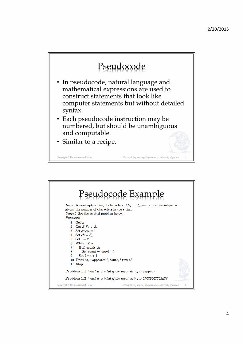
2/20/2015

4


Pseudocode

• In pseudocode, natural language and mathematical expressions are used to construct statements that look like computer statements but without detailed syntax.

• Each pseudocode instruction may be numbered, but should be unambiguous and computable.

• Similar to a recipe.

7


Pseudocode Example

8

2/20/2015

5



During and After Programming

• Make sure to provide effective documentation along with the program. This can be accomplished using:– Proper selection of variable names to reflect

the quantities they represent.

– Using comments within the program.

• Debugging a program is the process of finding and removing the “bugs” or errors in a program.

2/20/2015

6


Bugs

Bugs usually fall into one of two categories:1. Syntax errors: such as omitting a parenthesis or

comma, or spelling a command name incorrectly. MATLAB usually detects the more obvious errors and displays a message describing the error and its location.

2. Errors due to an incorrect mathematical procedure. These are called runtime errors. They do not necessarily occur every time the program is executed; their occurrence often depends on the particular input data. A common example is division by zero.

11


Finding Bugs: Debugging

To locate runtime errors, try the following:

1. Always test your program with a simple version of the problem, whose answers can be checked by hand calculations.

2. Display any intermediate calculations by removing semicolons at the end of statements.

12

2/20/2015

7


Operator Meaning

< Less than.

<= Less than or equal to.

> Greater than.

>= Greater than or equal to.

== Equal to.

~= Not equal to.

Relational Operators

13


Examples

>> x = [6 3 9];

>> y = [14 2 9];

>> z = (x < y)

z =

1 0 0

>> z = x ~= y

z =

1 1 0

>> z = x > 8

z =

0 0 1

>> a = 3;

>> b = 4;

>> a == b

ans =

0

>> a ~= b

ans =

1

>> a < b

ans =

1

>> b >= -4

ans =

1

14

2/20/2015

8


Relational operators can be used for array addressing.

For example

>> x = [6,3,9];

>> y = [14,2,9];

>> x<y

ans =

1 0 0

>> z = x(x<y)

z =

6

finds all the elements in x that are less than the corresponding elements in y. The result is z = 6.

15


The arithmetic operators +, -, *, /, and \ have precedence

over the relational operators. Thus the statement

z = 5 > 2 + 7

is equivalent to

z = 5 > (2+7)

and returns the result z = 0.

We can use parentheses to change the order of precedence; for example, z = (5 > 2) + 7 evaluates

to z = 8.

16

2/20/2015

9


The logical Class

When the relational operators are used, such as

x = (5 > 2)

they create a logical variable, in this case, x.

Logical variables may have only the values 1 (true)

and 0 (false).

17


Just because an array contains only 0s and 1s, however, it

is not necessarily a logical array. For example, in the following session k and w appear the same, but k is a

logical array and w is a numeric array, and thus an error

message is issued.

>>x = -2:2;

>>k = (abs(x)>1)

k =

1 0 0 0 1

>>z = x(k)

z =

-2 2

>>w = [1,0,0,0,1]; v = x(w)

??? Subscript indices must either be real

positive... integers or logicals.

18

2/20/2015

10


Accessing Arrays Using Logical Arrays

When a logical array is used to address another array,

it extracts from that array the elements in the

locations where the logical array has 1s.

So typing A(B), where B is a logical array of the

same size as A, returns the values of A at the indices

where B is 1.

Given A =[5,6,7;8,9,10;11,12,13] and B =

logical(eye(3)), we can extract the diagonal

elements of A by typing C = A(B) to obtain C =

[5;9;13].

See our earlier discussion of logical indexing.

19


Operator Name Definition

~ NOT ~A returns an array the same dimension as A; the new array has ones where A is zero and zeros where A is

nonzero.

& AND A & B returns an array the same dimension as A and B; the new array has ones where both A and B have nonzero elements and zeros where either A or B is zero.

| OR A | B returns an array the same dimension as A and B; the new array has ones where at least one element in A or B is nonzero and zeros where A and B are both zero.

&& Short-Circuit AND Short-circuiting means the second operand (right

hand side) is evaluated only when the result is not fully determined by the first operand (left hand side)A & B (A and B are evaluated)A && B (B is only evaluated if A is true)

|| Short-Circuit OR | can operate on arrays but || only operates on scalars

Logical Operators

20

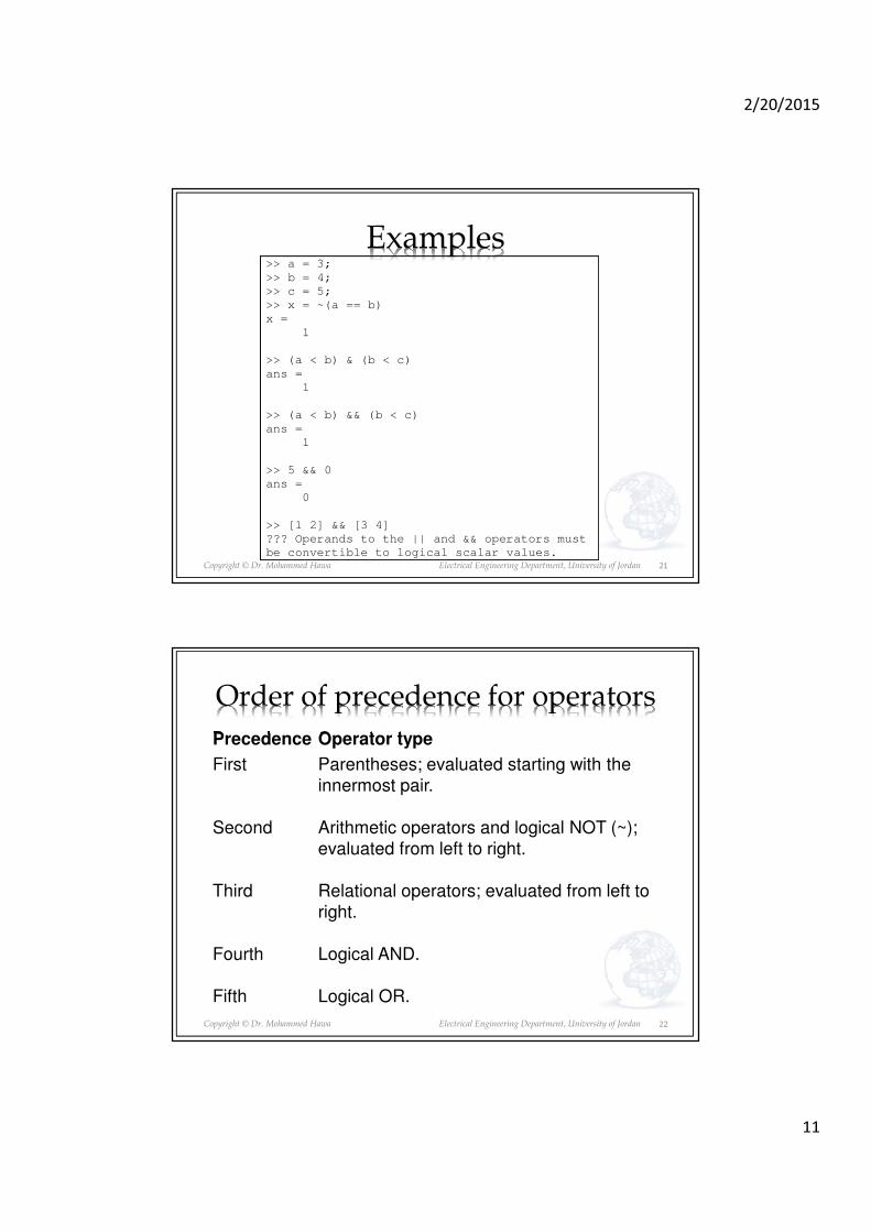
2/20/2015

11


Examples>> a = 3;

>> b = 4;

>> c = 5;

>> x = ~(a == b)

x =

1

>> (a < b) & (b < c)

ans =

1

>> (a < b) && (b < c)

ans =

1

>> 5 && 0

ans =

0

>> [1 2] && [3 4]

??? Operands to the || and && operators must

be convertible to logical scalar values.

21


Precedence Operator type

First Parentheses; evaluated starting with the

innermost pair.

Second Arithmetic operators and logical NOT (~);

evaluated from left to right.

Third Relational operators; evaluated from left to

right.

Fourth Logical AND.

Fifth Logical OR.

Order of precedence for operators

22

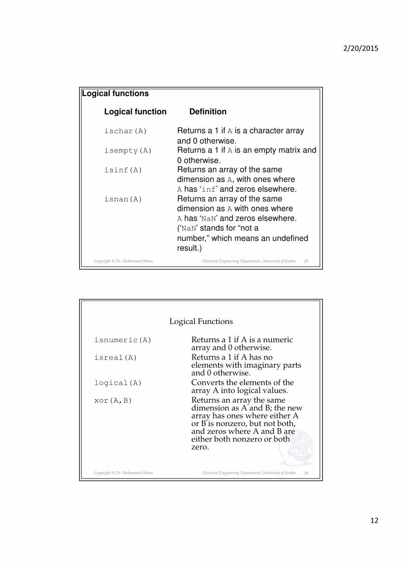
2/20/2015

12


Logical function Definition

ischar(A) Returns a 1 if A is a character array

and 0 otherwise.isempty(A) Returns a 1 if A is an empty matrix and

0 otherwise.isinf(A) Returns an array of the same

dimension as A, with ones where

A has ‘inf’ and zeros elsewhere.

isnan(A) Returns an array of the same

dimension as A with ones where

A has ‘NaN’ and zeros elsewhere.

(‘NaN’ stands for “not a

number,” which means an undefined

result.)

Logical functions

23


Logical Functions

isnumeric(A) Returns a 1 if A is a numeric array and 0 otherwise.

isreal(A) Returns a 1 if A has no elements with imaginary parts and 0 otherwise.

logical(A) Converts the elements of the array A into logical values.

xor(A,B) Returns an array the same dimension as A and B; the new array has ones where either A or B is nonzero, but not both, and zeros where A and B are either both nonzero or bothzero.

24

2/20/2015

13


Logical Operators and the find Function

Consider the session

>> x = [5, -3, 0, 0, 8];

>> y = [2, 4, 0, 5, 7];

>> x&y

ans =

1 1 0 0 1

>> z = find(x&y)

z =

1 2 5

Note that the find function returns the indices, and

not the values.

25


Conditional Statements: The if Statement

The if statement’s basic form is

if logical expression

statementsend

Every if statement must have an accompanying end

statement. The end statement marks the end of the

statements that are to be executed if the logical

expression is true.

26

2/20/2015

14


The else Statement

The basic structure for the use of the else statement is

if logical expression

statement group 1else

statement group 2end

When the test, if logical expression, is performed, where

the logical expression may be an array,

the test returns a value of true only if all the elements of

the logical expression are true!

27


The elseif Statement

The general form of the if statement is

if logical expression 1

statement group 1

elseif logical expression 2

statement group 2

else

statement group 3

end

The else and elseif statements may be omitted if not

required. However, if both are used, the else statement

must come after the elseif statement to take care of all

conditions that might be unaccounted for.

28

2/20/2015

15


Exercise

File: test.m

a = 5;

b = 4;

if a == b

disp(a);

disp(b);

elseif a < b

disp(a);

else

disp(b);

end

Matlab command prompt

>> test

4

>>

29


Example

function y = test(x)

if x >= 9

y = 15*sqrt(4*x) + 10

elseif x >= 0 % already less than 9

y = 10*x + 10

else

y = 10

end

• Suppose that we want to compute y, which is given by the equation:

30

2/20/2015

16


Example: if we fail to recognize how the test works, the

following statements do not perform the way we might

expect.

x = [4 -9 25];

if x < 0

disp(’Cant find square root of negative.’)

else

y = sqrt(x)

end

When this program is run it gives the result

y =

2 0 + 3.000i 5

31


Instead, consider what happens if we test for x positive.

x = [4, -9, 25];

if x >= 0

y = sqrt(x)

else

disp(’Cant find square root of negative.’)

end

When executed, it produces the following message:

Cant find square root of negative.

The test if x < 0 is false, and the test if x >= 0 also

returns a false value because x >= 0 returns the vector [1,0,1].

32

2/20/2015

17


Loops

• Often in your programs you will want to “loop”– repeat some commands multiple times

• If you know how many times you want to loop– use a for loop

• If you want to loop until something happens (a condition is satisfied)– use a while loop

• If you find yourself typing similar lines more than a couple of times, use a loop

33


for Loops

A simple example of a for loop is:

m = 0;

x(1) = 10;

for k = 2:3:11;

m = m + 1;

x(m+1) = x(m) + k^2;

end

k takes on the values 2, 5, 8, 11. The variable m

indicates the index of the array x. When the loop

is finished the array x will have the values

x(1)=14, x(2)=39, x(3)=103, x(4)=224.

34

2/20/2015

18


Note the following rules when using for loops with the loop variable expression k = m:s:n:

· The step value s may be negative.

Example: k = 10:-2:4 produces k = 10, 8, 6, 4.

· If s is omitted, the step value defaults to 1.

· If s is positive, the loop will not be executed if m is greater

than n.

· If s is negative, the loop will not be executed if m is less

than n.

· If m equals n, the loop will be executed only once.

· If the step value s is not an integer, round-off errors can

cause the loop to execute a different number of

passes than intended.

35


Exercise

File: loop.m

for i = 1:1:5

disp(i)

end


>> loop

1

2

3

4

5

>>

36

2/20/2015

19


Strings and Conditional Statements

A string is a variable that contains characters. Strings are

useful for creating input prompts and messages and for

storing and operating on data such as names and

addresses.

To create a string variable, enclose the characters in single

quotes. For example, the string variable name is created as

follows:

>>name = ’Mohammed Ali’

name =

Mohammed Ali

37


The following string, number, is not the same as the

variable number created by typing number = 123.

>>number = ’123’

number =

123

38

2/20/2015

20


The following prompt program is a script file that allows the user to answer Yes by typing either Y or y or by pressing the

Enter key. Any other response is treated as a No answer.

response = input(’Continue? Y/N [Y]: ’,’s’);

if (isempty(response))|(response ==

’Y’)|(response == ’y’)

response = ’Y’

else

response = ’N’

end

39


Programming Exercise #1

• Write a MATLAB program that does the following:

• The program asks you to enter your name.• It waits for you to enter your name and hit

Enter.• The program reads your name, counts its

characters and any blank spaces in the name, then displays something like this:

• You name is “Mohammed Ali”. It has 11 characters and 1 blank space.

2/20/2015

21


Using loops is slower than arrays in MATLAB

We can use the mask technique to compute the square root of only those elements of A that are no less than 0 and add

50 to those elements that are negative. The program is

A = [0, -1, 4; 9, -14, 25; -34, 49, 64];

C = (A >= 0);

A(C) = sqrt(A(C))

A(~C) = A(~C) + 50

41


while Loops

The while loop is used when the looping process

terminates because a specified condition is satisfied, and

thus the number of passes is not known in advance.

A simple example of a while loop is

x = 5;

while x < 25

disp(x)

x = 2*x - 1;

end

The results displayed by the disp statement are 5, 9, 17.

42

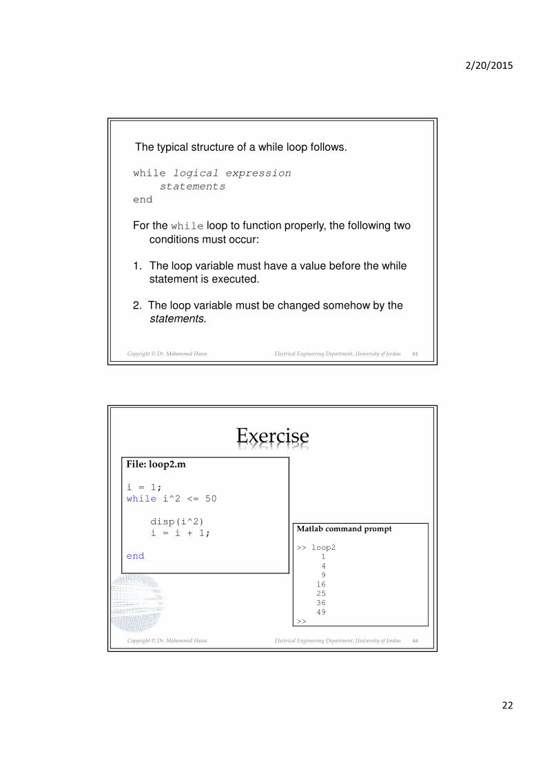
2/20/2015

22


The typical structure of a while loop follows.

while logical expression

statements

end

For the while loop to function properly, the following two

conditions must occur:

1. The loop variable must have a value before the while

statement is executed.

2. The loop variable must be changed somehow by the

statements.

43


ExerciseFile: loop2.m

i = 1;

while i^2 <= 50

disp(i^2)

i = i + 1;

end


>> loop2

1

4

9

16

25

36

49

>>

44

2/20/2015

23


Editor/Debugger containing program to be analyzed

45


The break statement

• break terminates the execution of a loop, so if you have a nested loop, break will only quit the innermost loop, and the program will continue running.

s=6; % initialize s to 6

while s~=1 % as long as s is not equal to 1 stay in loop

if s==17 % if s equals 17

sprintf('Found 17 in the loop!!')

break;

end

if mod(s,2) % the actual "brains" of the iteration

s=s/2;

else

s=3*s+1;

end

end

46

2/20/2015

24


The continue statement

The following code uses a continue statement to avoid

computing the logarithm of a negative number.

x = [10,1000,-10,100];

y = NaN*x;

for k = 1:length(x)

if x(k) < 0

continue

end

y(k) = log10(x(k));

end

y

The result is y = [1 3 NaN 2].

47


Homework

• Write a script file to determine how many terms are required for the sum of the series 5��– 2�, � � 1, 2, 3, … to exceed 10,000. What is the sum for this many terms?

total = 0; k = 0;

while total < 1e4

k = k + 1;

total = total + 5*k^2 - 2*k;

end

disp(’The number of terms is:’)

disp(k)

disp(’The sum is:’)

disp(total)

• The sum is 10,203 after 18 terms.

48

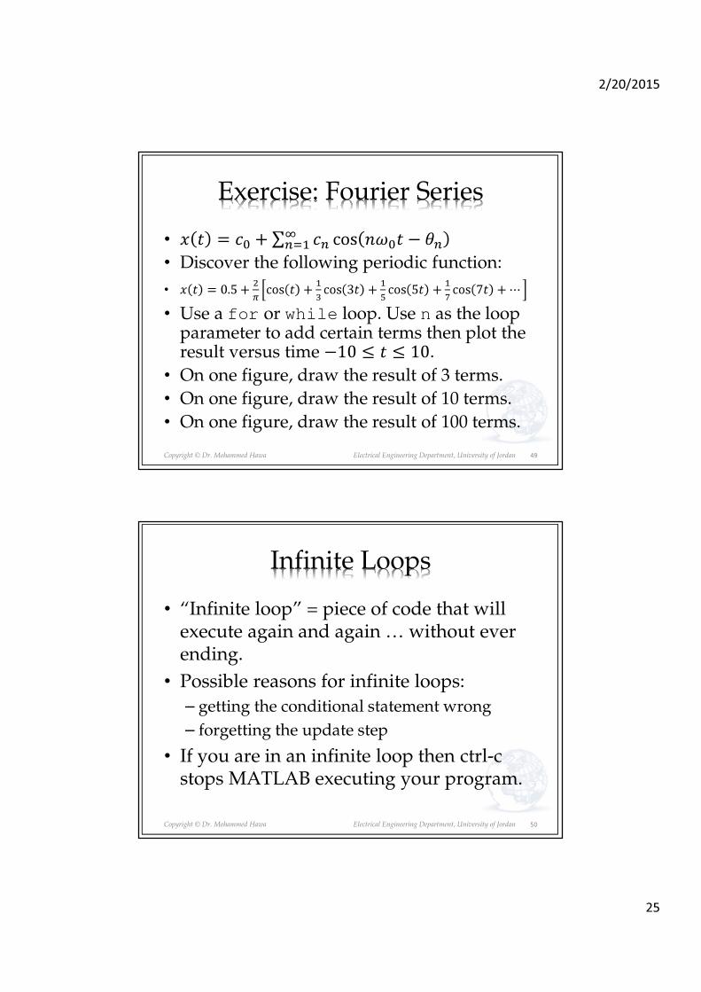
2/20/2015

25


Exercise: Fourier Series

• � � � �� ∑ �� cos ��

��

• Discover the following periodic function:

• � � 0.5 ��

�cos � �

�

�cos 3� �

�

�cos 5� �

�

�cos 7� �⋯

• Use a for or while loop. Use n as the loop parameter to add certain terms then plot the result versus time �10 � � � 10.

• On one figure, draw the result of 3 terms.



49


Infinite Loops

• “Infinite loop” = piece of code that will execute again and again … without ever ending.

• Possible reasons for infinite loops:

– getting the conditional statement wrong

– forgetting the update step

• If you are in an infinite loop then ctrl-c stops MATLAB executing your program.

50

2/20/2015

26


The switch statement

The switch statement provides an alternative to using the

if, elseif, and else commands.

Anything programmed using switch can also be

programmed using if statements.

However, for some applications the switch statement is

more readable than code using the if structure.

51


Syntax of switch

switch input expression (can be a scalar or string).case value1

statement group 1

case value2

statement group 2

.

.

.

otherwise

statement group n

end

52

2/20/2015

27


The following switch block displays the point on the

compass that corresponds to that angle.

switch angle

case 45

disp(’Northeast’)

case 135

disp(’Southeast’)

case 225

disp(’Southwest’)

case 315

disp(’Northwest’)

otherwise

disp(’Direction Unknown’)

end

53


Boolean Variables

• MATLAB allows boolean variables that take true/false values

if (atUniversity & stillAStudent)

needMoreMoney = true;

end

54

2/20/2015

28



• Write a MATLAB program to solve this:

• One investment opportunity pays 5.5% annual profit, while a second investment opportunity pays 4.5% annual profit.

• Determine how much longer it will take to accumulate at least $50,000 in the second investment opportunity compared to the first if you invest $1000 initially and $1000 at the end of each year.

55



• Write a MATLAB program that asks you for a hexadecimal integer number.

• The program should read that number and convert it to decimal.

• Example: 84CD hexadecimal is 33997 decimal.

• Can you improve on your program so it accepts binary or hexadecimal or decimal and converts it to all other formats? You need to accept numbers written in something like this: 94CAh or 110110001b.

56

2/20/2015

29


Homework



• 4.2, 4.4, 4.5, 4.11, 4.13, 4.15, 4.16, 4.17, 4.23, 4.24, 4.25, 4.26, 4.33, 4.37, 4.39, 4.47

57

2/20/2015

1

Lecture 6: Plottingin MATLAB





A picture is worth a thousand words

• MATLAB allows you to plot data sets for better visualization and interpretation.

• There are different types of plots available in MATLAB (see next) including 2D and 3D plots.

• You can control all aspects of the plot: lines, colors, grids, labels, etc.

• Plotting clear and easy-to-read figures is an important skill, which you gain from experience.

• For pointers, read in your textbook the Requirements for a Correct Plot (Table 5.1-1, page 221), and Hints for Improving Plots (Table 5.1-3, page 226).

2

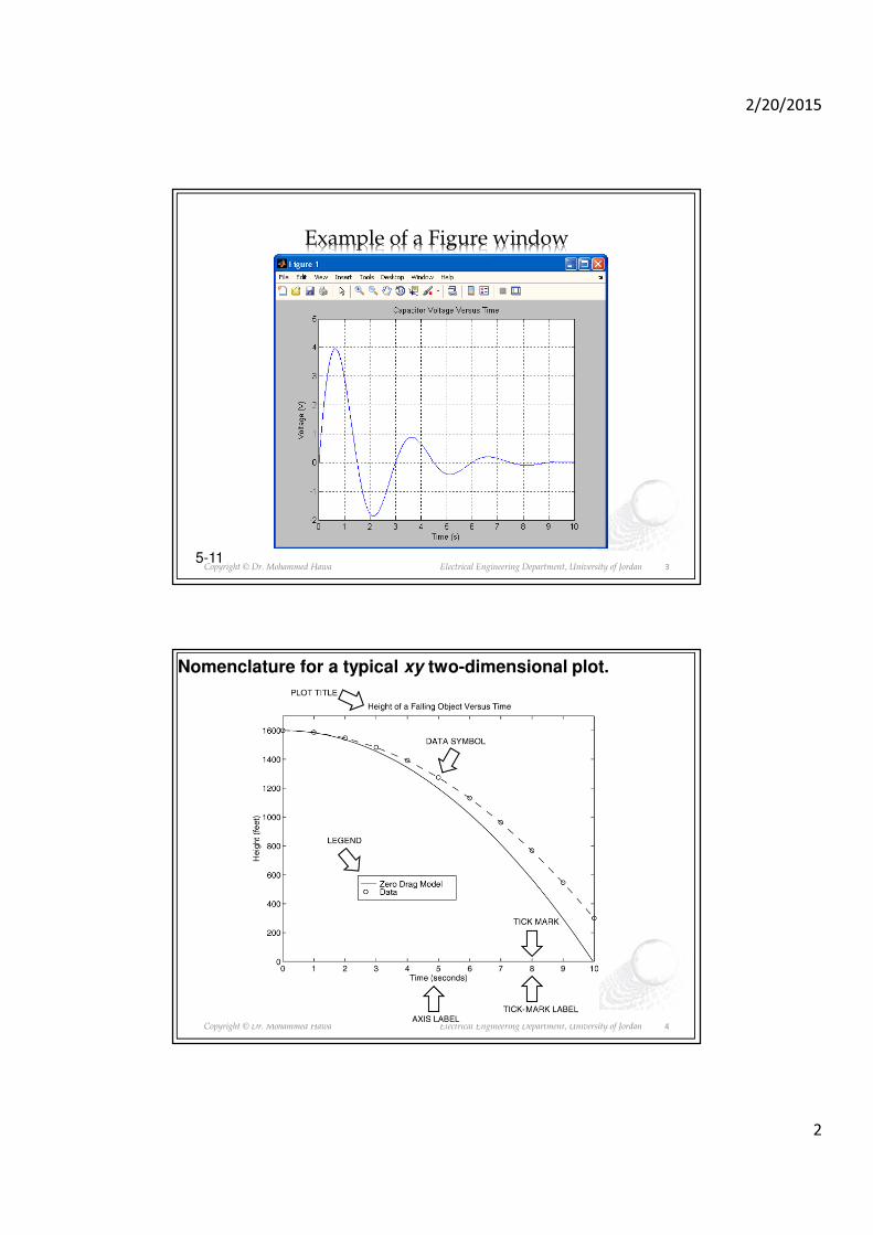
2/20/2015

2


Example of a Figure window

5-113


Nomenclature for a typical xy two-dimensional plot.

4

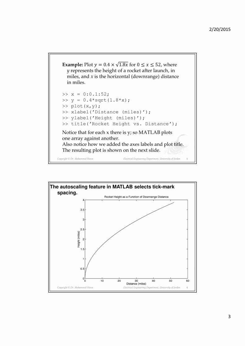
2/20/2015

3


Example: Plot � = 0.4 × 1.8� for 0 ≤ � ≤ 52, where y represents the height of a rocket after launch, in miles, and x is the horizontal (downrange) distance in miles.

>> x = 0:0.1:52;

>> y = 0.4*sqrt(1.8*x);

>> plot(x,y);

>> xlabel(’Distance (miles)’);

>> ylabel(’Height (miles)’);

>> title(’Rocket Height vs. Distance’);

Notice that for each x there is y; so MATLAB plotsone array against another.Also notice how we added the axes labels and plot title.The resulting plot is shown on the next slide.

5


The autoscaling feature in MATLAB selects tick-mark spacing.

6

2/20/2015

4


The plot will appear in the Figure window. You can use the

plot in other applications in several ways:

1. You can print a hard copy of the figure by selecting

File | Print menu item in the Figure window.

2. You can save the plot to a file to be used later. You can

save the plot by selecting File | Save As menu item.

Possible file formats include: *.fig (MATLAB format),

*.bmp, *.eps, *.jpg, *.png, *.tif, *.pdf, …. Another way

to save is File | Export Setup that allows specifying

options for the output file, then selecting Export.

3. You can copy a figure to the clipboard and then paste it

into another application using the Edit | Copy Figure

menu item. For options, use Edit | Copying Options

menu item.

7


When you have finished with the plot, close the figure

window by selecting File | Close menu item in the

figure window.

If you do not close the window, it will not re-appear

when a new plot command is executed. However,

the figure will still be updated.

8

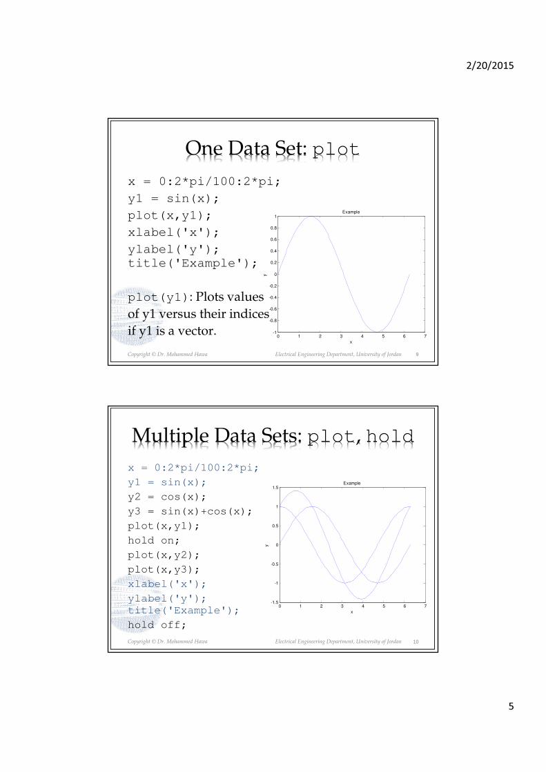
2/20/2015

5


One Data Set: plot

x = 0:2*pi/100:2*pi;

y1 = sin(x);

plot(x,y1);

xlabel('x');

ylabel('y');

title('Example');

plot(y1): Plots values

of y1 versus their indices

if y1 is a vector. 0 1 2 3 4 5 6 7

-1

-0.8

-0.6

-0.4

-0.2

0

0.2

0.4

0.6

0.8

1

x

y

Example

9


Multiple Data Sets: plot, hold

x = 0:2*pi/100:2*pi;

y1 = sin(x);

y2 = cos(x);

y3 = sin(x)+cos(x);

plot(x,y1);

hold on;

plot(x,y2);

plot(x,y3);

xlabel('x');

ylabel('y');

title('Example');

hold off;

0 1 2 3 4 5 6 7-1.5

-1

-0.5

0

0.5

1

1.5

x

y

Example

10

2/20/2015

6


Or better use one plot command

x = 0:2*pi/100:2*pi;

y1 = sin(x);

y2 = cos(x);

y3 = sin(x)+cos(x);

plot(x,y1,x,y2,x,y3);

xlabel('x');

ylabel('y');

title('Example');

% Notice the auto coloring

% by MATLAB

0 1 2 3 4 5 6 7-1.5

-1

-0.5

0

0.5

1

1.5

x

y

Example

11


Colors, Data Markers & Line Types

• You can also specify your own line styles in the plot command.

• For full details enter help plot in MATLAB.

12

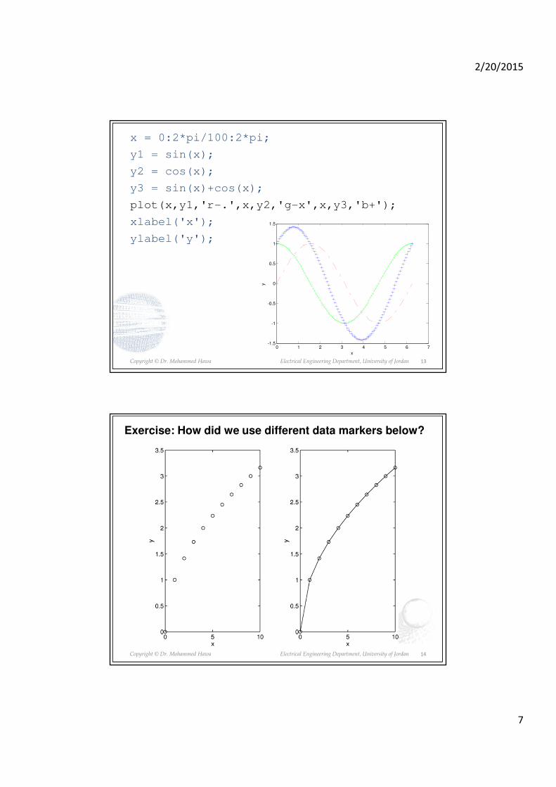
2/20/2015

7


x = 0:2*pi/100:2*pi;

y1 = sin(x);

y2 = cos(x);

y3 = sin(x)+cos(x);

plot(x,y1,'r-.',x,y2,'g-x',x,y3,'b+');

xlabel('x');

ylabel('y');

0 1 2 3 4 5 6 7-1.5

-1

-0.5

0

0.5

1

1.5

x

y

13


Exercise: How did we use different data markers below?

14

2/20/2015

8


Legends• With multiple lines on the same plot it is a good idea to add a legend.

legend('sin','cos','sin + cos');

legend('sin','cos','sin+cos','Location','North');

• You can also move the legend with the mouse.

0 1 2 3 4 5 6 7-1.5

-1

-0.5

0

0.5

1

1.5

x

y

sin

cos

sin + cos

0 1 2 3 4 5 6 7-1.5

-1

-0.5

0

0.5

1

1.5

x

y

sin

cos

sin + cos

15


Labeling Curves and Data

The legend command automatically obtains from the

plot the line type used for each data set and displays a

sample of this line type in the legend box next to the

string you selected. The following script file produced

the plot in the next slide.

x = 0:0.01:2;

y = sinh(x);

z = tanh(x);

plot(x,y,x,z,'--');

legend('sinh(x)', 'tanh(x)');

gtext(‘text’): Places a string in the Figure

window at a point specified by the mouse.

text(x,y,’text’): Places a string in the Figure

window at a point specified by coordinates x, y.

16

2/20/2015

9


Application of the legend command.

I moved the legend to an empty space using the mouse.

0 0.2 0.4 0.6 0.8 1 1.2 1.4 1.6 1.8 20

0.5

1

1.5

2

2.5

3

3.5

4

sinh(x)

tanh(x)

17


The grid and axis Commands

MATLAB will automatically determine the maximum and

minimum values for the axes. You can use the axis

command to override the MATLAB selections for the axis

limits. The syntax is axis([xmin xmax ymin ymax]).

This command sets the scaling for the x- and y-axes to the

minimum and maximum values indicated.

The grid command displays gridlines at the tick marks

corresponding to the tick labels. Type grid on to add

gridlines; type grid off to stop plotting gridlines. When

used by itself, grid toggles this feature on or off, but you

might want to use grid on and grid off to be sure.

18

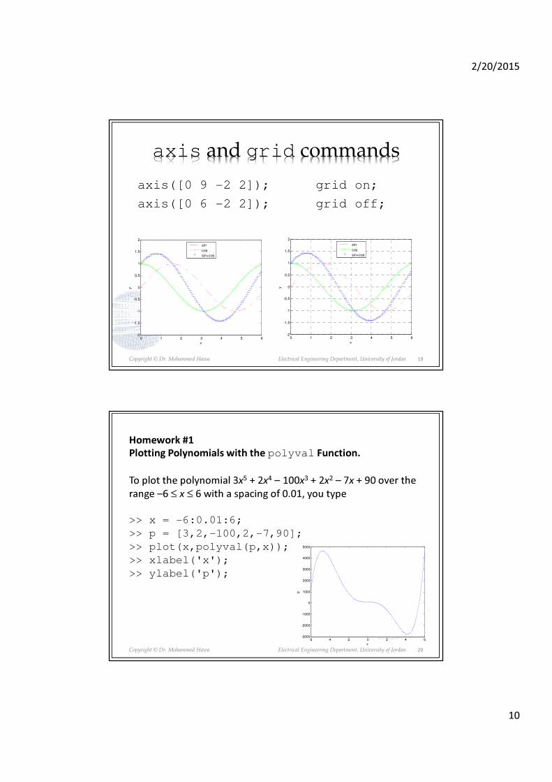
2/20/2015

10


axis and grid commands

axis([0 9 -2 2]);

axis([0 6 -2 2]);

0 1 2 3 4 5 6-2

-1.5

-1

-0.5

0

0.5

1

1.5

2

x

y

sin

cos

sin+cos

0 1 2 3 4 5 6-2

-1.5

-1

-0.5

0

0.5

1

1.5

2

x

y

sin

cos

sin+cos

grid on;

grid off;

19


Homework #1

Plotting Polynomials with the polyval Function.

To plot the polynomial 3x5 + 2x4 – 100x3 + 2x2 – 7x + 90 over the

range –6 ≤ x ≤ 6 with a spacing of 0.01, you type

>> x = -6:0.01:6;

>> p = [3,2,-100,2,-7,90];

>> plot(x,polyval(p,x));

>> xlabel('x');

>> ylabel('p');

-6 -4 -2 0 2 4 6-3000

-2000

-1000

0

1000

2000

3000

4000

5000

x

p

20

2/20/2015

11


Homework #2

• The polyfit function is based on the least-squares method. It fits a polynomial of degree n to data described by the vectors x and y, where x is the independent variable.

• Syntax: p = polyfit(x,y,n)• It returns a row vector p of length n+1 that

contains the polynomial coefficients in order of descending powers.

• For the following census data, draw the actual points and the best 5th order polynomial fit for such data.

21


year = 1810:10:2010;

population = 1e6*[3.9 5.3 7.2 9.6 12.9 17.1 23.1 31.4 38.6 50.2 62.9 76. 92. 105.7 122.8 131.7 150.7 179. 205. 226.5 248.7];

coeff = polyfit(year, population, 5)

f = polyval(coeff, year);

plot(year, population, 'bo', year, f, 'r--');

1800 1850 1900 1950 2000 20500

0.5

1

1.5

2

2.5

3x 10

8

22

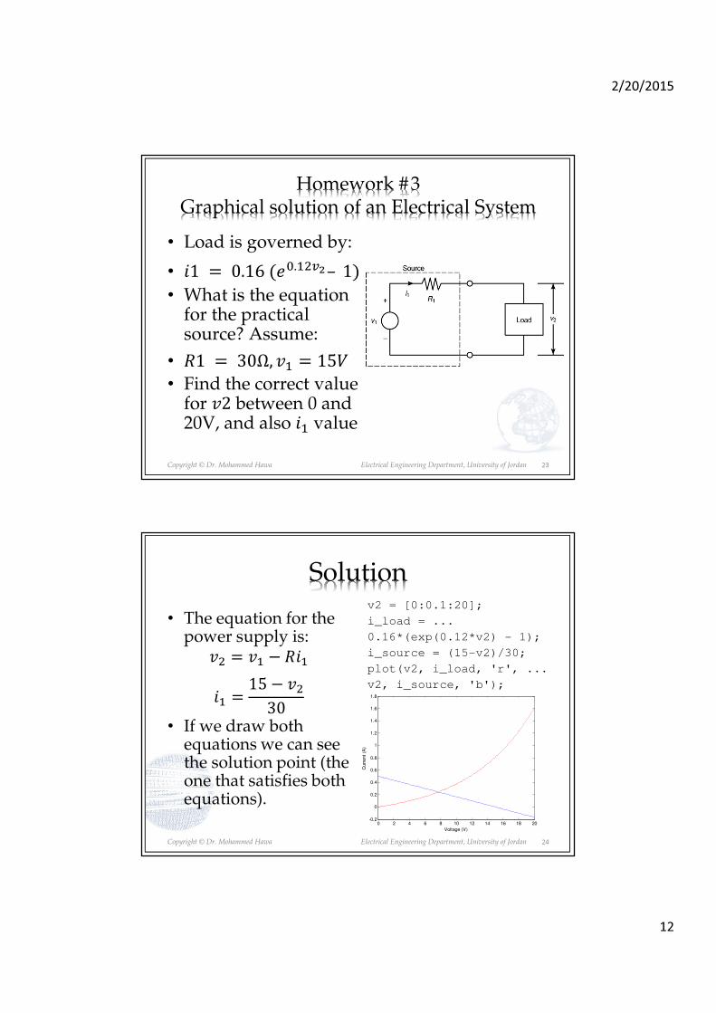
2/20/2015

12


Homework #3Graphical solution of an Electrical System

• Load is governed by:

• �1 � 0.16��.��– 1

• What is the equation for the practical source? Assume:

• �1 � 30Ω, �� 15�

• Find the correct value for �2 between 0 and 20V, and also �� value

23


Solutionv2 = [0:0.1:20];

i_load = ...

0.16*(exp(0.12*v2) - 1);

i_source = (15-v2)/30;

plot(v2, i_load, 'r', ...

v2, i_source, 'b');

• The equation for the power supply is:

��

�� 15 � ��

30

• If we draw both equations we can see the solution point (the one that satisfies both equations).

0 2 4 6 8 10 12 14 16 18 20-0.2

0

0.2

0.4

0.6

0.8

1

1.2

1.4

1.6

1.8

Voltage (V)

Curr

ent

(A)

24

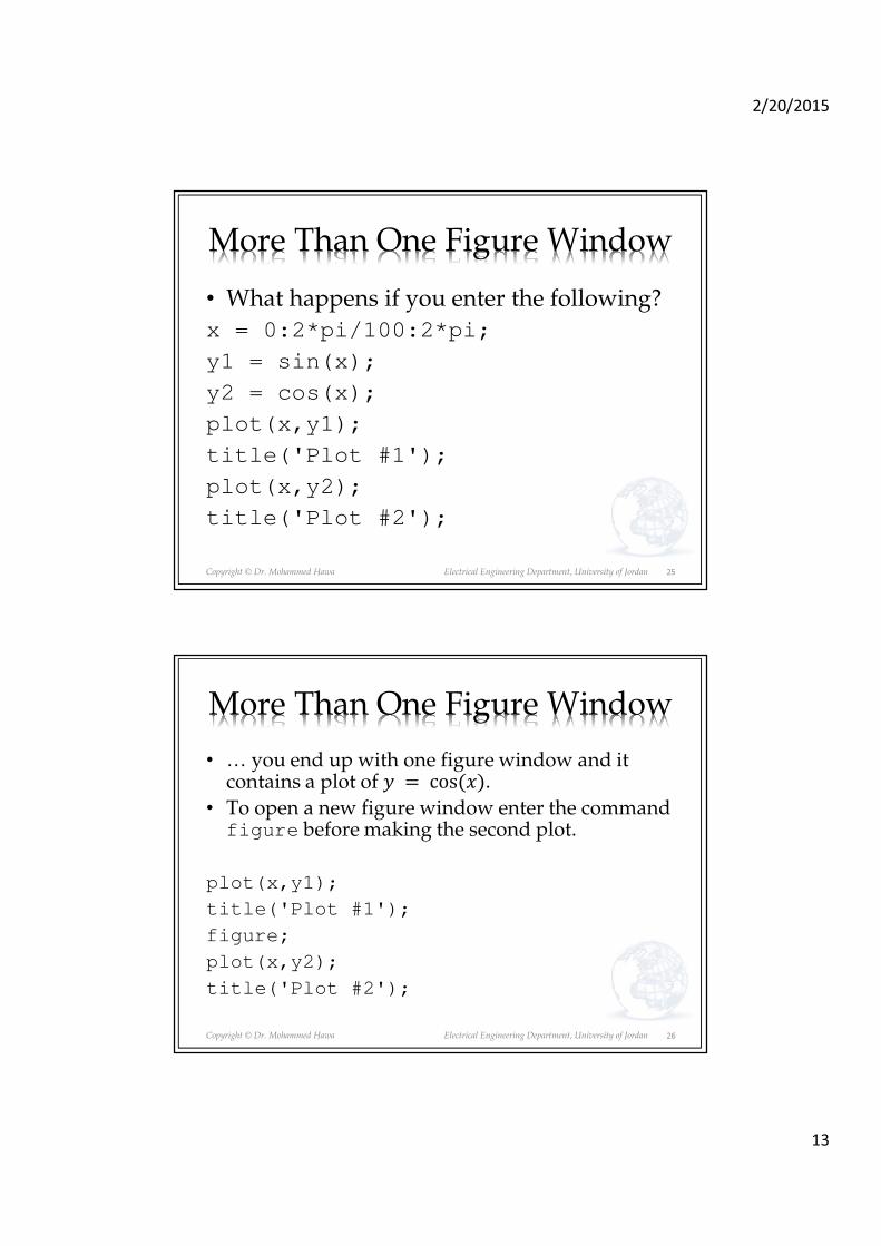
2/20/2015

13


More Than One Figure Window

• What happens if you enter the following?

x = 0:2*pi/100:2*pi;

y1 = sin(x);

y2 = cos(x);

plot(x,y1);

title('Plot #1');

plot(x,y2);

title('Plot #2');

25


More Than One Figure Window

• … you end up with one figure window and it contains a plot of � � cos��.

• To open a new figure window enter the command figure before making the second plot.

plot(x,y1);

title('Plot #1');

figure;

plot(x,y2);

title('Plot #2');

26

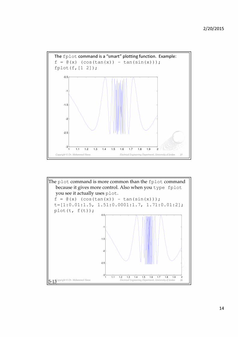
2/20/2015

14


The fplot command is a “smart” plotting function. Example:

f = @(x) (cos(tan(x)) - tan(sin(x)));

fplot(f,[1 2]);

1 1.1 1.2 1.3 1.4 1.5 1.6 1.7 1.8 1.9 2-3

-2.5

-2

-1.5

-1

-0.5

27


The plot command is more common than the fplot command because it gives more control. Also when you type fplotyou see it actually uses plot.f = @(x) (cos(tan(x)) - tan(sin(x)));

t=[1:0.01:1.5, 1.51:0.0001:1.7, 1.71:0.01:2];

plot(t, f(t));

5-131 1.1 1.2 1.3 1.4 1.5 1.6 1.7 1.8 1.9 2

-3

-2.5

-2

-1.5

-1

-0.5

28

2/20/2015

15


Complex Plot: Real vs. Imaginary

n = [0:0.01:10];

y = (0.1+0.9j).^n;

plot(y);

xlabel('Real');

ylabel('Imaginary');

• Similar to: plot(real(y),imag(y)); -1 -0.8 -0.6 -0.4 -0.2 0 0.2 0.4 0.6 0.8 1

-0.8

-0.6

-0.4

-0.2

0

0.2

0.4

0.6

0.8

1

Real

Imagin

ary

29


Subplots

You can use the subplot command to obtain several

smaller “subplots” in the same figure. The syntax is

subplot(m,n,p). This command divides the Figure

window into an array of rectangular panes with m rows and

n columns. The variable p tells MATLAB to place the output

of the plot command following the subplot command

into the pth pane.

For example, subplot(3,2,5) creates an array of six

panes, three panes deep and two panes across, and directs

the next plot to appear in the fifth pane (in the bottom-left

corner).

30

2/20/2015

16


Subplots

• subplot(m,n,p)

31


Examplex = 0:2*pi/100:2*pi;

y1 = sin(x);

y2 = cos(x);

y3 = sin(x)+cos(x);

subplot(2,2,1);

plot(x,y1,'r-.');

title('sin(x)');

subplot(2,2,2);

plot(x,y2,'go');

title('cos(x)');

subplot(2,2,3);

plot(x,y3,'b+');

title('sin(x)+cos(x)');

0 2 4 6 8-1

-0.5

0

0.5

1sin(x)

0 2 4 6 8-1

-0.5

0

0.5

1cos(x)

0 2 4 6 8-2

-1

0

1

2sin(x)+cos(x)

32

2/20/2015

17


Homework:

The following script file shows two plots of the functions

y = e−1.2x sin(10x + 5) for 0 ≤ x ≤ 5

and y = |x3 − 100| for −6 ≤ x ≤ 6.

x = 0:0.01:5;

y = exp(-1.2*x).*sin(10*x+5);

subplot(1,2,1);

plot(x,y);

axis([0 5 -1 1]);

x = -6:0.01:6;

y = abs(x.^3-100);

subplot(1,2,2);

plot(x,y);

axis([-6 6 0 350])The figure is shown

on the next slide.

33


Application of the subplot command.

0 1 2 3 4 5-1

-0.8

-0.6

-0.4

-0.2

0

0.2

0.4

0.6

0.8

1

-5 0 50

50

100

150

200

250

300

350

34

2/20/2015

18


Log-scale Plots• Why use log scales? Linear scales cannot properly

display wide variations in data values. • MATLAB has three commands. The appropriate

command depends on which axis you want to be a log scale.

• loglog(x,y): both scales logarithmic.• semilogx(x,y): x-axis is logarithmic and y-axis is

rectilinear.• semilogy(x,y): y-axis is logarithmic and x-axis is

rectilinear.• The syntax is similar to the plot command.

35


x = [0.1:0.01:100];

y = sqrt((100*(1-0.01*x.^2).^2 ...

+0.02*x.^2) ...

./ ((1-x.^2).^2+0.1*x.^2));

plot(x,y);

0 10 20 30 40 50 60 70 80 90 1000

5

10

15

20

25

30

35

36

2/20/2015

19


x = [0.1:0.01:100];

y = sqrt((100*(1-0.01*x.^2).^2 ...

+0.02*x.^2) ...

./ ((1-x.^2).^2+0.1*x.^2));

loglog(x,y);

10-2

10-1

100

101

102

10-2

10-1

100

101

102

37


Logarithmic Plots

It is important to remember the following points when

using log scales:

1. You cannot plot negative numbers on a log scale,

because the logarithm of a negative number is not

defined as a real number.

2. You cannot plot the number 0 on a log scale, because

log10 0 = ln 0 = −∞. You must choose an appropriately

small number as the lower limit on the plot.

(continued…)38

2/20/2015

20


3. The tick-mark labels on a log scale are the actual values

being plotted; they are not the logarithms of the

numbers. For example, the range of x values in the plot

in the above Figure is from 10−2 = 0.01 to 102 = 100.

4. Gridlines and tick marks within a decade are unevenly

spaced. If 8 gridlines or tick marks occur within the

decade, they correspond to values equal to 2, 3, 4, . . . ,

8, 9 times the value represented by the first gridline or

tick mark of the decade.

Logarithmic Plots (continued)

(continued…)39


5. Equal distances on a log scale correspond to

multiplication by the same constant (as opposed to

addition of the same constant on a rectilinear scale).

For example, all numbers that differ by a factor of 10 are

separated by the same distance on a log scale. That is,

the distance between 0.3 and 3 is the same as the

distance between 30 and 300. This separation is

referred to as a decade or cycle.

The plot shown in the above Figure covers four decades in

x (from 0.01 to 100) and four decades in y.

Logarithmic Plots (continued)

40

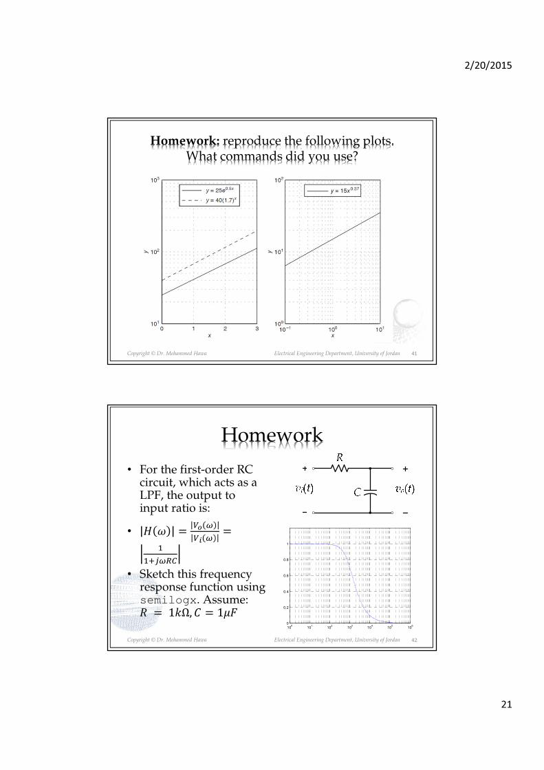
2/20/2015

21


Homework: reproduce the following plots. What commands did you use?

41


Homework

• For the first-order RC circuit, which acts as a LPF, the output to input ratio is:

• � � ��

��

�

��

• Sketch this frequency response function using semilogx. Assume: � � 1�Ω, � 1��

100

101

102

103

104

105

106

0

0.2

0.4

0.6

0.8

1

42

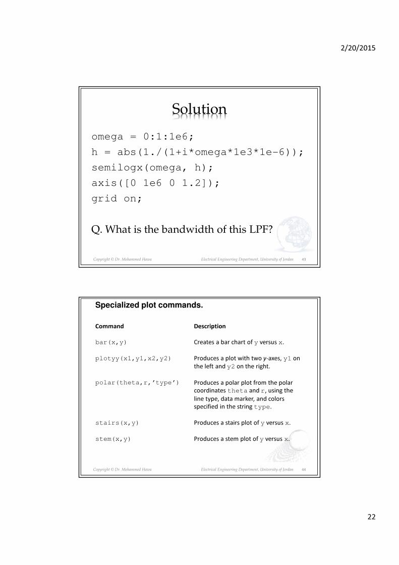
2/20/2015

22


Solution

omega = 0:1:1e6;

h = abs(1./(1+i*omega*1e3*1e-6));

semilogx(omega, h);

axis([0 1e6 0 1.2]);

grid on;

Q. What is the bandwidth of this LPF?

43


Command

bar(x,y)

plotyy(x1,y1,x2,y2)

polar(theta,r,’type’)

stairs(x,y)

stem(x,y)

Description

Creates a bar chart of y versus x.

Produces a plot with two y-axes, y1 on

the left and y2 on the right.

Produces a polar plot from the polar

coordinates theta and r, using the

line type, data marker, and colors

specified in the string type.

Produces a stairs plot of y versus x.

Produces a stem plot of y versus x.

Specialized plot commands.

44

2/20/2015

23


x = [0:pi/20:pi];

bar(x,sin(x));

-0.5 0 0.5 1 1.5 2 2.5 3 3.50

0.1

0.2

0.3

0.4

0.5

0.6

0.7

0.8

0.9

1

45


theta = [0:pi/90:2*pi];

polar(theta , sin(2*theta));

grid;

0.2

0.4

0.6

0.8

1

30

210

60

240

90

270

120

300

150

330

180 0

46

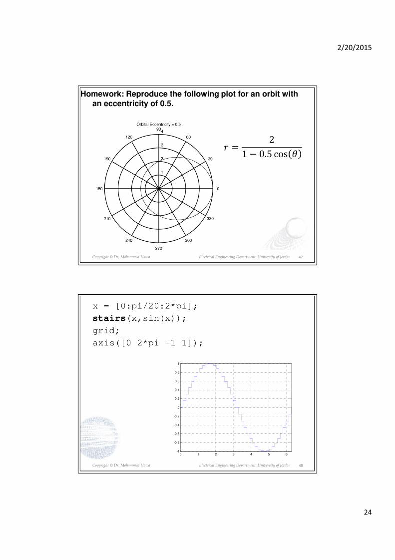
2/20/2015

24


Homework: Reproduce the following plot for an orbit with an eccentricity of 0.5.

� =2

1 − 0.5 cos �

47


x = [0:pi/20:2*pi];

stairs(x,sin(x));

grid;

axis([0 2*pi -1 1]);

0 1 2 3 4 5 6-1

-0.8

-0.6

-0.4

-0.2

0

0.2

0.4

0.6

0.8

1

48

2/20/2015

25


x = [-2*pi:pi/20:2*pi];

x = x + (~x)*eps;

y = sin(pi*x)./(pi*x);

stem(x,y);

axis([-2*pi 2*pi -.25 1]);

-6 -4 -2 0 2 4 6

-0.2

0

0.2

0.4

0.6

0.8

49


x = [-2*pi:pi/20:4*pi];

fill(x,sin(x),'c');

axis([0 4*pi -1 1]);

0 2 4 6 8 10 12-1

-0.8

-0.6

-0.4

-0.2

0

0.2

0.4

0.6

0.8

1

50

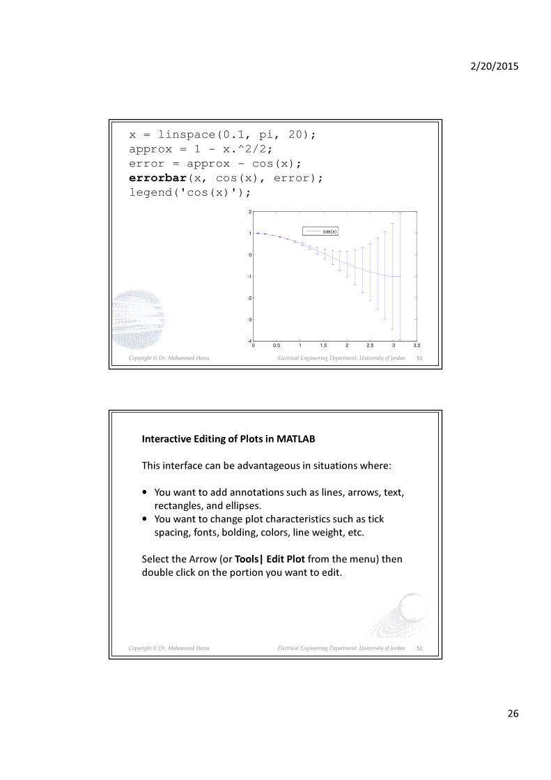
2/20/2015

26


x = linspace(0.1, pi, 20);

approx = 1 - x.^2/2;

error = approx - cos(x);

errorbar(x, cos(x), error);

legend('cos(x)');

0 0.5 1 1.5 2 2.5 3 3.5-4

-3

-2

-1

0

1

2

cos(x)

51


Interactive Editing of Plots in MATLAB

This interface can be advantageous in situations where:

• You want to add annotations such as lines, arrows, text,

rectangles, and ellipses.

• You want to change plot characteristics such as tick

spacing, fonts, bolding, colors, line weight, etc.

Select the Arrow (or Tools| Edit Plot from the menu) then

double click on the portion you want to edit.

52

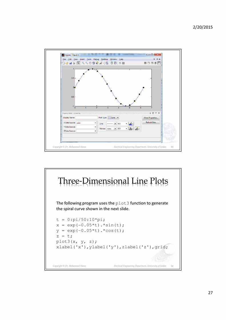
2/20/2015

27



The following program uses the plot3 function to generate

the spiral curve shown in the next slide.

t = 0:pi/50:10*pi;

x = exp(-0.05*t).*sin(t);

y = exp(-0.05*t).*cos(t);

z = t;

plot3(x, y, z);

xlabel('x'),ylabel('y'),zlabel('z'),grid;

Three-Dimensional Line Plots

54

2/20/2015

28


The curve x = = = = e−−−−0.05t sin t, y = = = = e−−−−0.05t cos t, z = = = = t plotted with the plot3 function.

-1

-0.5

0

0.5

1

-1

-0.5

0

0.5

10

5

10

15

20

25

30

35

xy

z

55


The following session shows how to generate the surface plot of

the function z = xe−[(x−y2)2+y2], for −2 ≤ x ≤ 2 and −2 ≤ y ≤ 2, with a

spacing of 0.1. This plot appears in the next slide.

[X,Y] = meshgrid(-2:0.1:2);

Z = X.*exp(-((X-Y.^2).^2+Y.^2));

mesh(X,Y,Z);

xlabel('x'),ylabel('y'),zlabel('z');

[X,Y] = meshgrid(-2:0.1:2);

Z = X.*exp(-((X-Y.^2).^2+Y.^2));

surf(X,Y,Z);

xlabel('x'),ylabel('y'),zlabel('z'),colorbar

Surface Plots: mesh and surf

56

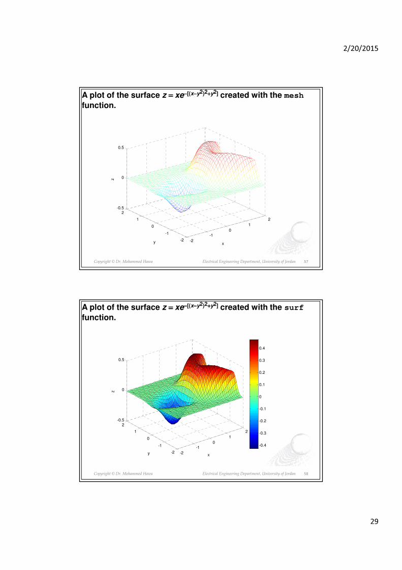
2/20/2015

29


A plot of the surface z = = = = xe−−−−[(x−−−−y2)2++++y2] created with the mesh

function.

-2

-1

0

1

2

-2

-1

0

1

2-0.5

0

0.5

xy

z

57


A plot of the surface z = = = = xe−−−−[(x−−−−y2)2++++y2] created with the surf

function.

-2

-1

0

1

2

-2

-1

0

1

2-0.5

0

0.5

xy

z

-0.4

-0.3

-0.2

-0.1

0

0.1

0.2

0.3

0.4

58

2/20/2015

30


The following session generates the contour plot of the

function whose surface plot is shown above;

namely, z = xe−[(x−y2)2+y2], for −2 ≤ x ≤ 2 and −2 ≤ y ≤ 2, with a

spacing of 0.1. This plot appears in the next slide.

[X,Y] = meshgrid(-2:0.1:2);

Z = X.*exp(-((X-Y.^2).^2+Y.^2));

[cs, h] = contour(X,Y,Z);

xlabel('x'),ylabel('y'),zlabel('z');

clabel(cs, h, 'labelspacing', 72);

59


A contour plot of the surface z = = = = xe−−−−[(x−−−−y2)2++++y2] created with the contour function.

-2

-1

0

1

2

-2

-1

0

1

2-0.5

0

0.5

xy

z

-0.4

-0.3

-0.3

-0.3

-0.2

-0.2

-0.2

-0.2

-0.2

-0.1

-0.1-0.1

-0.1

-0.1-0.1

-0.1

00

00

0

0.1

0.1

0.1

0.1

0.1

0.1

0.10.1

0.1

0.1

0.2

0.2

0.2

0.2

0.2

0.2

0.2

0.2

0.2

0.2

0.3

0.3

0.3

0. 3

0.3

0.30.3

0.3

0.3

0.3

0.3

0.4

0.4

0.4

0.40.4

0.40.4

0.4

0.4

x

y

-2 -1.5 -1 -0.5 0 0.5 1 1.5 2-2

-1.5

-1

-0.5

0

0.5

1

1.5

2

60

2/20/2015

31


Contours are useful for Terrain

61


Vector fields: quiver

• quiver draws little arrows to indicate a gradient or other vector field.

• Although it produces a 2-D plot, it is often used in conjunction with contour. As an example, consider the scalar function of two variables: � � �� .

• The gradient of � is defined as the vector

field: ��

��,��

�� 2�, 1

62

2/20/2015

32


quiver

• The following statements draw arrows indicating the direction of the vector �� at points in the x-y plane (see next slide).

[x y] = meshgrid(-2:0.2:2, -2:0.2:2);

V = x.^2 + y;

dx = 2*x;

dy = ones(size(dx)); % dy same size as dx

quiver(x, y, dx, dy);

hold on;

contour(x, y, V);

hold off;

63


quiver alone; and with contour

-2.5 -2 -1.5 -1 -0.5 0 0.5 1 1.5 2 2.5-2

-1.5

-1

-0.5

0

0.5

1

1.5

2

2.5

-2.5 -2 -1.5 -1 -0.5 0 0.5 1 1.5 2 2.5-2

-1.5

-1

-0.5

0

0.5

1

1.5

2

2.5

64

2/20/2015

33


Useful for Electromagnetic Fields

65


Homework% What is the output of this MATLAB code? Use help if you need.

figure;

t = linspace(0, 2*pi, 512);

[u,v] = meshgrid(t) ;

a = -0.2 ; b = .5 ; c = .1 ;

x = (a*(1-v/(2*pi)) .* (1+cos(u)) + c) .* cos(2*v);

y = (a*(1-v/(2*pi)) .* (1+cos(u)) + c) .* sin(2*v);

z = b*v/(2*pi) + a*(1-v/(2*pi)) .* sin(u);

surf(x,y,z,y);

shading interp;

axis off;

axis equal;

colormap(hsv(1024));

material shiny;

lighting gouraud;

lightangle(80, -40);

lightangle(-90, 60);

view([-150 10]);

66

2/20/2015

34


Animation and Movies!

• A movies is just successive plots seen in quick succession.

• We can plot data repeatedly on a single figure.

• For example the function � � sin��

x = 0:2*pi/100:2*pi;

for t = 0:0.05:5 % 5 seconds

y = sin(x+t);

plot(x,y,’k’)

pause(0.2); % 200 ms between frames

end

67


Homework: Creating Movies

• To create a movie a sequence of frames are “grabbed” from the figure, stored in an array and written out as .avi file.

nFrame = 1; % frame counter

x = 0:2*pi/100:2*pi;

for t=0:0.05:5

y=sin(x+t);

plot(x,y);

pause(0.2);

movie(nFrame) = getframe; % grab frame & store it

nFrame = nFrame + 1;

end

movie2avi(movie,'animation.avi'); % save movie

68

2/20/2015

35


Homework



• Solve: 5.3, 5.5, 5.9, 5.11, 5.15, 5.20, 5.27, 5.29, 5.35, 5.36, 5.39.

69

3/30/2015

1

Lecture 8: Calculus and Differential Equations





Numerical Methods

• MATLAB provides many functions that support numerical solutions to common math problems:– Integration and Differentiation (Calculus)– Finding zeros of a function– Solving ordinary differential equations– Many others

• Numerical analysis provides answers as numbers, not closed-form solutions as in analytical solutions (see next lecture for symbolic math in MATLAB).

2

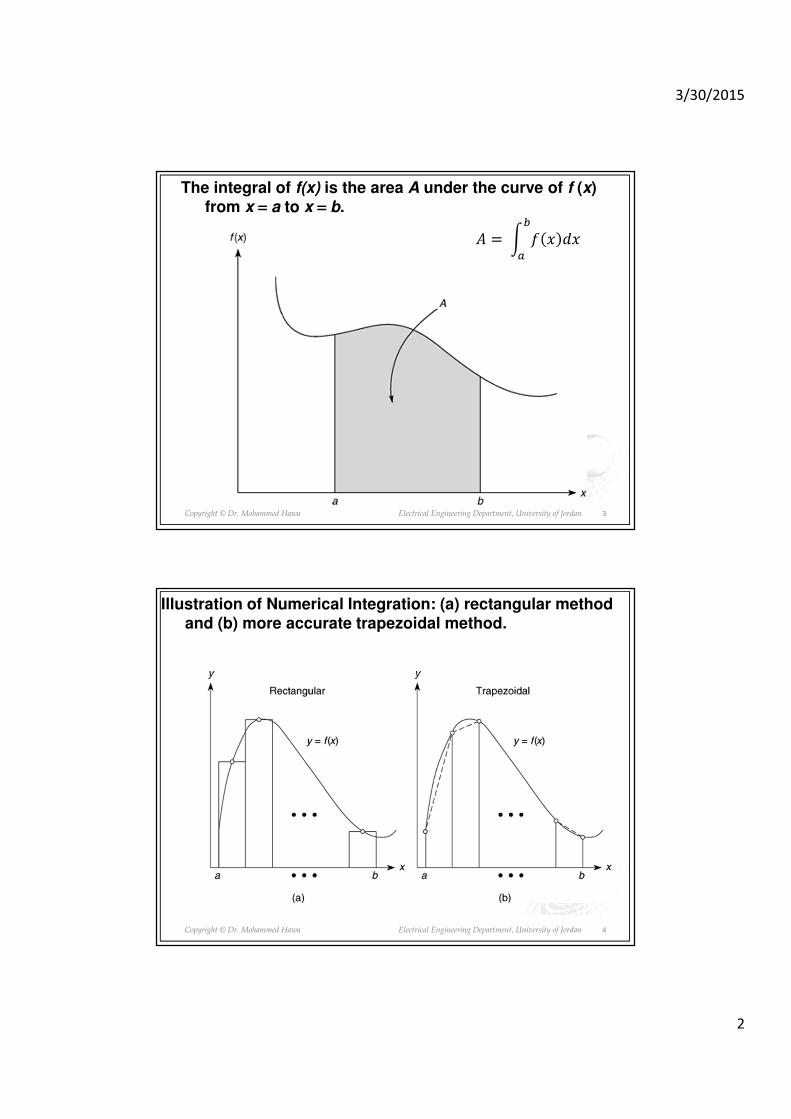
3/30/2015

2


The integral of f(x) is the area A under the curve of f (x)

from x ==== a to x ==== b.

� = � � � ��

�

3


Illustration of Numerical Integration: (a) rectangular method and (b) more accurate trapezoidal method.

4

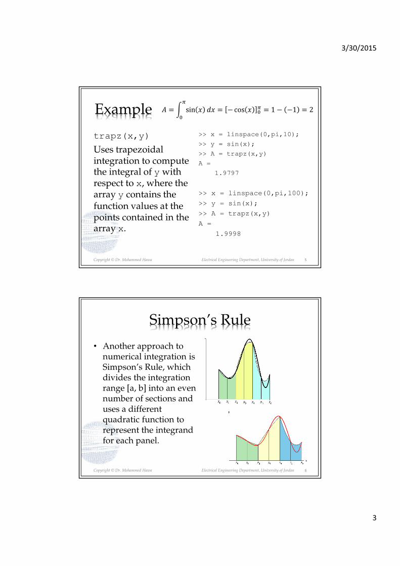
3/30/2015

3


Example

>> x = linspace(0,pi,10);

>> y = sin(x);

>> A = trapz(x,y)

A =

1.9797

>> x = linspace(0,pi,100);

>> y = sin(x);

>> A = trapz(x,y)

A =

1.9998

trapz(x,y)

Uses trapezoidal integration to compute the integral of y with respect to x, where the array y contains the function values at the points contained in the array x.

� � � sin � ��

�

� cos � �

� � 1 1 � 2

5


Simpson’s Rule

• Another approach to numerical integration is Simpson’s Rule, which divides the integration range [a, b] into an even number of sections and uses a different quadratic function to represent the integrand for each panel.

6

3/30/2015

4


quad(fun, a, b)

quad(fun, a, b, tol)

quadl(fun,a,b)

dblquad(fun, a, b, c, d)

triplequad(fun,a,b,c,d,e,f)

Uses an adaptive Simpson’s rule to compute

the integral of the function whose handle is

fun, with a the lower limit and b the upper

limit. The function fun must accept a vector

argument. The parameter tol is optional, and

indicates the specified error tolerance.

Uses Lobatto quadrature to compute the

integral of the function fun. The rest of the

syntax is identical to quad.

computes the integral of f(x,y) from x = a to b,

and y = c to d. The function fun must accept a

vector argument x and scalar y, and it must

return a vector result.

computes the integral of f(x,y,z) from x = a to

b, y = c to d, and z = e to f. The function must

accept a vector x, and scalar y and z.

Important numerical integration functions:

7


Although the quad and quadl functions are

more accurate than trapz, they are restricted to

computing the integrals of functions and cannot be

used when the integrand is specified by a set of

points. For such cases, use the trapz function.

8

3/30/2015

5


MATLAB function quad implements an adaptive

version of Simpson’s rule, while the quadl function is

based on an adaptive Lobatto integration algorithm.

To compute the integral of sin(x) from 0 to π, type

>> A = quad(@sin,0,pi)

The answer given by MATLAB is 2.0000, which is correct.

We use quadl the same way; namely,

>> A = quadl(@sin,0,pi).

9


To integrate cos(x2 ) from 0 to 2�, create the function in

an m-file:

function yy = cossq(x)

yy = cos(x.^2);

Note that we must use array exponentiation. Then quad

function is called as follows:

>> quad(@cossq, 0, sqrt(2*pi))

ans =

0.6119

Or you can use an anonymous function:

>> f = @(x)(1./(x.^3 - 2*x - 5));

>> quad(f, 0, 2)

ans =

-0.4605 0 0.2 0.4 0.6 0.8 1 1.2 1.4 1.6 1.8 2-1.5

-1

-0.5

0

0 0.5 1 1.5 2 2.5-1.5

-1

-0.5

0

0.5

1

1.5

10

3/30/2015

6


A = dblquad(fun, a, b, c, d) computes the integral of f(x,y)

from x = a to b, and y = c to d. Example: f(x,y) = xy2.

>> fun = @(x,y) x.*y^2;

>> A = dblquad(fun, 1, 3, 0, 1)

A =

1.3333

A = triplequad(fun, a, b, c, d, e, f) computes the

triple integral of f(x,y, z) from x = a to b, y = c to d, and z = e to f.

Example: f(x,y,z) = (xy -y2)/z.

>> fun = @(x,y,z)(x*y - y^2)/z;

>> A = triplequad(fun, 1,3, 0,2, 1,2)

A =

1.8484

Note: The function must accept a vector x, but scalar y and z.

Double and Triple Integrals

�� , � ��

�

�

�

�� , �, � ��

�

�

�

�

�

11


Be careful: function singularity

>> f = @(x) ( 1./(x-1));

>> quad(f, 0, 2)

Warning: Infinite or Not-

a-Number function value

encountered.

> In quad at 113

ans =

NaN

0 0.2 0.4 0.6 0.8 1 1.2 1.4 1.6 1.8 2-100

-80

-60

-40

-20

0

20

40

60

80

100

� 11 � ��

�

�

12

3/30/2015

7


Numerical differentiation: Illustration of estimating the

derivative dy////dx.

�� lim

∆�→�

∆�∆�

��

��

13


MATLAB provides the diff function to use for computing

derivative estimates.

d = diff(y), where y is a vector of n elements, the

result is a vector d containing n − 1 elements that are the

differences between adjacent elements in y. That is:

d=[y(2)-y(1), y(3)-y(2),..., y(n)-y(n-1)]

For example:

>> y = [5, 7, 12, -20];

>> diff(y)

ans =

2 5 -32

14

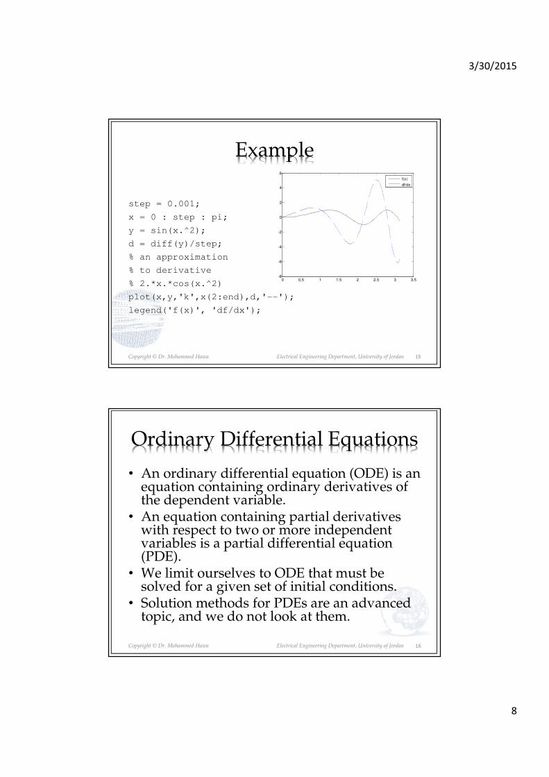
3/30/2015

8


Example

step = 0.001;

x = 0 : step : pi;

y = sin(x.^2);

d = diff(y)/step;

% an approximation

% to derivative

% 2.*x.*cos(x.^2)

plot(x,y,'k',x(2:end),d,'--');

legend('f(x)', 'df/dx');

0 0.5 1 1.5 2 2.5 3 3.5-8

-6

-4

-2

0

2

4

6

f(x)

df/dx

15


Ordinary Differential Equations

• An ordinary differential equation (ODE) is an equation containing ordinary derivatives of the dependent variable.

• An equation containing partial derivatives with respect to two or more independent variables is a partial differential equation (PDE).

• We limit ourselves to ODE that must be solved for a given set of initial conditions.

• Solution methods for PDEs are an advanced topic, and we do not look at them.

16

3/30/2015

9


Several Methods

• Several numerical methods to solve ODEs.• Examples include:

– Euler and Backward Euler methods– Predictor-Corrector method– First-order exponential integrator method– Runge-Kutta methods– Adams-Moulton methods– Gauss-Radau methods– Adams-Bashforth methods– Hermite–Obreschkoff methods– Fehlberg methods– Parker–Sochacki methods– Nyström methods– Quantized State Systems methods

17


Multiple Solvers

• MATLAB offers multiple ODE solvers, each uses different methods.

• Ode23: Solves non-stiff differential equations, low order method.

• ode45: Solves non-stiff differential equations, medium order method: uses a combination of fourth- and fifth-order Runge-Kutta methods.

• ode23s: Solves stiff differential equations, low order method.

• ode15i: Solves fully implicit differential equations, variable order method.

• And so on.• We will limit ourselves to the ode45 solver.

18

3/30/2015

10


Example: Find the response of the first-order RC circuit .

� �� + � = 0

� 0 = �(�. . )

� �� + � = �

� 0 = �(�. . )

�() = � 0 ��/(��)

� = � + (� 0 − �)��/(��)

�� =��

�� =��

19


Solving First-Order Differential Equations

First write the equation as dy/dt = f(t,y) then solve it using this syntax:

[t,y] = ode45(@f,tspan,y0)

where @f is the handle of the function file whose inputs must be t and

y, and whose output must be a column vector representing dy/dt; that

is, f(t,y). The number of rows in the output column vector must equal

the order of the equation.

The array tspan contains the starting and ending values of the

independent variable t, and optionally any intermediate values.

The array y0 contains the initial values of y. If the equation is first

order, then y0 is a scalar.

20

3/30/2015

11


The circuit model for zero input voltage � and � = 0.1 is:

0.1 ×�� + � = 0

And the i.c. is �(0) = 2 V.

First re-write the equation in the required format:

�

�= −10�

Next define the following function file. Note that the order

of the input arguments must be t and y.

f = @(t,y) -10*y;

21


The solver is called as follows, and the solution plotted along

with the analytical solution y_true. The initial condition is

�(0) = 2.

f = @(t,y) -10*y;

[t, y] = ode45(f, [0 0.5], 2);

y_analytical = 2*exp(-10*t);

plot(t,y,'o', t, y_analytical);

legend('ODE solver', 'Actual');

xlabel('Time(s)');

ylabel('Capacitor Voltage');

Note that we need not generate the array t to evaluate

y_analytical, because t is generated by the ode45

function.

The plot is shown on the next slide.

22

3/30/2015

12


Free (natural) response of an RC circuit

(decaying exponential).

0 0.05 0.1 0.15 0.2 0.25 0.3 0.35 0.4 0.45 0.50

0.2

0.4

0.6

0.8

1

1.2

1.4

1.6

1.8

2

Time(s)

Capacitor

Voltage

ODE solver

Actual

23


The circuit model for input voltage � = 10� and � = 0.1:

0.1 ×�� + � = 10

And the i.c. is �(0) = 2 V.


�� = −10� + 100



f = @(t,y) -10*y+100;

24

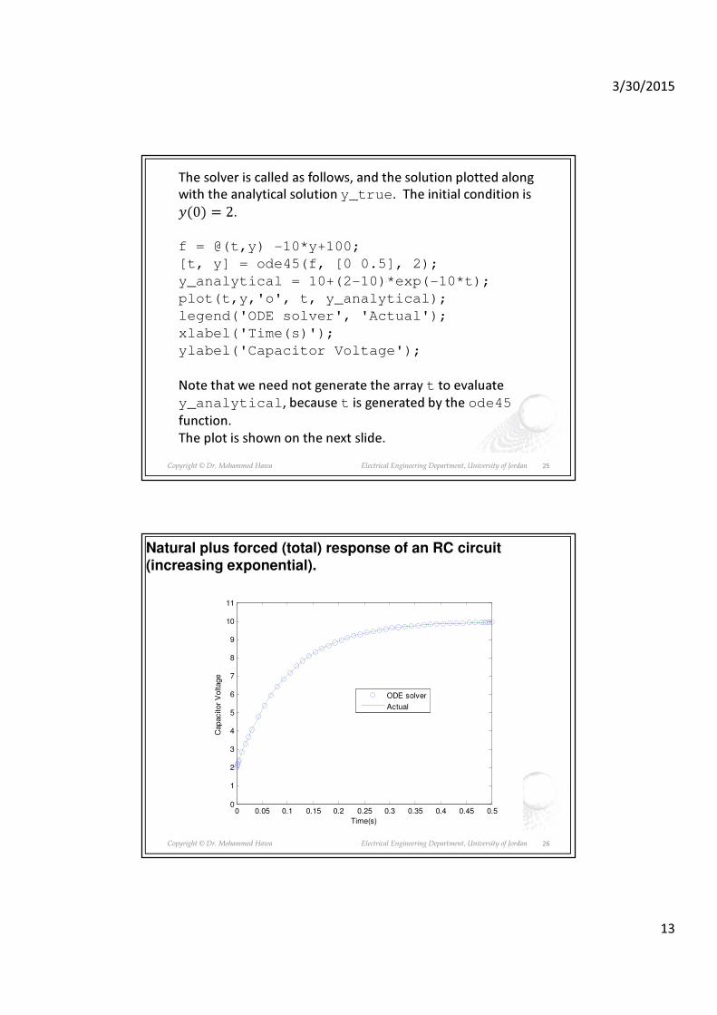
3/30/2015

13


The solver is called as follows, and the solution plotted along

with the analytical solution y_true. The initial condition is

�(0) = 2.

f = @(t,y) -10*y+100;

[t, y] = ode45(f, [0 0.5], 2);

y_analytical = 10+(2-10)*exp(-10*t);

plot(t,y,'o', t, y_analytical);

legend('ODE solver', 'Actual');

xlabel('Time(s)');

ylabel('Capacitor Voltage');

Note that we need not generate the array t to evaluate

y_analytical, because t is generated by the ode45

function.

The plot is shown on the next slide.

25


Natural plus forced (total) response of an RC circuit (increasing exponential).

0 0.05 0.1 0.15 0.2 0.25 0.3 0.35 0.4 0.45 0.50

1

2

3

4

5

6

7

8

9

10

11

Time(s)

Capacitor

Voltage

ODE solver

Actual

26

3/30/2015

14


The circuit model for input voltage � = 10� �/�.� sin ��

�.��

and � = 0.1:

0.1 ×�� + � = 10� �/�.� sin 2��

0.03

And assume the i.c. is �(0) = 0 V.


�� = −10� + 100� �/�.� sin 2��

0.03



f = @(t,y) -10*y+100* ...

exp(-1*t/0.3).*sin(2*pi*t/0.03);

27


Result

0 0.2 0.4 0.6 0.8 1 1.2-10

-5

0

5

10

Time (s)

Applie

d V

oltage

0 0.2 0.4 0.6 0.8 1 1.2-0.5

0

0.5

1

Time (s)

Capacitor

Voltage

28

3/30/2015

15


Extension to Higher-Order Equations

To use the ODE solvers to solve an equation of 2nd order or

higher, you must first write the equation as a set of first-order

equations.

Example:

5�� + 7

�� + 4� = � �

By re-arranging to get the highest derivative:

�� =

1

5� � −

4

5� −

7

5

��

29


Example (Continue)

��

��

1

5� � �

4

5� �

7

5

��

��

We then change variables: �� /��

Hence: ��/�� /��

Also: �� . Hence we have two equations:

��

��

��

��

1

5� � �

4

5��

7

5��

30

3/30/2015

16


Example (Continue)

��

��

��

��

1

5� � �

4

5��

7

5��

This form is sometimes called the Cauchy form or the state-variable form.

We now define a function that accepts two values of x and then computes the values of ��/�� and ��/�� and stores them in a column vector.

31


��

��

��

��

1

5sin �

4

5��

7

5��

d = @(t,x) [x(2); sin(t)/5-4*x(1)/5-7*x(2)/5];

[t, x] = ode45(d, [0 6], [3 9]);

Here ��0� � 3 and ��0� � 9, and we solve for 0 � � 6. Also � � sin��.Note x is a matrix with two columns. The first column contains the values of x1at the various times generated by the solver; the second column contains the values of x2.

If you type plot(t, x), you will obtain a plot of both x1 and x2 versus t. Thus, type plot(t, x(:,1)) to see the result for y.

Example (Code)

32

3/30/2015

17


Result

0 1 2 3 4 5 6-1

0

1

2

3

4

5

6

7

33


HW: Alternative Solution

Define the function in an m-file:

function xdot = d(t, x)

xdot(1) = x(2);

xdot(2) = (1/5)*(sin(t)-4*x(1)-7*x(2));

xdot = [xdot(1); xdot(2)];

Use the function to solve the ODE:

[t, x] = ode45(@d, [0 6], [3 9]);

% notice the need to use handles

plot(t, x(:,1));

34

3/30/2015

18


Homework



• Solve: 9.1, 9.4, 9.14, 9.16, 9.23, 9.27, 9.31, 9.34.

35

3/30/2015

1

Lecture 9: Symbolic Processing in MATLAB





The sym function can be used to create “symbolic objects” in

MATLAB.

If the input argument to sym is a string, the result is a symbolic

number or variable. If the input argument is a numeric scalar or

matrix, the result is a symbolic representation of the given

numeric values.

For example, typing x = sym('x') creates the symbolic

variable with name x, and typing y = sym('y') creates a

symbolic variable named y.

Typing x = sym('x', 'real') tells MATLAB to assume that

x is real. Typing x = sym('x', 'unreal') tells MATLAB to

assume that x is not real.

2

3/30/2015

2


The syms function enables you to combine more than

one such statement into a single statement.

For example, typing syms x is equivalent to typing

x = sym('x'), and typing syms x y u v creates

the four symbolic variables x, y, u, and v.

3


Symbolic vs. Numeric Objects

4

>> a = 5

a =

5

>> class(5)

ans =

double

>> b = 't'

b =

t

>> class(b)

ans =

char

>> x = sym('x')

x =

x

>> class(x)

ans =

sym

>> syms y

>> class(y)

ans =

sym

3/30/2015

3


You can use the sym function to create symbolic

constants by using a numerical value for the argument.

For example, typing

fraction = sym('1/3')

sqroot2 = sym('sqrt(2)')

pi = sym('pi')

will create symbolic constants that avoid the floating-point

approximations inherent in the values of π, 1/3, and √2.

5


You can use symbolic variables in expressions and as

arguments of functions. You use the operators

+ - * / ^ and the built-in functions just as you use

them with numerical calculations. For example, typing

>> syms x y

>> s = x + y;

>> r = sqrt(x^2 + y^2);

creates the symbolic variables s and r. The terms s =

x + y and r = sqrt(x^2 + y^2) are examples

of symbolic expressions.

Symbolic Expressions

6

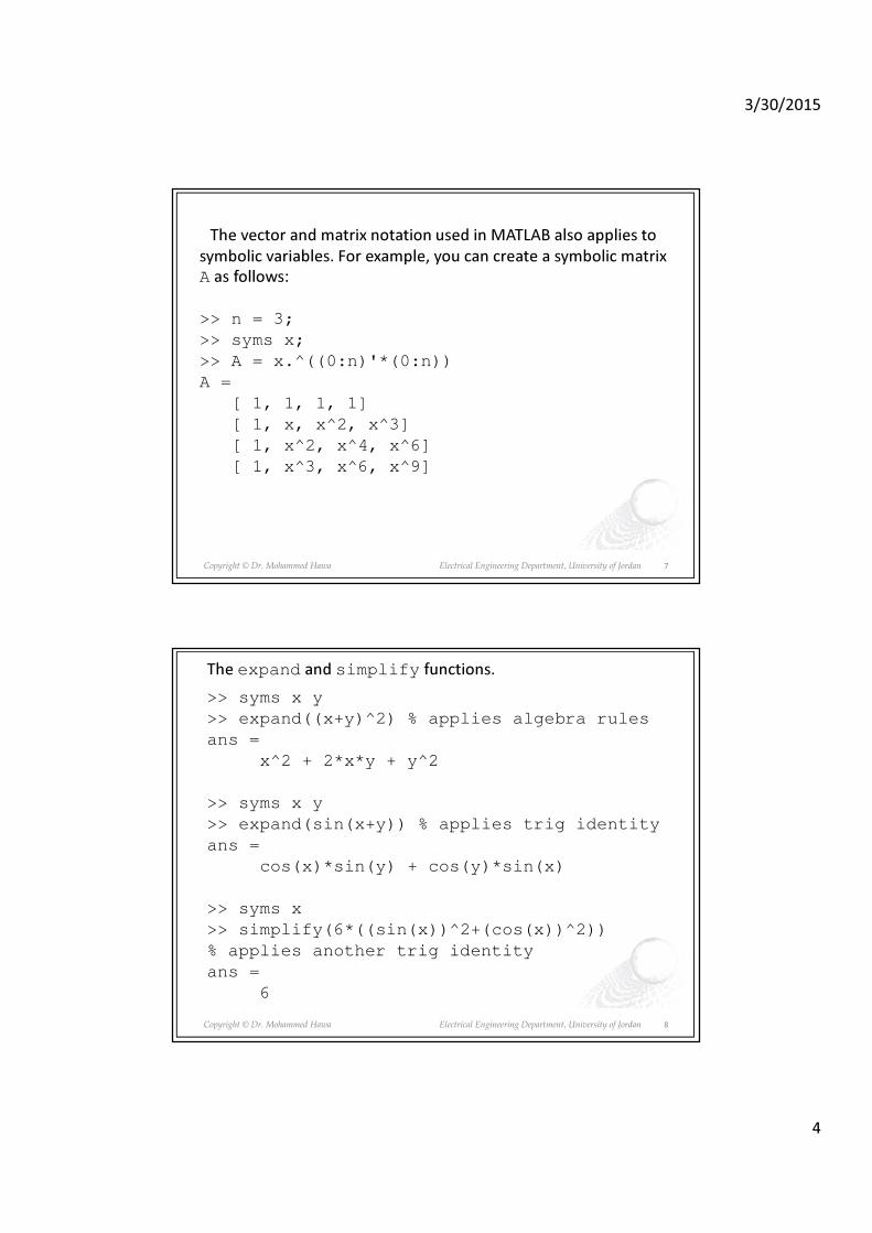
3/30/2015

4


The vector and matrix notation used in MATLAB also applies to

symbolic variables. For example, you can create a symbolic matrix

A as follows:

>> n = 3;

>> syms x;

>> A = x.^((0:n)'*(0:n))

A =

[ 1, 1, 1, 1]

[ 1, x, x^2, x^3]

[ 1, x^2, x^4, x^6]

[ 1, x^3, x^6, x^9]

7


The expand and simplify functions.

>> syms x y

>> expand((x+y)^2) % applies algebra rules

ans =

x^2 + 2*x*y + y^2

>> syms x y

>> expand(sin(x+y)) % applies trig identity

ans =

cos(x)*sin(y) + cos(y)*sin(x)

>> syms x

>> simplify(6*((sin(x))^2+(cos(x))^2))

% applies another trig identity

ans =

6

8

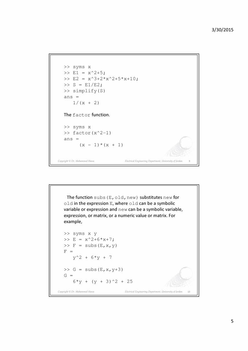
3/30/2015

5


>> syms x

>> E1 = x^2+5;

>> E2 = x^3+2*x^2+5*x+10;

>> S = E1/E2;

>> simplify(S)

ans =

1/(x + 2)

The factor function.

>> syms x

>> factor(x^2-1)

ans =

(x - 1)*(x + 1)

9


The function subs(E,old,new) substitutes new for

old in the expression E, where old can be a symbolic

variable or expression and new can be a symbolic variable,

expression, or matrix, or a numeric value or matrix. For

example,

>> syms x y

>> E = x^2+6*x+7;

>> F = subs(E,x,y)

F =

y^2 + 6*y + 7

>> G = subs(E,x,y+3)

G =

6*y + (y + 3)^2 + 25

10

3/30/2015

6


If you want to tell MATLAB that f is a function of the variable t,

type f = sym('f(t)'). Thereafter, f behaves like a function

of t, and you can manipulate it with the toolbox commands. For

example, to create a new function g(t) = f (t + 2) − f (t), the

session is

>> syms t

>> f = sym('f(t)');

>> g = subs(f,t,t+2)-f

g =

f(t+2)-f(t)

Once a specific function is defined for f(t), the function g(t) will be

available.

11


Use the subs and double functions to evaluate an expression

numerically. Use subs(E,old,new) to replace old with a

numeric value new in the expression E. The result is of class

double. For example,

>> syms x

>> E = x^2+6*x+7;

>> G = subs(E,x,2)

G =

23

>> class(G)

ans =

double

12

3/30/2015

7


The MATLAB function ezplot(E) generates a plot of a

symbolic expression E, which is a function of one variable.

The default range of the independent variable is the interval

[−2π, 2π] unless this interval contains a singularity.

The optional form ezplot(E,[xmin xmax]) generates

a plot over the range from xmin to xmax.

Example:

>> syms x

>> E = x^2 - 6*x + 7;

>> ezplot(E, [-2 6]);

13


Result

-2 -1 0 1 2 3 4 5 6

0

5

10

15

20

x

x2 - 6 x + 7

14

3/30/2015

8


Order of Precedence.

MATLAB does not always arrange expressions in a form that

we normally would use.

For example, MATLAB might provide an answer in the form

-c+b, whereas we would normally write b-c.

The order of precedence used by MATLAB must be

constantly kept in mind to avoid misinterpreting the

MATLAB output (see earlier slides).

MATLAB frequently expresses results in the form 1/a*b,

whereas we would normally write b/a.

15


The solve function.

There are three ways to use the solve function. For example,

to solve the equation x + 5 = 0, one way is

>> eq1 = 'x+5=0';

>> solve(eq1)

ans =

-5

The second way is

>> solve('x+5=0')

ans =

-5

16

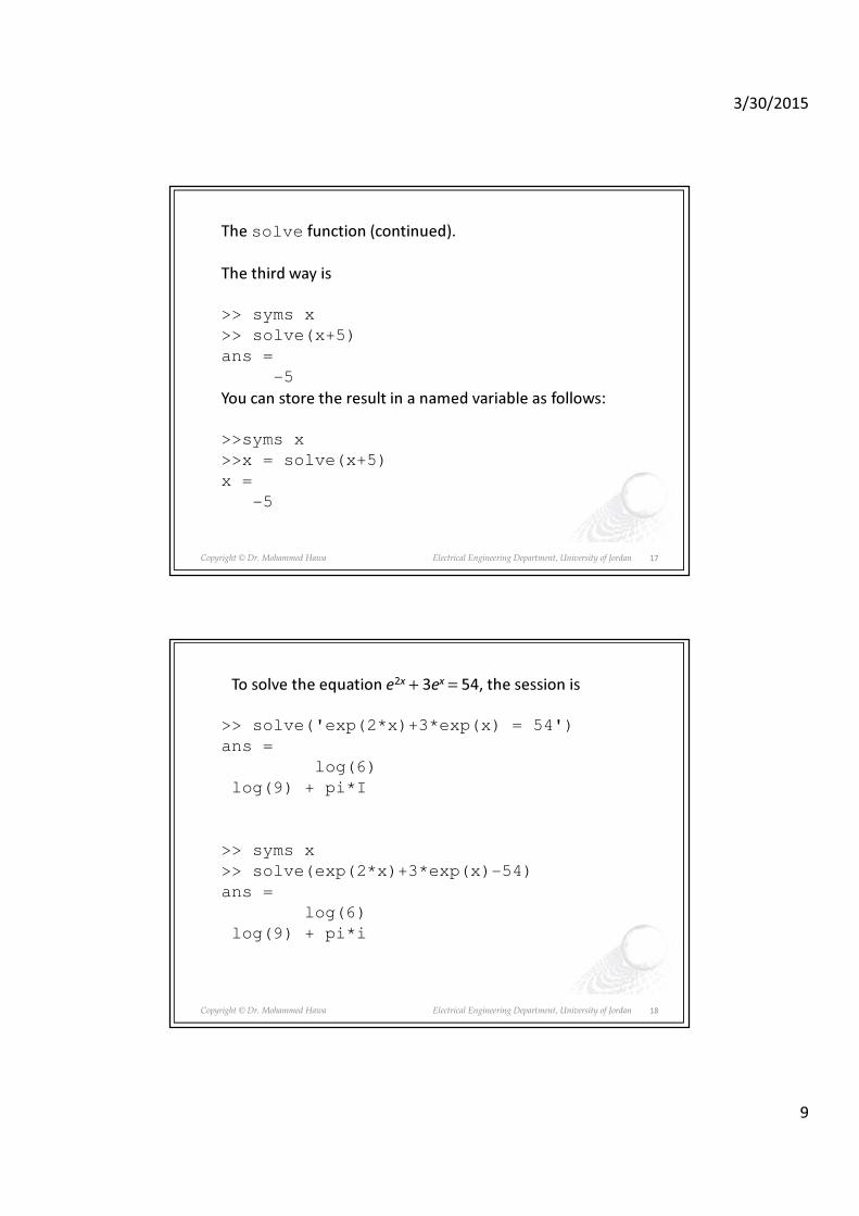
3/30/2015

9


The solve function (continued).

The third way is

>> syms x

>> solve(x+5)

ans =

-5

You can store the result in a named variable as follows:

>>syms x

>>x = solve(x+5)

x =

-5

17


To solve the equation e2x + 3ex = 54, the session is

>> solve('exp(2*x)+3*exp(x) = 54')

ans =

log(6)

log(9) + pi*I

>> syms x

>> solve(exp(2*x)+3*exp(x)-54)

ans =

log(6)

log(9) + pi*i

18

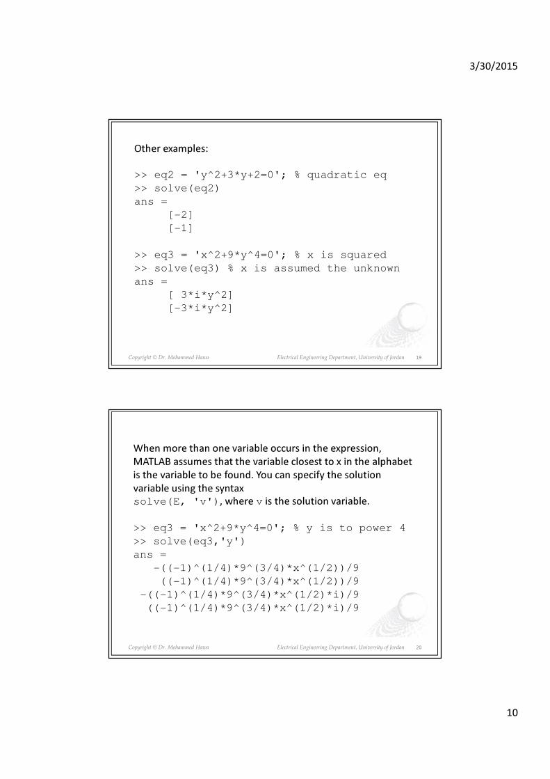
3/30/2015

10


Other examples:

>> eq2 = 'y^2+3*y+2=0'; % quadratic eq

>> solve(eq2)

ans =

[-2]

[-1]

>> eq3 = 'x^2+9*y^4=0'; % x is squared

>> solve(eq3) % x is assumed the unknown

ans =

[ 3*i*y^2]

[-3*i*y^2]

19


When more than one variable occurs in the expression,

MATLAB assumes that the variable closest to x in the alphabet

is the variable to be found. You can specify the solution

variable using the syntax

solve(E, 'v'), where v is the solution variable.

>> eq3 = 'x^2+9*y^4=0'; % y is to power 4

>> solve(eq3,'y')

ans =

-((-1)^(1/4)*9^(3/4)*x^(1/2))/9

((-1)^(1/4)*9^(3/4)*x^(1/2))/9

-((-1)^(1/4)*9^(3/4)*x^(1/2)*i)/9

((-1)^(1/4)*9^(3/4)*x^(1/2)*i)/9

20

3/30/2015

11


Application of the solve function: Find the two Intersection

points of the following two circles. Keep b unknown.

21


Solution

>> S = solve('(x-3)^2+(y-5)^2=4, (x-5)^2+(y-3)^2=b^2')

S =

x: [2x1 sym]

y: [2x1 sym]

>> S.x

ans =

(- b^4/16 + (3*b^2)/2 - 1)^(1/2)/2 - b^2/8 + 9/2

9/2 - b^2/8 - (- b^4/16 + (3*b^2)/2 - 1)^(1/2)/2

>> S.y

ans =

(- b^4/16 + (3*b^2)/2 - 1)^(1/2)/2 + b^2/8 + 7/2

b^2/8 - (- b^4/16 + (3*b^2)/2 - 1)^(1/2)/2 + 7/2

22

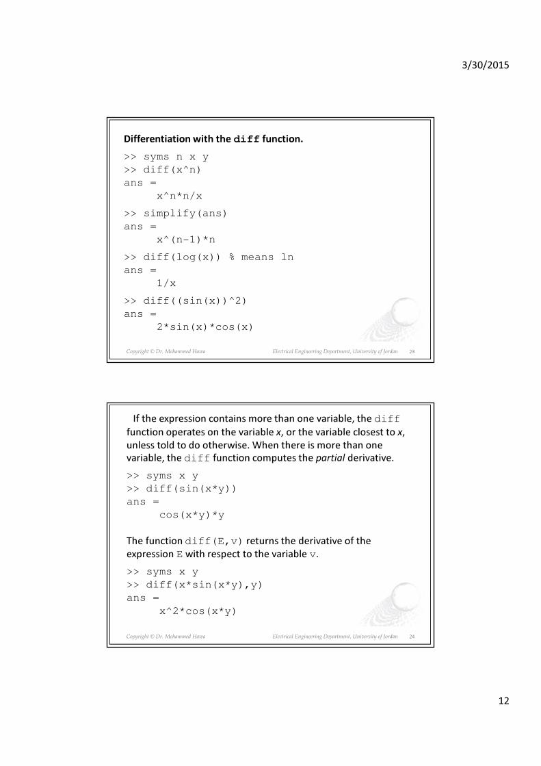
3/30/2015

12


Differentiation with the diff function.

>> syms n x y

>> diff(x^n)

ans =

x^n*n/x

>> simplify(ans)

ans =

x^(n-1)*n

>> diff(log(x)) % means ln

ans =

1/x

>> diff((sin(x))^2)

ans =

2*sin(x)*cos(x)

23


If the expression contains more than one variable, the diff

function operates on the variable x, or the variable closest to x,

unless told to do otherwise. When there is more than one

variable, the diff function computes the partial derivative.

>> syms x y

>> diff(sin(x*y))

ans =

cos(x*y)*y

The function diff(E,v) returns the derivative of the

expression E with respect to the variable v.

>> syms x y

>> diff(x*sin(x*y),y)

ans =

x^2*cos(x*y)

24

3/30/2015

13


The function diff(E,n) returns the nth derivative of the

expression E with respect to the default independent variable.

>> syms x

>> diff(x^3,2)

ans =

6*x

The function diff(E,v,n) returns the nth derivative of the

expression E with respect to the variable v.

>> syms x y

>> diff(x*sin(x*y),y,2)

ans =

-x^3*sin(x*y)

25


Integration with the int function.

>> syms x

>> int(2*x)

ans =

x^2

The function int(E) returns the integral of the expression

E with respect to the default independent variable.

26

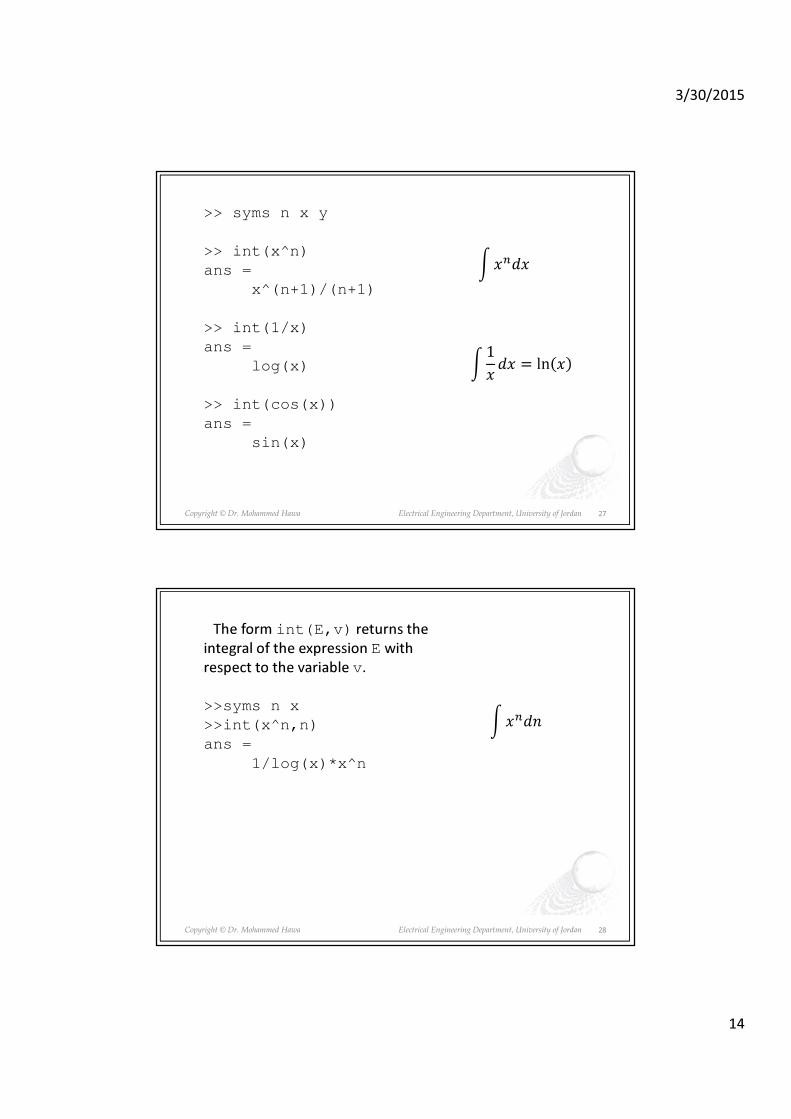
3/30/2015

14


>> syms n x y

>> int(x^n)

ans =

x^(n+1)/(n+1)

>> int(1/x)

ans =

log(x)

>> int(cos(x))

ans =

sin(x)

27

��

�1

� �� = ln �


The form int(E,v) returns the

integral of the expression E with

respect to the variable v.

>>syms n x

>>int(x^n,n)

ans =

1/log(x)*x^n

28

��

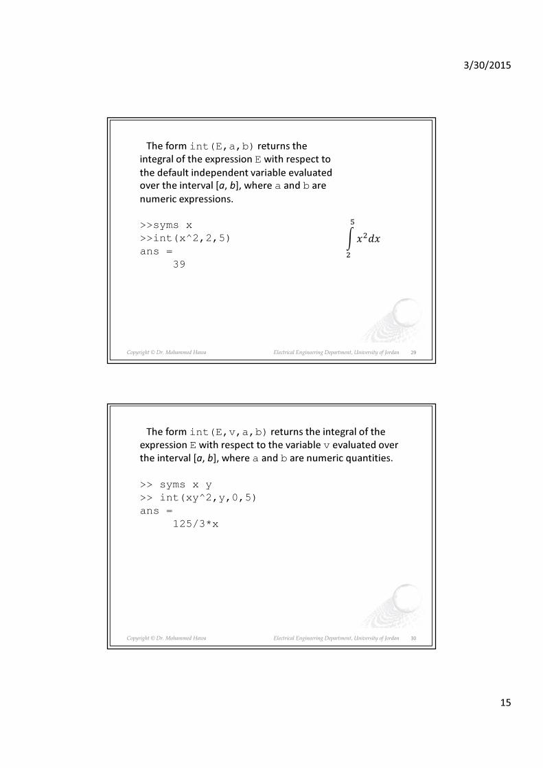
3/30/2015

15


The form int(E,a,b) returns the

integral of the expression E with respect to

the default independent variable evaluated

over the interval [a, b], where a and b are

numeric expressions.

>>syms x

>>int(x^2,2,5)

ans =

39

29

��

�


The form int(E,v,a,b) returns the integral of the

expression E with respect to the variable v evaluated over

the interval [a, b], where a and b are numeric quantities.

>> syms x y

>> int(xy^2,y,0,5)

ans =

125/3*x

30

3/30/2015

16


The form int(E,m,n) returns the integral of the

expression E with respect to the default independent

variable evaluated over the interval [m, n], where m and

n are symbolic expressions.

>> syms t x

>> int(x,1,t)

ans =

t^2/2 - 1/2

>> syms t x

>> int(sin(x),t,exp(t))

ans =

cos(t) - cos(exp(t))

31

��

�


The following session gives an example for which no

integral can be found. The indefinite integral exists,

but the definite integral does not exist if the limits of

integration include the singularity at x = 1.

>> syms x

>> int(1/(x-1))

ans =

log(x - 1)

>> syms x

>> int(1/(x-1),0,2)

ans =

NaN

32

3/30/2015

17


Taylor Series.

The taylor(f,n,a) function gives the first n-1 terms in

the Taylor series for the function defined in the expression f,

evaluated at the point x = a. If the parameter a is omitted the

function returns the series evaluated at x = 0.

>> syms x

>> f = exp(x);

>> taylor(f,3,2)

ans =

exp(2)+exp(2)*(x-2)+(exp(2)*(x-2)^2)/2

>> taylor(f,4)

ans =

x^3/6 + x^2/2 + x + 1

33

� � = � � + � − � �� +� − � �

2!�� +

� − � �

3!�(�) � +⋯


Series summation.

The symsum(E,a,b) function returns the sum of the

expression E as the default symbolic variable varies from a

to b.

>> syms k n

>> symsum(k,0,10)

ans =

55

>> symsum(k^2, 1, 4)

ans =

30

>> symsum(k,0,n-1)

ans =

(n*(n - 1))/2

34

��

��

��

��

3/30/2015

18


Finding limits.

The basic form limit(E) finds the limit as x → 0.

>> syms a x

>> limit(sin(a*x)/x)

ans =

a

35


The form limit(E,v,a) finds the limit as υ → a.

>>syms h x

>>limit((x-3)/(x^2-9),3)

ans =

1/6

>>limit((sin(x+h)-sin(x))/h,h,0)

ans =

cos(x)

36

3/30/2015

19


The forms limit(E,v,a,'right') and

limit(E,v,a,'left') specify the direction

of the limit.

>> syms x

>> limit(1/x,x,0,'left')

ans =

-inf

>> syms x

>> limit(1/x,x,0,'right')

ans =

inf

37


Solving differential equations with dsolve

The dsolve syntax for solving a single equation is

dsolve('eqn'). The function returns a

symbolic solution of the ODE specified by the

symbolic expression eqn.

>> dsolve('Dy+2*y=12')

ans =

6+C1*exp(-2*t)

There can be symbolic constants in the equation.

>> dsolve(’Dy=sin(a*t)’)

ans =

(-cos(a*t)+C1*a)/a

38

3/30/2015

20


Here is a second-order example:

>> dsolve('D2y=c^2*y')

ans =

C1*exp(-c*t) + C2*exp(c*t)

39


Sets of equations can be solved with dsolve. The appropriate

syntax is dsolve('eqn1','eqn2',...).

>>[x, y]=dsolve('Dx=3*x+4*y','Dy=-4*x+3*y')

x =

C1*exp(3*t)*cos(4*t)+C2*exp(3*t)*sin(4*t)

y = -

C1*exp(3*t)*sin(4*t)+C2*exp(3*t)*cos(4*t)

40

3/30/2015

21


Conditions on the solutions at specified values of the

independent variable can be handled as follows.

The form

dsolve('eqn', 'cond1', 'cond2',...)

returns a symbolic solution of the ODE specified by the

symbolic expression eqn, subject to the conditions

specified in the expressions cond1, cond2, and so on.

If y is the dependent variable, these conditions are

specified as follows: y(a) = b, Dy(a) = c,

D2y(a) = d, and so on.

41


Example:

>> dsolve('D2y=c^2*y','y(0)=1','Dy(0)=0')

ans =

1/2*exp(c*t)+1/2*exp(-c*t)

42

3/30/2015

22


Example:

>> [x,y]=dsolve('Dx=3*x+4*y','Dy=-4*x+3*y',

'x(0)=0','y(0)=1')

x =

sin(4*t)*exp(3*t)

y =

cos(4*t)*exp(3*t)

It is not necessary to specify only initial conditions. The

conditions can be specified at different values of t.

>> dsolve('D2y+9*y=0','y(0)=1','Dy(pi)=2')

ans =

cos(3*t) - (2*sin(3*t))/3

43


>> syms b t

>> laplace(t^3)

ans =

6/s^4

>> laplace(exp(-b*t))

ans =

1/(s+b)

>> laplace(sin(b*t))

ans =

b/(s^2+b^2)

>> fourier(exp(-t^2))

ans =

pi^(1/2)/exp(w^2/4)

Laplace and Fourier Transform

44

3/30/2015

23


>>syms b s

>>ilaplace(1/s^4)

ans =

1/6*t^3

>>ilaplace(1/(s+b))

ans =

exp(-b*t)

>>ilaplace(b/(s^2+b^2)

ans =

sin(b*t)

Laplace Inverse Transform

45


You can use the inv(A) and det(A) functions to invert and

find the determinant of a matrix symbolically.

>> syms k

>> A = [0 ,1;-k, -2];

>> inv(A)

ans =

[ -2/k, -1/k ]

[ 1, 0 ]

>> A*ans % verify inverse is correct

ans =

[ 1, 0 ]

[ 0, 1 ]

>> det(A)

ans =

k

46

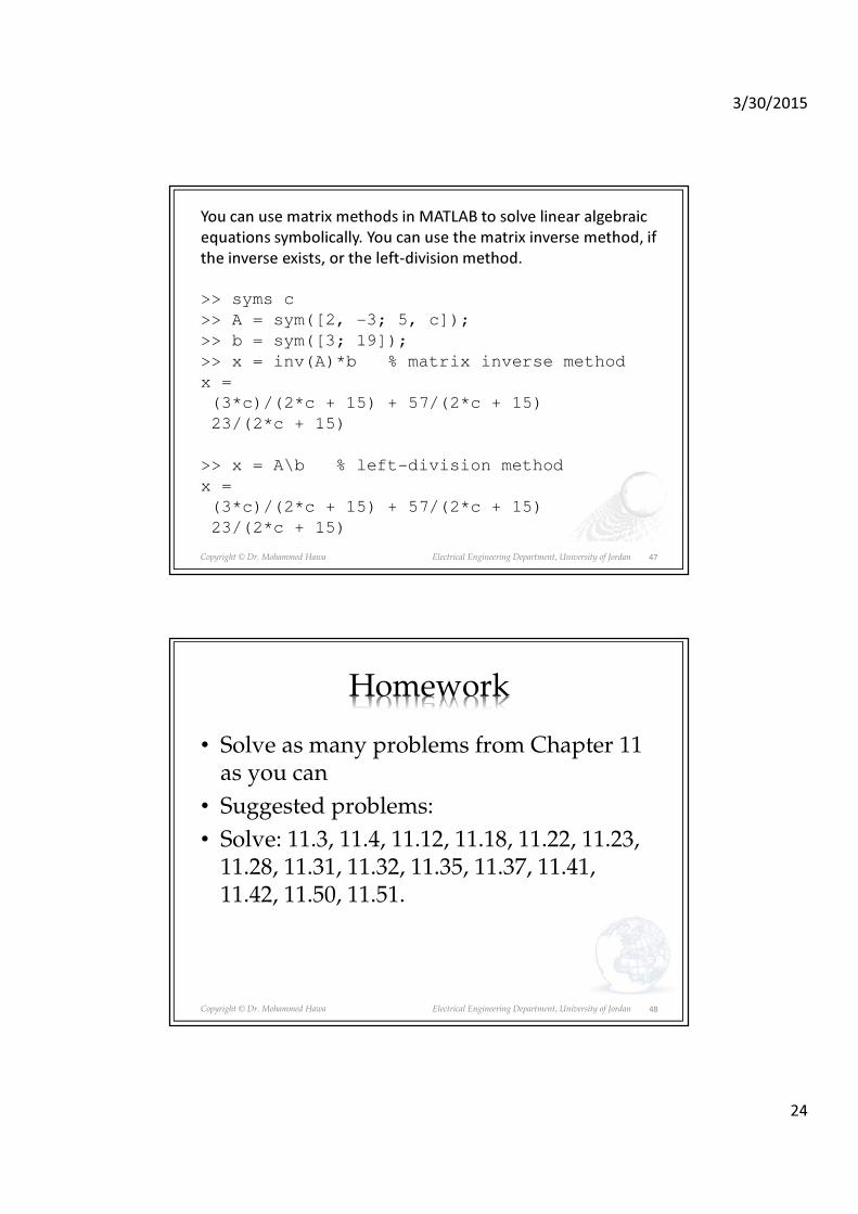
3/30/2015

24


You can use matrix methods in MATLAB to solve linear algebraic

equations symbolically. You can use the matrix inverse method, if

the inverse exists, or the left-division method.

>> syms c

>> A = sym([2, -3; 5, c]);

>> b = sym([3; 19]);

>> x = inv(A)*b % matrix inverse method

x =

(3*c)/(2*c + 15) + 57/(2*c + 15)

23/(2*c + 15)

>> x = A\b % left-division method

x =

(3*c)/(2*c + 15) + 57/(2*c + 15)

23/(2*c + 15)

47


Homework



• Solve: 11.3, 11.4, 11.12, 11.18, 11.22, 11.23, 11.28, 11.31, 11.32, 11.35, 11.37, 11.41, 11.42, 11.50, 11.51.

48

3/30/2015

1

Lecture 10: Simulink





What is Simulink?

• Simulink is a tool for modeling, simulating and analyzing dynamic systems.

• Its primary interface is a graphical block diagramming tool and a customizable set of block libraries.

• It supports linear and nonlinear systems, modeled in continuous time, discrete time, or a hybrid of both.

• It easily integrates with the rest of the MATLAB environment.

• Simulink is widely used in control theory and digital signal processing for simulation and model-based design.

2

3/30/2015

2


Starting Simulink

• To build a Simulink model, choose File | New | Model.

• To see the Simulink library of blocks click on the Simulink icon in MATLAB.

3


Library Browser & Model Window

4

3/30/2015

3


Drag & Drop

5


• Sources | Sine Wave• Continuous | Integrator• Signal Routing| Mux• Sinks | Scope• To connect blocks,

move the cursor to the output port represented by ">" sign. Once placed at a port, the cursor will turn into a cross "+" enabling you to make the connection between blocks.

• Run the simulation of the simple system shown by clicking on the play icon.

� � � � ��

�

� 1� �

6

3/30/2015

4


Scope Results

• Double click on the scope block to see the results of the simulation.

• To view/edit the parameters of a block, double click on the block to see the Block Parameters window.

• Try changing the initial condition of the Integrator from 0 to -1.

7


Blocks & Model File

• MATLAB uses the default values of the block parameters, except where you explicitly change them.

• You can always click on Help within the Block Parameters window to obtain more information.

• You can edit the label of a block by clicking on the text and making the changes.

• You can search for Blocks in the Simulink search window.

• You can save the Simulink model as .mdl file by selecting File | Save menu item in Simulink.

8

3/30/2015

5


Exercise: ModulationBlocks:

• Sources: Repeating Sequence

• Sources: Since Wave

• Math Operation: Product

• Math Operation: Gain

• Sinks: Scope

Edit the following properties:

• Repeating Sequence:– Time Values: [0 1 2 3 4 5 6]

– Output Values: [0 1 1 0 -1 -1 0]

• Sine Wave:• Frequency: 50 rad/s• Sample time: 0.01

• Gain: 2• Simulation Stop Time:

• 12 seconds

9


Results

10

3/30/2015

6


Exercise: Sending data to Workspace.

Notice the “Clock” and “To Workspace” blocks.

Set simulation time to 13 seconds.


Double-click on the To Workspace block. You can specify any

variable name you want as the output; the default is

simout. Change its name to y.

The output variable y will have as many rows as there are

simulation time steps, and as many columns as there are

inputs to the block.

The second column in our simulation will be time, because

of the way we have connected the Clock to the second

input port of the Mux.

Specify the Save format as Array. Use the default values for

the other parameters (these should be inf, 1, and -1 for

Maximum number of rows, Decimation, and Sample time,

respectively). Click on OK.

3/30/2015

7


Simulink can be configured to put the time variable tout

into the MATLAB workspace automatically when you are

using the To Workspace block.

This is done with the Data I/O tab under Configuration

Parameters on the Simulation menu.

The alternative is to use the Clock block to put tout into

the workspace.

The Clock block has one parameter, Decimation. Set this

parameter to 1, which means the Clock block will output

the time every time step; if set to 10 for example, the block

will output every 10 time steps, and so on.

In MATLAB, try: plot(y(:,2), y(:,1))


Result

0 2 4 6 8 10 12 140

2

4

6

8

10

12

14

16

18

20

14

3/30/2015

8


Simulation diagrams for x = dy/dt ==== 10 f (t )

Simulation diagram for dy/dt ==== f (t) −−−− 10y

= dy/dt

dy/dt


Exercise: Simulink model to solve the first-order ODE

dy/dt ==== −−−−10y ++++ 2sin(4t) � ≤ � ≤ �

Homework: Use Simulink to solve the second-order ODE

d2x/dt2 = 5cos(2t) -3 dx/dt - 4x � ≤ � ≤ �

3/30/2015

9


Result

17


Homework



• Solve: 10.1, 10.3, 10.4.

18

3/30/2015

1

Lecture 11: MATLAB Exercises





Exercise 1

• Write a MATLAB m-file function (called fact.m) which takes a single argument (an integer), computes the factorial and returns the answer.

• Hint: For better performance, do not use loops!

2

3/30/2015

2


Exercise 2

• Write a MATLAB m-file function (called grades.m) which accepts student grades as argument (hint: number array) and then determines the lowest, highest and average of such scores.

• E.g., grades([11 10 99 5 19 3 17])• Total: 7 scores

• Min value: 3

• Max value: 99

• Average value: 23.43

3


Exercise 3

• Write a MATLAB m-file function (dice.m) which simulates one or more dice with each die giving values from 1 to 6.

• The program takes a single argument which is the number of dice.

• The output should contain the values of the dice and also the probability for this combination of dice to occur. The probability is expressed as a decimal value between 0 and 1 with five decimal points.

• E.g., Rolling 3 dice: 4 1 6 (Probability: 0.00463)

4

3/30/2015

3


Exercise 4

>> rev

one

two

three

END

-> three

-> two

-> one

• Write a MATLAB script (called rev.m) which reads a number of strings from standard input and prints them in reverse order on the command window.

• The input sequence is terminated with the string END.

• Hint: Use a cell array!

5


Exercise 5

• Write a MATLAB script (called count.m) which reads a string from standard input and then counts the number of words in that string.

• E.g., “Everyone loves MATLAB” contains 3 words.

6

3/30/2015

4


Exercise 6

• The sum of the squares of the first ten integers is:

• 12 + 22 + ... + 102 = 385

• The square of the sum of the first ten integers is:

• (1 + 2 + ... + 10)2 = 552 = 3025

• Hence the difference between the sum of the squares of the first ten integer numbers and the square of the sum is 3025 − 385 = 2640.

• Find the difference between the sum of the squares of the first one hundred integer numbers and the square of the sum.

7


Exercise 7

• A prime number (or a prime) is an integer number greater than 1 that has no positive divisors other than 1 and itself.

• The first six prime numbers are: 2, 3, 5, 7, 11, and 13.

• We can see that the 6th prime is 13.

• Write a MATLAB script to print the first 50 prime numbers.

8

3/30/2015

5


Exercise 8

• A Pythagorean triplet is a set of three positive integer numbers, � � � � �, for which: ��

��

�

• For example, 32 + 42 = 9 + 16 = 25 = 52.

• There exists exactly one Pythagorean triplet for which � � � � � � 1000.

• Write a MATLAB script to find this triplet.

9


Exercise 9

• Starting in the top left corner of a 2×2 grid, and only being able to move to the right and down, there are exactly 6 routes to the bottom right corner (see the figure below).

• How many such routes are there through a 10×10 grid?

10

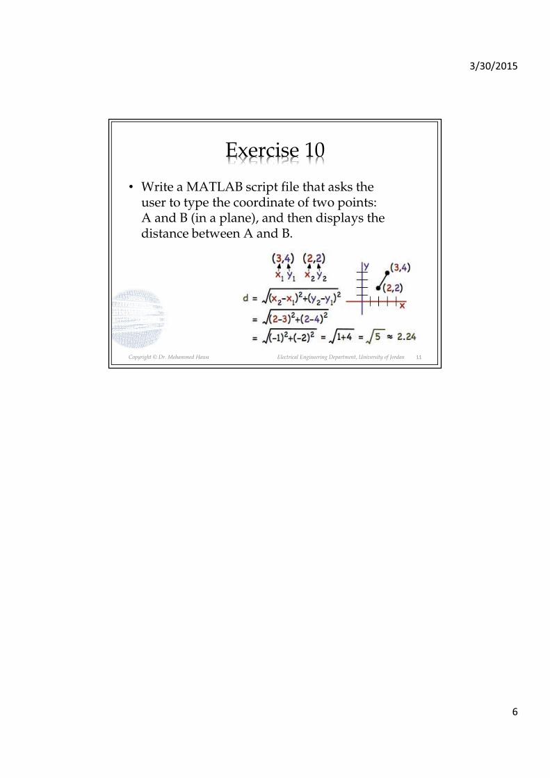
3/30/2015

6


Exercise 10

• Write a MATLAB script file that asks the user to type the coordinate of two points: A and B (in a plane), and then displays the distance between A and B.

11

of 2

The University of Jordan School of Engineering Department of Electrical Engineering 1st Semester – A.Y. 2014/2015

Course: Computer Applications – 0903201 (1 Cr. – Core Course)

Instructor: Dr. Mohammed Hawa Office: E306, Telephone: 5355000 ext 22857, Email: [email protected] Office Hours: will be posted soon

Course Website: http://fetweb.ju.edu.jo/staff/EE/mhawa/201/

Catalog Data: Computer packages for mathematical and symbolic manipulations (MATLAB, Mathematica). Windows environment. Graphics packages. INTERNET and its use in literature survey and information acquisition. Library search via computer. Engineering packages for computation. Data processing and statistical packages. Standard computer libraries.

Prerequisites by Course:

EE 1901102 – Computer Skills 2 (C++) (pre-requisite)

Prerequisites By Topic:

Students are assumed to have a background in the following topics:

• Basic computer and software skills.

• Basic programming language skills, such as C/C++.

• Basic mathematics, calculus and linear algebra.

• Basic scalar, array, vector and matrix operations.

• Solution of ordinary differential equations.

• Basic electric circuit analysis.

Textbook: Introduction to MATLAB for Engineers by William J. Palm III, McGraw-Hill, 3rd Edition, 2011.

References: • Essential MATLAB for Engineers and Scientists by Brian Hahn and Daniel Valentine, Academic Press, 5th Edition, 2013.

• MATLAB for Engineers by Holly Moore, Prentice Hall, 3rd Edition, 2011.

• Getting Started with MATLAB 7: A Quick Introduction for Scientists and Engineers by Rudra Pratap, Oxford University Press, 1st Edition, 2005.

• MATLAB Programming with Applications for Engineers by Stephen J. Chapman, CL-Engineering, 1st Edition, 2012.

• An Engineers Guide to MATLAB by Edward B. Magrab, et. al., Prentice Hall, 3rd Edition, 2010.

• Mastering MATLAB by Duane C. Hanselman and Bruce L. Littlefield, Prentice Hall, 1st Edition, 2011.

• Modeling and Simulation in SIMULINK for Engineers and Scientists by Mohammad Nuruzzaman, AuthorHouse; 1st Edition, 2005.

• Mastering Simulink by James B. Dabney and Thomas L. Harman, Prentice Hall, 1st Edition, 2003.

Schedule & Duration:

16 Weeks, 45 lectures (50 minutes each) plus exams.

Minimum Student Material:

Textbook, class handouts, scientific calculator, and an access to a personal computer.

Minimum College Facilities:

Classroom with whiteboard and projection display facilities, library, computational facilities with the MATLAB program.

Course Objectives:

The overall objective is to introduce the student to solving engineering problems using computers and scientific programming packages.

of 2

Course Learning Outcomes and Relation to ABET Student Outcomes: Upon successful completion of this course, a student should: 1. Use MATLAB to solve computational problems and generate publishable graphics [e, k] 2. Use complex arithmetic and complex functions to describe applied problems. Describe

complex numbers and functions in rectangular and exponential forms. Graph the magnitude and phase of complex functions

[a]

3. Use matrix forms to describe and solve linear systems of equations and systems of differential equations

[e]

4. Determine the system of linear equations required to find the coefficients that define an interpolating function that matches a set of data samples.

[a, e]

5. Solve first and second order linear differential equations with constant coefficients both analytically and numerically. Use the MATLAB routine ODE23 to solve differential equations numerically.

[a, k]

6. Define the Fourier series for a periodic signal. Define the Fourier transform of an aperiodic signal.

[a, k]

7. Compute the Fourier series and transform from their definition as integrals. [a, k] 8. Use the properties of linearity, time-shifting and time-scaling to compute the Fourier

series/transform of complex functions from the Fourier series/transforms of simple functions.

[a, k]

9. Use the Simulink simulation package to simulate some electric and electronic circuits [k]

Course Topics: Topic Description Hrs 1 Introduction to MATLAB and its use cases. Using the workspace to explore MATLAB features

regarding ease of use and versatility. Entering commands. Using MATLAB help. 2

2 General number formatting. Variables, Vectors and Matrices. Built-in MATLAB engineering functions. Matrix-related functions. Operator precedence. Matrix indexing: row and column versus linear versus logical indexing. Matrix versus element-by-elemtn operations.

3

3 Solving a system of linear equations. The concept of vectorization and its use in speeding computations.

2

4 Euclidean Vectors and their operations. Complex numbers. Polynomials. Cells arrays. Structures.

2

5 Script Files. Header comments. User Input/Output commands. The concept of functions in MATLAB and how to build user defined functions. Local vs. global variables. Subfunctions. Inline functions and function handles. Importing data: text, Excel, images, audio, etc.

3

6 Writing general-purpose programs in MATLAB. Flowchart versus pseudocode. Relational operators and conditional statements. Flow control structures and loops. Practical exercises.

4

7 Midterm Exam 1 8 Plotting. The different plot types available. Figure annotations. Three dimensional plots. 3 9 Using MATLAB buil-in functions to obtain numerical solutions for various calculus problems:

differentiation, integration, ordinary differential equations, etc. 2

10 MATLAB symbolic engine. Using symbolic notation to define and plot functions. Using symbolic capapilities for liner algebra, calcuals and other problems. Introduction to MuPAD.

2

11 Introduction to Simulink and its libraries. Simulating some engineering systems and finding solutions. Linking Simulink with the MATLAB workspace.

2

Ground Rules: Attendance is required and highly encouraged. To that end, attendance will be taken every lecture. All exams (including the final exam) should be considered cumulative. Exams are closed book. No scratch paper is allowed. You will be held responsible for all reading material assigned, even if it is not explicitly covered in lecture notes.

Assessments: Exams, Quizzes, Projects, and Assignments.

Grading policy: Assignments, projects, quizzes 20 % Midterm Exam 30 % Final Exam 50 %

Total 100%

Last Updated: January 2015

lecture 1: what is matlab? - power...

Documents