Lecture10:Capturingsemantics:WordEmbeddings

SanjeevArora EladHazan

COS402– MachineLearningand

ArtificialIntelligenceFall2016

(BorrowsfromslidesofD.Jurafsky StanfordU.)

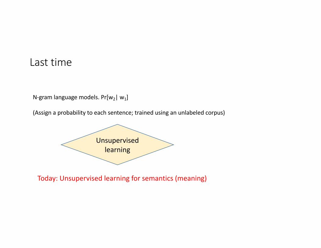
Lasttime

N-gramlanguagemodels.Pr[w2|w1]

(Assignaprobabilitytoeachsentence;trainedusinganunlabeledcorpus)

Unsupervisedlearning

Today:Unsupervisedlearningforsemantics(meaning)

Semantics

Studyofmeaningoflinguisticexpressions.

MasteringandfluentlyoperatingwithitseemsaprecursortoAI(Turingtest,etc.)

Buteverybitofpartialprogresscanimmediatelybeusedtoimprovetechnology:• Improvingwebsearch.• Siri,etc.• Machinetranslation• Informationretrieval,..

Let’stalkaboutmeaning

Whatdoesthesentence“Youlikegreencream”mean?”Comeupandseemesometime.”Howdidwordsarriveattheirmeanings?

Youranswersseemtoinvolveamixof

• Grammar/syntax• Howwordsmaptophysicalexperience• Physicalsensations“sweet”,“breathing”,“pain”etc.andmentalstates“happy,”“regretful”appear

tobeexperiencedroughlythesamewaybyeverybody,whichhelpanchorsome meanings)••• (atsomelevel,becomesphilosophy).

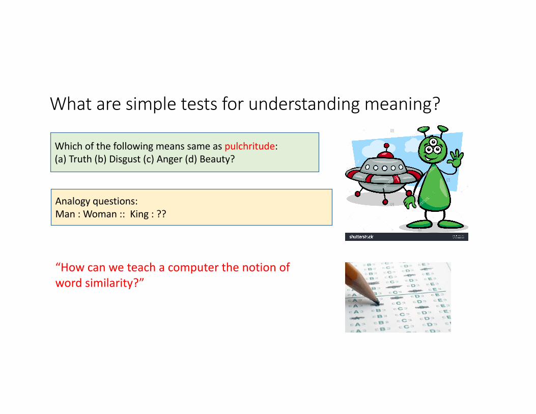
Whataresimpletestsforunderstandingmeaning?

Whichofthefollowingmeanssameaspulchritude:(a)Truth(b)Disgust(c)Anger(d)Beauty?

Analogyquestions:Man:Woman::King:??

“Howcanweteachacomputerthenotionofwordsimilarity?”

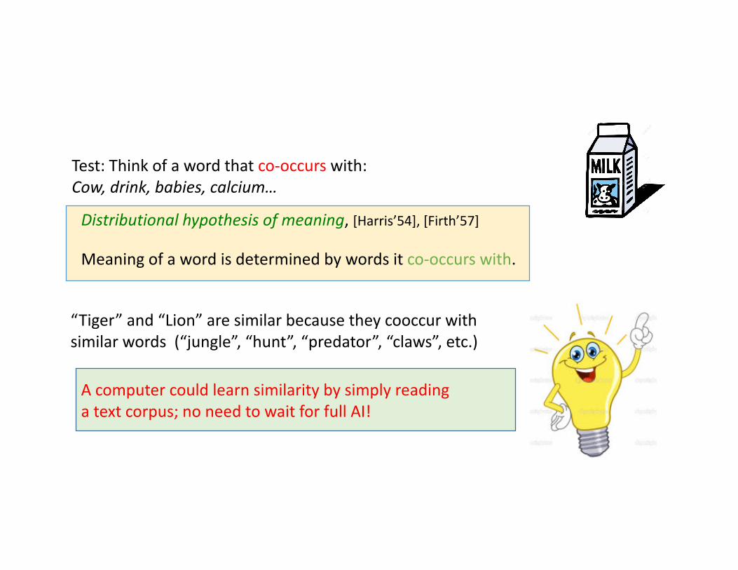
Test:Thinkofawordthatco-occurs with:Cow,drink,babies,calcium…

Distributionalhypothesisofmeaning,[Harris’54],[Firth’57]

Meaningofawordisdeterminedbywordsitco-occurswith.

“Tiger”and“Lion”aresimilarbecausetheycooccur withsimilarwords(“jungle”,“hunt”,“predator”,“claws”,etc.)

Acomputercouldlearnsimilaritybysimplyreadingatextcorpus;noneedtowaitforfullAI!

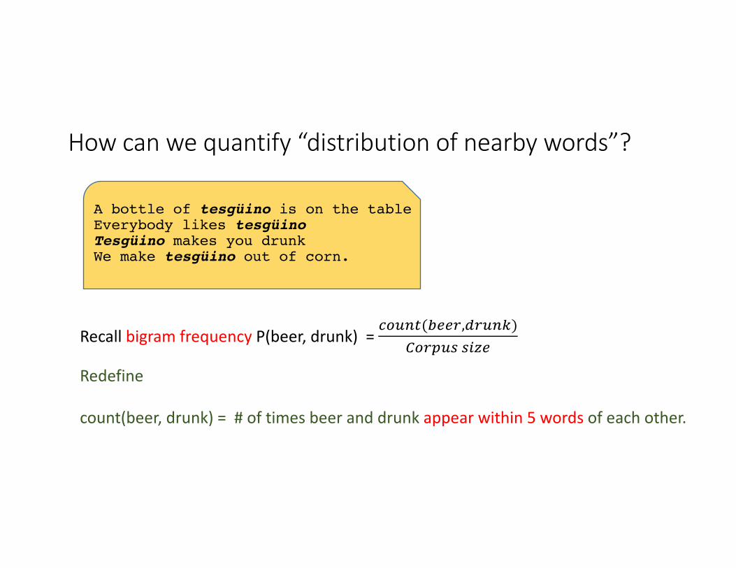
Howcanwequantify“distributionofnearbywords”?

A bottle of tesgüino is on the tableEverybody likes tesgüinoTesgüino makes you drunkWe make tesgüino out of corn.

Recallbigramfrequency P(beer,drunk)=!"#$%('((),+)#$,)

.")/#0023(

Redefine

count(beer,drunk)=#oftimesbeeranddrunkappearwithin5wordsofeachother.

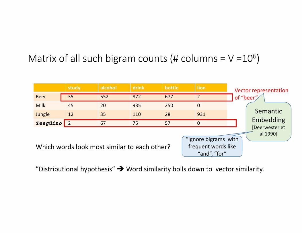
Matrixofallsuchbigramcounts(#columns=V=106)

study alcohol drink bottle lion

Beer 35 552 872 677 2

Milk 45 20 935 250 0

Jungle 12 35 110 28 931

Tesgüino 2 67 75 57 0

Whichwordslookmostsimilartoeachother?

Vectorrepresentationof“beer.”

”Distributionalhypothesis”èWordsimilarityboilsdowntovectorsimilarity.

SemanticEmbedding[Deerwester et

al1990]“Ignorebigrams withfrequentwordslike

“and”,“for”

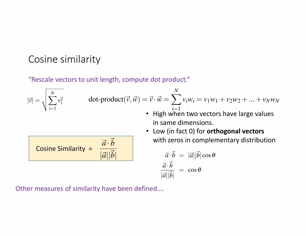
CosineSimilarity=

Cosinesimilarity

“Rescalevectorstounitlength,computedotproduct.”

19.2 • SPARSE VECTOR MODELS: POSITIVE POINTWISE MUTUAL INFORMATION 7

computer data pinch result sugarapricot 0 0 0.56 0 0.56

pineapple 0 0 0.56 0 0.56digital 0.62 0 0 0 0

information 0 0.58 0 0.37 0Figure 19.6 The Add-2 Laplace smoothed PPMI matrix from the add-2 smoothing countsin Fig. 17.5.

The cosine—like most measures for vector similarity used in NLP—is based onthe dot product operator from linear algebra, also called the inner product:dot product

inner product

dot-product(~v,~w) =~v ·~w =NX

i=1

viwi = v1w1 + v2w2 + ...+ vNwN (19.10)

Intuitively, the dot product acts as a similarity metric because it will tend to behigh just when the two vectors have large values in the same dimensions. Alterna-tively, vectors that have zeros in different dimensions—orthogonal vectors— will bevery dissimilar, with a dot product of 0.

This raw dot-product, however, has a problem as a similarity metric: it favorslong vectors. The vector length is defined asvector length

|~v| =

vuutNX

i=1

v2i (19.11)

The dot product is higher if a vector is longer, with higher values in each dimension.More frequent words have longer vectors, since they tend to co-occur with morewords and have higher co-occurrence values with each of them. Raw dot productthus will be higher for frequent words. But this is a problem; we’d like a similaritymetric that tells us how similar two words are irregardless of their frequency.

The simplest way to modify the dot product to normalize for the vector length isto divide the dot product by the lengths of each of the two vectors. This normalizeddot product turns out to be the same as the cosine of the angle between the twovectors, following from the definition of the dot product between two vectors ~a and~b:

~a ·~b = |~a||~b|cosq~a ·~b|~a||~b|

= cosq (19.12)

The cosine similarity metric between two vectors~v and ~w thus can be computedcosine

as:

cosine(~v,~w) =~v ·~w|~v||~w| =

NX

i=1

viwi

vuutNX

i=1

v2i

vuutNX

i=1

w2i

(19.13)

For some applications we pre-normalize each vector, by dividing it by its length,creating a unit vector of length 1. Thus we could compute a unit vector from ~a byunit vector

• Highwhentwovectorshavelargevaluesinsamedimensions.

• Low(infact0)fororthogonalvectorswith zerosincomplementarydistribution

19.2 • SPARSE VECTOR MODELS: POSITIVE POINTWISE MUTUAL INFORMATION 7

computer data pinch result sugarapricot 0 0 0.56 0 0.56

pineapple 0 0 0.56 0 0.56digital 0.62 0 0 0 0

information 0 0.58 0 0.37 0Figure 19.6 The Add-2 Laplace smoothed PPMI matrix from the add-2 smoothing countsin Fig. 17.5.

The cosine—like most measures for vector similarity used in NLP—is based onthe dot product operator from linear algebra, also called the inner product:dot product

inner product

dot-product(~v,~w) =~v ·~w =NX

i=1

viwi = v1w1 + v2w2 + ...+ vNwN (19.10)

Intuitively, the dot product acts as a similarity metric because it will tend to behigh just when the two vectors have large values in the same dimensions. Alterna-tively, vectors that have zeros in different dimensions—orthogonal vectors— will bevery dissimilar, with a dot product of 0.

This raw dot-product, however, has a problem as a similarity metric: it favorslong vectors. The vector length is defined asvector length

|~v| =

vuutNX

i=1

v2i (19.11)

The dot product is higher if a vector is longer, with higher values in each dimension.More frequent words have longer vectors, since they tend to co-occur with morewords and have higher co-occurrence values with each of them. Raw dot productthus will be higher for frequent words. But this is a problem; we’d like a similaritymetric that tells us how similar two words are irregardless of their frequency.

The simplest way to modify the dot product to normalize for the vector length isto divide the dot product by the lengths of each of the two vectors. This normalizeddot product turns out to be the same as the cosine of the angle between the twovectors, following from the definition of the dot product between two vectors ~a and~b:

~a ·~b = |~a||~b|cosq~a ·~b|~a||~b|

= cosq (19.12)

The cosine similarity metric between two vectors~v and ~w thus can be computedcosine

as:

cosine(~v,~w) =~v ·~w|~v||~w| =

NX

i=1

viwi

vuutNX

i=1

v2i

vuutNX

i=1

w2i

(19.13)

For some applications we pre-normalize each vector, by dividing it by its length,creating a unit vector of length 1. Thus we could compute a unit vector from ~a byunit vector

19.2 • SPARSE VECTOR MODELS: POSITIVE POINTWISE MUTUAL INFORMATION 7

computer data pinch result sugarapricot 0 0 0.56 0 0.56

pineapple 0 0 0.56 0 0.56digital 0.62 0 0 0 0

information 0 0.58 0 0.37 0Figure 19.6 The Add-2 Laplace smoothed PPMI matrix from the add-2 smoothing countsin Fig. 17.5.

The cosine—like most measures for vector similarity used in NLP—is based onthe dot product operator from linear algebra, also called the inner product:dot product

inner product

dot-product(~v,~w) =~v ·~w =NX

i=1

viwi = v1w1 + v2w2 + ...+ vNwN (19.10)

Intuitively, the dot product acts as a similarity metric because it will tend to behigh just when the two vectors have large values in the same dimensions. Alterna-tively, vectors that have zeros in different dimensions—orthogonal vectors— will bevery dissimilar, with a dot product of 0.

This raw dot-product, however, has a problem as a similarity metric: it favorslong vectors. The vector length is defined asvector length

|~v| =

vuutNX

i=1

v2i (19.11)

The dot product is higher if a vector is longer, with higher values in each dimension.More frequent words have longer vectors, since they tend to co-occur with morewords and have higher co-occurrence values with each of them. Raw dot productthus will be higher for frequent words. But this is a problem; we’d like a similaritymetric that tells us how similar two words are irregardless of their frequency.

The simplest way to modify the dot product to normalize for the vector length isto divide the dot product by the lengths of each of the two vectors. This normalizeddot product turns out to be the same as the cosine of the angle between the twovectors, following from the definition of the dot product between two vectors ~a and~b:

~a ·~b = |~a||~b|cosq~a ·~b|~a||~b|

= cosq (19.12)

The cosine similarity metric between two vectors~v and ~w thus can be computedcosine

as:

cosine(~v,~w) =~v ·~w|~v||~w| =

NX

i=1

viwi

vuutNX

i=1

v2i

vuutNX

i=1

w2i

(19.13)

For some applications we pre-normalize each vector, by dividing it by its length,creating a unit vector of length 1. Thus we could compute a unit vector from ~a byunit vector

19.2 • SPARSE VECTOR MODELS: POSITIVE POINTWISE MUTUAL INFORMATION 7

computer data pinch result sugarapricot 0 0 0.56 0 0.56

pineapple 0 0 0.56 0 0.56digital 0.62 0 0 0 0

information 0 0.58 0 0.37 0Figure 19.6 The Add-2 Laplace smoothed PPMI matrix from the add-2 smoothing countsin Fig. 17.5.

The cosine—like most measures for vector similarity used in NLP—is based onthe dot product operator from linear algebra, also called the inner product:dot product

inner product

dot-product(~v,~w) =~v ·~w =NX

i=1

viwi = v1w1 + v2w2 + ...+ vNwN (19.10)

Intuitively, the dot product acts as a similarity metric because it will tend to behigh just when the two vectors have large values in the same dimensions. Alterna-tively, vectors that have zeros in different dimensions—orthogonal vectors— will bevery dissimilar, with a dot product of 0.

This raw dot-product, however, has a problem as a similarity metric: it favorslong vectors. The vector length is defined asvector length

|~v| =

vuutNX

i=1

v2i (19.11)

The dot product is higher if a vector is longer, with higher values in each dimension.More frequent words have longer vectors, since they tend to co-occur with morewords and have higher co-occurrence values with each of them. Raw dot productthus will be higher for frequent words. But this is a problem; we’d like a similaritymetric that tells us how similar two words are irregardless of their frequency.

The simplest way to modify the dot product to normalize for the vector length isto divide the dot product by the lengths of each of the two vectors. This normalizeddot product turns out to be the same as the cosine of the angle between the twovectors, following from the definition of the dot product between two vectors ~a and~b:

~a ·~b = |~a||~b|cosq~a ·~b|~a||~b|

= cosq (19.12)

The cosine similarity metric between two vectors~v and ~w thus can be computedcosine

as:

cosine(~v,~w) =~v ·~w|~v||~w| =

NX

i=1

viwi

vuutNX

i=1

v2i

vuutNX

i=1

w2i

(19.13)

For some applications we pre-normalize each vector, by dividing it by its length,creating a unit vector of length 1. Thus we could compute a unit vector from ~a byunit vector

Othermeasuresofsimilarityhavebeendefined….

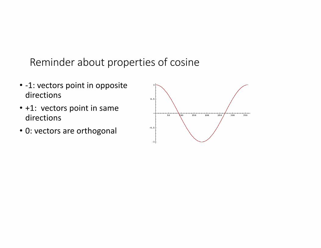
Reminderaboutpropertiesofcosine

• -1:vectorspointinoppositedirections• +1:vectorspointinsamedirections• 0:vectorsareorthogonal

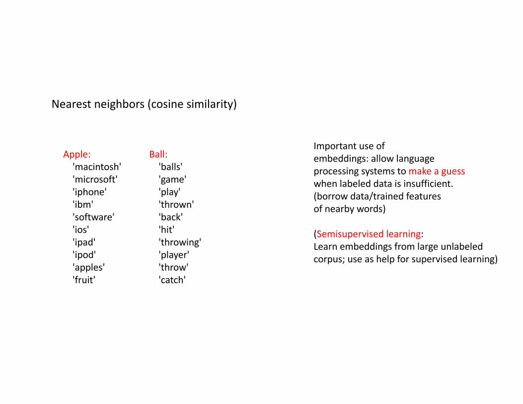
Nearestneighbors(cosinesimilarity)

Importantuseofembeddings:allowlanguageprocessing systemstomakeaguesswhenlabeleddataisinsufficient.(borrowdata/trainedfeaturesofnearbywords)

(Semisupervised learning:Learnembeddings fromlargeunlabeledcorpus;useashelpforsupervisedlearning)

Apple:'macintosh''microsoft''iphone''ibm''software''ios''ipad''ipod''apples''fruit'

Ball:'balls''game''play''thrown''back''hit''throwing''player''throw''catch'

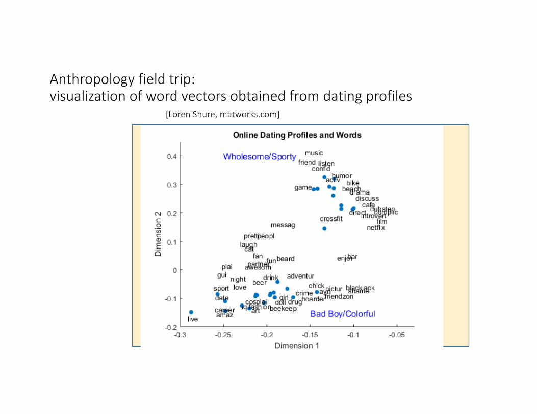
Anthropologyfieldtrip:visualizationofwordvectorsobtainedfromdatingprofiles

[LorenShure,matworks.com]

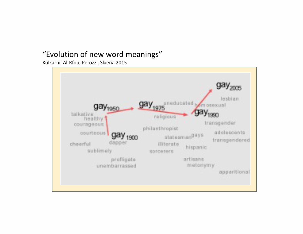
“Evolutionofnewwordmeanings”Kulkarni,Al-Rfou,Perozzi,Skiena 2015

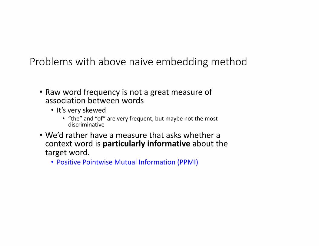
Problemswithabovenaiveembeddingmethod

• Rawwordfrequencyisnotagreatmeasureofassociationbetweenwords• It’sveryskewed

• “the”and“of”areveryfrequent,butmaybenotthemostdiscriminative

• We’dratherhaveameasurethataskswhetheracontextwordisparticularlyinformativeaboutthetargetword.• PositivePointwise MutualInformation(PPMI)

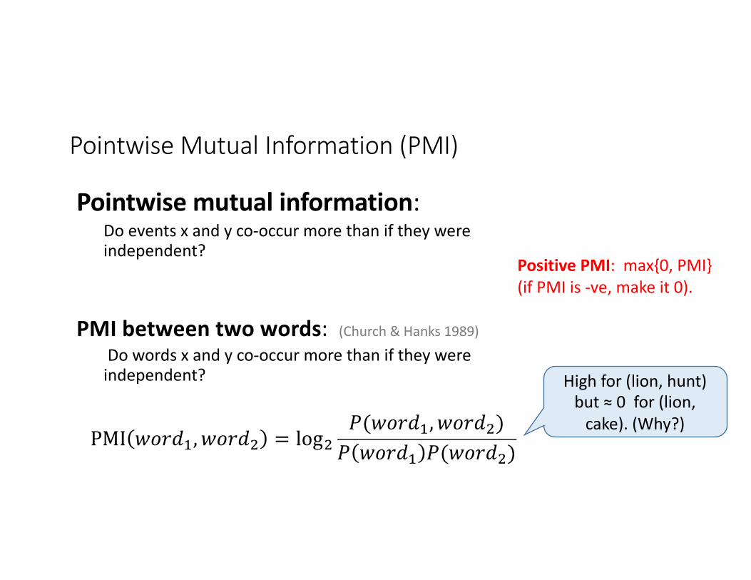
PointwiseMutualInformation(PMI)

Pointwisemutualinformation:Doeventsxandyco-occurmorethaniftheywereindependent?

PMIbetweentwowords:(Church&Hanks1989)Dowordsxandyco-occurmorethaniftheywereindependent?

PMI 𝑤𝑜𝑟𝑑;, 𝑤𝑜𝑟𝑑< = log<𝑃(𝑤𝑜𝑟𝑑;, 𝑤𝑜𝑟𝑑<)𝑃 𝑤𝑜𝑟𝑑; 𝑃(𝑤𝑜𝑟𝑑<)

PositivePMI:max{0,PMI}(ifPMIis-ve,makeit0).

Highfor(lion,hunt)but≈0for(lion,cake).(Why?)

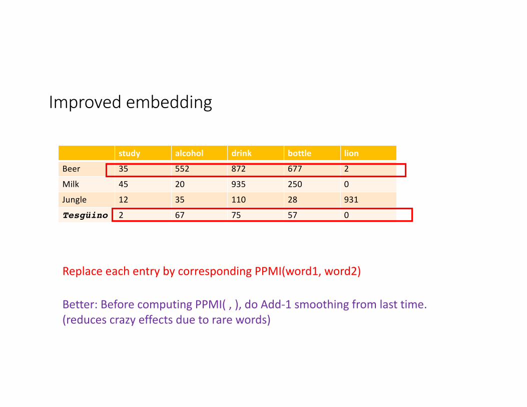
Improvedembedding

study alcohol drink bottle lion

Beer 35 552 872 677 2

Milk 45 20 935 250 0

Jungle 12 35 110 28 931

Tesgüino 2 67 75 57 0

ReplaceeachentrybycorrespondingPPMI(word1,word2)

Better:BeforecomputingPPMI(,),doAdd-1smoothingfromlasttime.(reducescrazyeffectsduetorarewords)

Implementationissues

• V=vocabularysize(say100,000)

• Thenwordembeddings definedaboveareV-dimensional.Veryclunkytocomputewith!(Willimprovesoon.)

• Wedefinedbigramsusing“windowsofsize5”

• Theshorterthewindows,themoresyntactic therepresentation± 1-3verysyntacticy

• Thelongerthewindows,themoresemantic therepresentation± 4-10moresemanticy

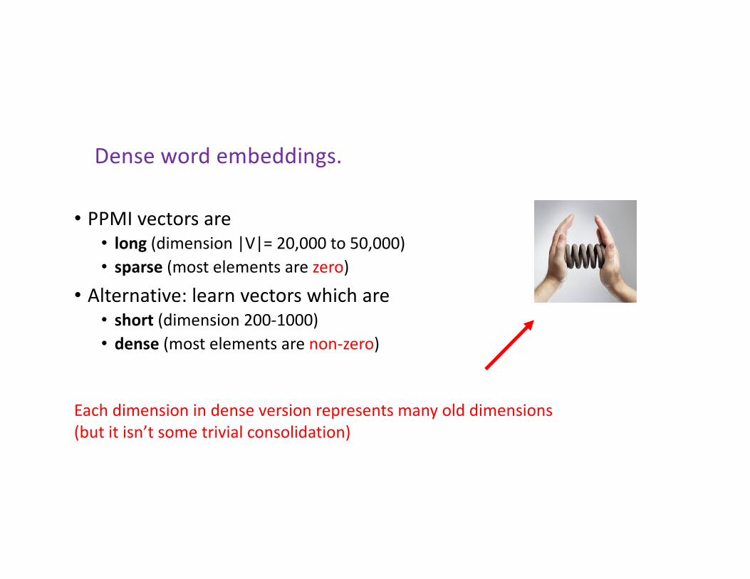
Densewordembeddings.

• PPMIvectorsare• long (dimension|V|=20,000to50,000)• sparse(mostelementsarezero)

• Alternative:learnvectorswhichare• short (dimension200-1000)• dense (mostelementsarenon-zero)

Eachdimensionindenseversionrepresentsmanyolddimensions(butitisn’tsometrivialconsolidation)

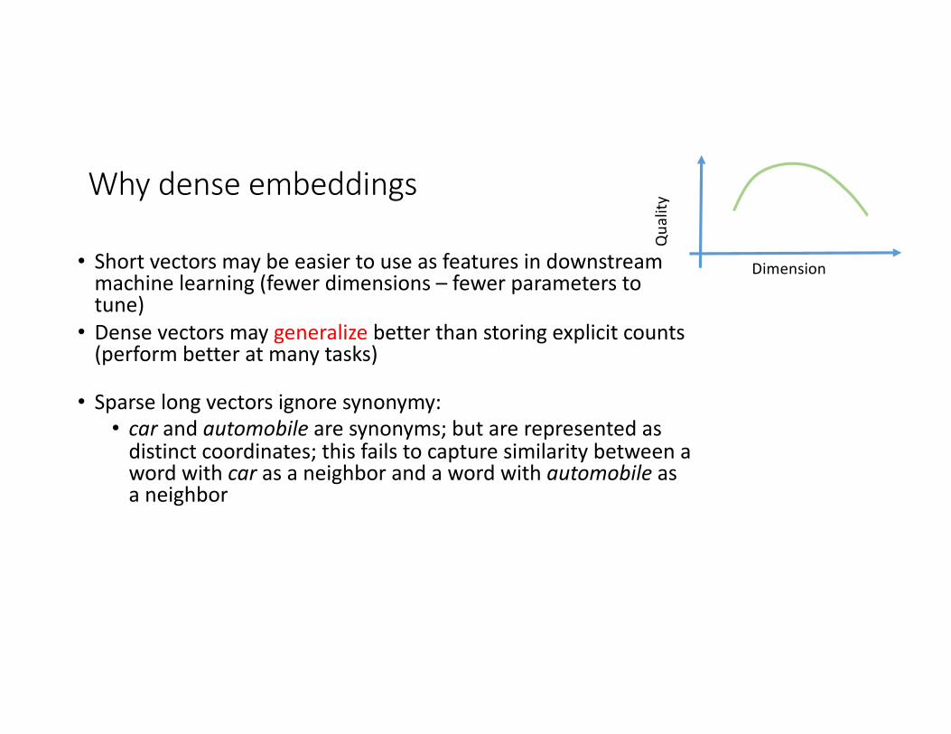
Whydenseembeddings

• Shortvectorsmaybeeasiertouseasfeaturesindownstreammachinelearning(fewerdimensions– fewerparameterstotune)• Densevectorsmaygeneralizebetterthanstoringexplicitcounts(performbetteratmanytasks)

• Sparselongvectorsignoresynonymy:• car andautomobile aresynonyms;butarerepresentedasdistinctcoordinates;thisfailstocapturesimilaritybetweenawordwithcar asaneighborandawordwithautomobile asaneighbor

Qua

lity

Dimension

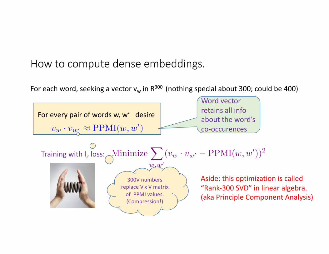
Howtocomputedenseembeddings.

Foreachword,seekingavectorvw inR300 (nothingspecialabout300;couldbe400)

Foreverypairofwordsw,w’desire

vw · vw0 ⇡ PPMI(w,w0)

Wordvectorretainsallinfoabouttheword’sco-occurences

Trainingwithl2 loss:

300VnumbersreplaceV xVmatrixofPPMIvalues.(Compression!)

Aside:thisoptimizationiscalled“Rank-300SVD”inlinearalgebra.(akaPrincipleComponentAnalysis)

MinimizeX

w,w0

(vw · vw0 � PPMI(w,w0))2

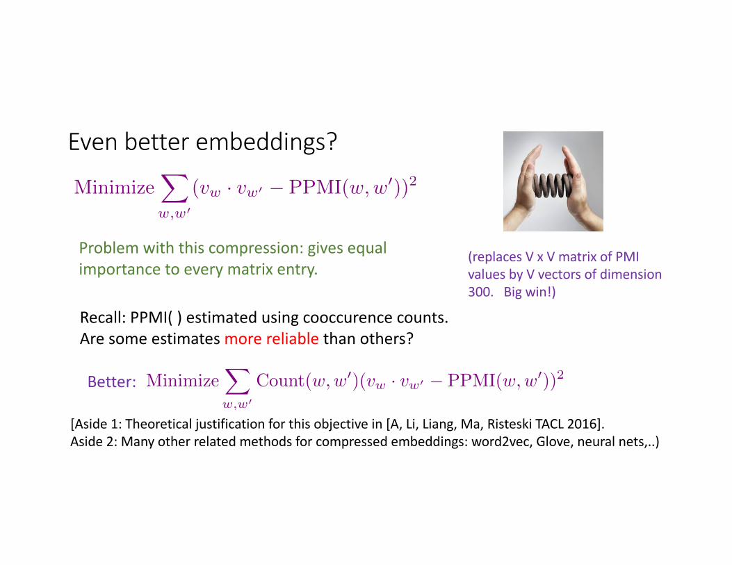
Evenbetterembeddings?

(replacesVxVmatrixofPMIvaluesbyVvectorsofdimension300. Bigwin!)

Problemwiththiscompression:givesequalimportancetoeverymatrixentry.

Recall:PPMI()estimatedusingcooccurence counts.Aresomeestimatesmorereliablethanothers?

[Aside1:Theoreticaljustificationforthisobjectivein[A,Li,Liang,Ma,Risteski TACL2016].Aside2:Manyotherrelatedmethodsforcompressedembeddings:word2vec,Glove,neuralnets,..)

Better:

MinimizeX

w,w0

(vw · vw0 � PPMI(w,w0))2

Minimize

X

w,w0

Count(w,w0)(vw · vw0 � PPMI(w,w0

))

2

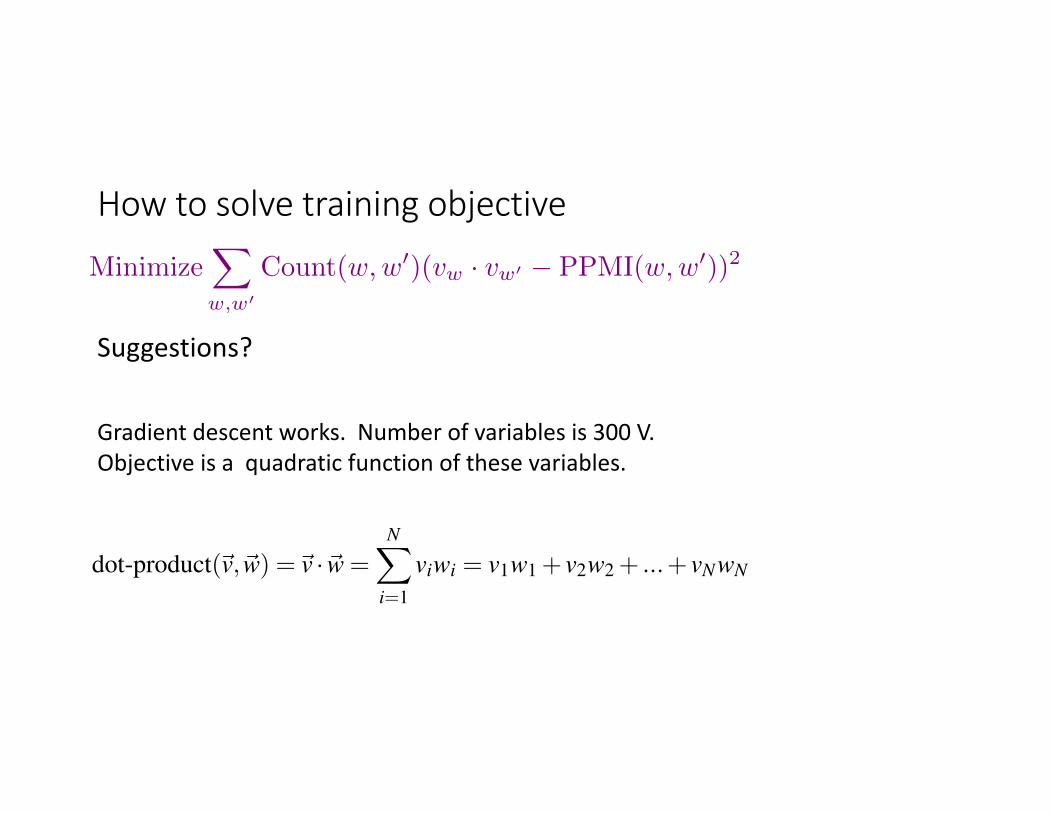
Howtosolvetrainingobjective

Suggestions?

Gradientdescentworks.Numberofvariablesis300V.Objectiveisaquadraticfunctionofthesevariables.

Minimize

X

w,w0

Count(w,w0)(vw · vw0 � PPMI(w,w0

))

2

19.2 • SPARSE VECTOR MODELS: POSITIVE POINTWISE MUTUAL INFORMATION 7

computer data pinch result sugarapricot 0 0 0.56 0 0.56

pineapple 0 0 0.56 0 0.56digital 0.62 0 0 0 0

information 0 0.58 0 0.37 0Figure 19.6 The Add-2 Laplace smoothed PPMI matrix from the add-2 smoothing countsin Fig. 17.5.

The cosine—like most measures for vector similarity used in NLP—is based onthe dot product operator from linear algebra, also called the inner product:dot product

inner product

dot-product(~v,~w) =~v ·~w =NX

i=1

viwi = v1w1 + v2w2 + ...+ vNwN (19.10)

Intuitively, the dot product acts as a similarity metric because it will tend to behigh just when the two vectors have large values in the same dimensions. Alterna-tively, vectors that have zeros in different dimensions—orthogonal vectors— will bevery dissimilar, with a dot product of 0.

This raw dot-product, however, has a problem as a similarity metric: it favorslong vectors. The vector length is defined asvector length

|~v| =

vuutNX

i=1

v2i (19.11)

The dot product is higher if a vector is longer, with higher values in each dimension.More frequent words have longer vectors, since they tend to co-occur with morewords and have higher co-occurrence values with each of them. Raw dot productthus will be higher for frequent words. But this is a problem; we’d like a similaritymetric that tells us how similar two words are irregardless of their frequency.

The simplest way to modify the dot product to normalize for the vector length isto divide the dot product by the lengths of each of the two vectors. This normalizeddot product turns out to be the same as the cosine of the angle between the twovectors, following from the definition of the dot product between two vectors ~a and~b:

~a ·~b = |~a||~b|cosq~a ·~b|~a||~b|

= cosq (19.12)

The cosine similarity metric between two vectors~v and ~w thus can be computedcosine

as:

cosine(~v,~w) =~v ·~w|~v||~w| =

NX

i=1

viwi

vuutNX

i=1

v2i

vuutNX

i=1

w2i

(19.13)

For some applications we pre-normalize each vector, by dividing it by its length,creating a unit vector of length 1. Thus we could compute a unit vector from ~a byunit vector

CoolpropertyofPMI-basedembeddings:Analogysolving(“word2vec”[Mikolov etal2013])

Man:Woman::King:??

vman

vwoman

vking

vqueen

Find w to minimize kvman

� vwoman

+ vking

� vw

k2

Warning:Suchpictures(plentifuloninternet)arev.misleading.Askmeaboutcorrectinterpretation

Someothercoolapplications(don’texpectyoutofullyunderstand;detailswon’tbeonexam)

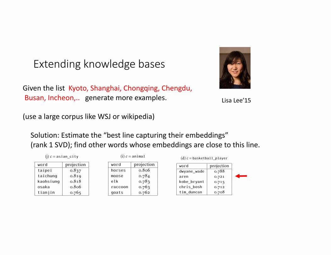
Extendingknowledgebases

Giventhelist Kyoto,Shanghai,Chongqing,Chengdu,Busan,Incheon,.. generatemoreexamples.

(usealargecorpuslikeWSJorwikipedia)

LisaLee’15

Solution:Estimatethe“bestlinecapturingtheirembeddings”(rank1SVD);findotherwordswhoseembeddings areclosetothisline.

On the Linear Structure of Word Embeddings Chapter 6. Extending a knowledge base | 26

(a) c = classical_composer

word projectionschumann 0.841beethoven 0.840stravinsky 0.796liszt 0.789schubert 0.788

(b) c = sport

word projectionbiking 0.881volleyball 0.870skiing 0.810softball 0.809soccer 0.801

(c) c = university

word projectioncambridge_university 0.897university_of_california 0.889new_york_university 0.868stanford_university 0.824yale_university 0.822

(d) c = basketball_player

word projectiondwyane_wade 0.788aren 0.721kobe_bryant 0.715chris_bosh 0.712tim_duncan 0.708

(e) c = religion

word projectionchristianity 0.899hinduism 0.880taoism 0.863buddhist 0.846judaism 0.830

(f) c = tourist_attraction

word projectionmetropolitan_museum_of_art 0.822museum_of_modern_art 0.813london 0.764national_gallery 0.764tate_gallery 0.756

(g) c = holiday

word projectiondiwali 0.821christmas 0.806passover 0.784new_year 0.783rosh_hashanah 0.749

(h) c = month

word projectionaugust 0.988april 0.987october 0.985february 0.983november 0.980

(i) c = animal

word projectionhorses 0.806moose 0.784elk 0.783raccoon 0.763goats 0.762

(j) c = asian_city

word projectiontaipei 0.837taichung 0.819kaohsiung 0.818osaka 0.806tianjin 0.765

Table 6.1: Given a set Sc

⇢ Dc

of words belonging to a category c, EXTEND_CATEGORY (Algorithm6.1) returns new words in D\S

c

which are also likely to belong to c. Here, we list the top 5 wordsreturned by EXTEND_CATEGORY(S

c

,k,�) for various categories c in Figure 4.1, using rank k = 10and threshold � = 0.6. The words w 2 D\S

c

are ordered in descending magnitude of the projectionkv

w

U

k

k onto the category subspace. The algorithm makes a few mistakes, e.g., it returns londonas a tourist_attraction, and aren as a basketball_player. But overall, the algorithm seems towork very well, and returns correct words that belong to the category.

On the Linear Structure of Word Embeddings Chapter 6. Extending a knowledge base | 26

(a) c = classical_composer

word projectionschumann 0.841beethoven 0.840stravinsky 0.796liszt 0.789schubert 0.788

(b) c = sport

word projectionbiking 0.881volleyball 0.870skiing 0.810softball 0.809soccer 0.801

(c) c = university

word projectioncambridge_university 0.897university_of_california 0.889new_york_university 0.868stanford_university 0.824yale_university 0.822

(d) c = basketball_player

word projectiondwyane_wade 0.788aren 0.721kobe_bryant 0.715chris_bosh 0.712tim_duncan 0.708

(e) c = religion

word projectionchristianity 0.899hinduism 0.880taoism 0.863buddhist 0.846judaism 0.830

(f) c = tourist_attraction

word projectionmetropolitan_museum_of_art 0.822museum_of_modern_art 0.813london 0.764national_gallery 0.764tate_gallery 0.756

(g) c = holiday

word projectiondiwali 0.821christmas 0.806passover 0.784new_year 0.783rosh_hashanah 0.749

(h) c = month

word projectionaugust 0.988april 0.987october 0.985february 0.983november 0.980

(i) c = animal

word projectionhorses 0.806moose 0.784elk 0.783raccoon 0.763goats 0.762

(j) c = asian_city

word projectiontaipei 0.837taichung 0.819kaohsiung 0.818osaka 0.806tianjin 0.765

Table 6.1: Given a set Sc

⇢ Dc

of words belonging to a category c, EXTEND_CATEGORY (Algorithm6.1) returns new words in D\S

c

which are also likely to belong to c. Here, we list the top 5 wordsreturned by EXTEND_CATEGORY(S

c

,k,�) for various categories c in Figure 4.1, using rank k = 10and threshold � = 0.6. The words w 2 D\S

c

are ordered in descending magnitude of the projectionkv

w

U

k

k onto the category subspace. The algorithm makes a few mistakes, e.g., it returns londonas a tourist_attraction, and aren as a basketball_player. But overall, the algorithm seems towork very well, and returns correct words that belong to the category.

On the Linear Structure of Word Embeddings Chapter 6. Extending a knowledge base | 26

(a) c = classical_composer

word projectionschumann 0.841beethoven 0.840stravinsky 0.796liszt 0.789schubert 0.788

(b) c = sport

word projectionbiking 0.881volleyball 0.870skiing 0.810softball 0.809soccer 0.801

(c) c = university

word projectioncambridge_university 0.897university_of_california 0.889new_york_university 0.868stanford_university 0.824yale_university 0.822

(d) c = basketball_player

word projectiondwyane_wade 0.788aren 0.721kobe_bryant 0.715chris_bosh 0.712tim_duncan 0.708

(e) c = religion

word projectionchristianity 0.899hinduism 0.880taoism 0.863buddhist 0.846judaism 0.830

(f) c = tourist_attraction

word projectionmetropolitan_museum_of_art 0.822museum_of_modern_art 0.813london 0.764national_gallery 0.764tate_gallery 0.756

(g) c = holiday

word projectiondiwali 0.821christmas 0.806passover 0.784new_year 0.783rosh_hashanah 0.749

(h) c = month

word projectionaugust 0.988april 0.987october 0.985february 0.983november 0.980

(i) c = animal

word projectionhorses 0.806moose 0.784elk 0.783raccoon 0.763goats 0.762

(j) c = asian_city

word projectiontaipei 0.837taichung 0.819kaohsiung 0.818osaka 0.806tianjin 0.765

Table 6.1: Given a set Sc

⇢ Dc

of words belonging to a category c, EXTEND_CATEGORY (Algorithm6.1) returns new words in D\S

c

which are also likely to belong to c. Here, we list the top 5 wordsreturned by EXTEND_CATEGORY(S

c

,k,�) for various categories c in Figure 4.1, using rank k = 10and threshold � = 0.6. The words w 2 D\S

c

are ordered in descending magnitude of the projectionkv

w

U

k

k onto the category subspace. The algorithm makes a few mistakes, e.g., it returns londonas a tourist_attraction, and aren as a basketball_player. But overall, the algorithm seems towork very well, and returns correct words that belong to the category.

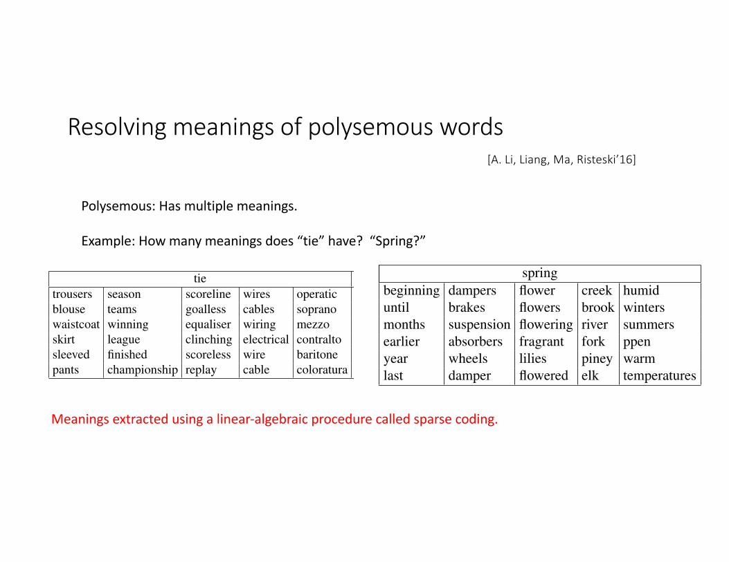
Resolvingmeaningsofpolysemous words[A.Li,Liang,Ma,Risteski’16]

Polysemous:Hasmultiplemeanings.

Example:Howmanymeaningsdoes“tie”have?“Spring?”

Atom 1978 825 231 616 1638 149 330drowning instagram stakes membrane slapping orchestra conferencessuicides twitter thoroughbred mitochondria pulling philharmonic meetingsoverdose facebook guineas cytosol plucking philharmonia seminarsmurder tumblr preakness cytoplasm squeezing conductor workshopspoisoning vimeo filly membranes twisting symphony exhibitionscommits linkedin fillies organelles bowing orchestras organizesstabbing reddit epsom endoplasmic slamming toscanini concertsstrangulation myspace racecourse proteins tossing concertgebouw lecturesgunshot tweets sired vesicles grabbing solti presentations

Table 1: Some discourse atoms and their nearest 9 words. By Eqn. (5), words most likely to appear in adiscourse are those nearest to it.

tie springtrousers season scoreline wires operatic beginning dampers flower creek humidblouse teams goalless cables soprano until brakes flowers brook winterswaistcoat winning equaliser wiring mezzo months suspension flowering river summersskirt league clinching electrical contralto earlier absorbers fragrant fork ppensleeved finished scoreless wire baritone year wheels lilies piney warmpants championship replay cable coloratura last damper flowered elk temperatures

Table 2: Five discourse atoms linked to the words tie and spring. Each atom is represented by its nearest 6words. The algorithm often makes a mistake in the last atom (or two), as happened here.

Similar overlapping clustering in a traditionalgraph-theoretic setup —clustering while simultane-ously cross-relating the senses of different words—seems more difficult but worth exploring.

4 Experiments with Atoms of DiscourseOur experiments use 300-dimensional embeddingscreated using objective (2) and a Wikipedia cor-pus of 3 billion tokens (Wikimedia, 2012), and thesparse coding is solved by standard k-SVD algo-rithm (Damnjanovic et al., 2010). Experimentationshowed that the best sparsity parameter k (i.e., themaximum number of allowed senses per word) is 5,and the number of atoms m is about 2000. This hy-perparameter choice is detailed below.

For the number of senses k, we tried plausiblealternatives (based upon suggestions of many col-leagues) that allow k to vary for different words,for example to let k be correlated with the wordfrequency. But a fixed choice of k = 5 seems toproduce as good results. To understand why, real-ize that WSI method retains no information aboutthe corpus except for the low dimensional word em-beddings. Since the sparse coding tends to expressa word using fairly different atoms, examining (6)shows that

!j α

2w,j is bounded by approximately

∥vw∥22. So if too many αw,j’s are allowed to benonzero, then some must necessarily have small co-efficients, which makes the corresponding compo-nents indistinguishable from noise. In other words,raising k often picks not only atoms correspondingto additional senses, but also many that don’t.

The best number of atoms m was found to bearound 2000. This was estimated by re-runningthe sparse coding algorithm multiple times with dif-ferent random initializations, whereupon substantialoverlap was found between the two bases: a largefraction of vectors in one basis were found to havea very close vector in the other. Thus combiningthe bases while merging duplicates yielded a basis ofabout the same size. Around 100 atoms are used bya large number of words or have no close by words.They appear semantically meaningless and are ex-cluded by checking for this condition.4

The content of each atom can be discerned bylooking at the nearby words in cosine similarity.Some examples are shown in Table 1. Each word isrepresented using at most five atoms, which usually

4We think semantically meaningless atoms —i.e., unex-plained inner products—exist because a simple language modelsuch as the random discourses model cannot explain all ob-served cooccurrences, and ends up needed smoothing terms.

Atom 1978 825 231 616 1638 149 330drowning instagram stakes membrane slapping orchestra conferencessuicides twitter thoroughbred mitochondria pulling philharmonic meetingsoverdose facebook guineas cytosol plucking philharmonia seminarsmurder tumblr preakness cytoplasm squeezing conductor workshopspoisoning vimeo filly membranes twisting symphony exhibitionscommits linkedin fillies organelles bowing orchestras organizesstabbing reddit epsom endoplasmic slamming toscanini concertsstrangulation myspace racecourse proteins tossing concertgebouw lecturesgunshot tweets sired vesicles grabbing solti presentations

Table 1: Some discourse atoms and their nearest 9 words. By Eqn. (5), words most likely to appear in adiscourse are those nearest to it.

tie springtrousers season scoreline wires operatic beginning dampers flower creek humidblouse teams goalless cables soprano until brakes flowers brook winterswaistcoat winning equaliser wiring mezzo months suspension flowering river summersskirt league clinching electrical contralto earlier absorbers fragrant fork ppensleeved finished scoreless wire baritone year wheels lilies piney warmpants championship replay cable coloratura last damper flowered elk temperatures

Table 2: Five discourse atoms linked to the words tie and spring. Each atom is represented by its nearest 6words. The algorithm often makes a mistake in the last atom (or two), as happened here.

Similar overlapping clustering in a traditionalgraph-theoretic setup —clustering while simultane-ously cross-relating the senses of different words—seems more difficult but worth exploring.

4 Experiments with Atoms of DiscourseOur experiments use 300-dimensional embeddingscreated using objective (2) and a Wikipedia cor-pus of 3 billion tokens (Wikimedia, 2012), and thesparse coding is solved by standard k-SVD algo-rithm (Damnjanovic et al., 2010). Experimentationshowed that the best sparsity parameter k (i.e., themaximum number of allowed senses per word) is 5,and the number of atoms m is about 2000. This hy-perparameter choice is detailed below.

For the number of senses k, we tried plausiblealternatives (based upon suggestions of many col-leagues) that allow k to vary for different words,for example to let k be correlated with the wordfrequency. But a fixed choice of k = 5 seems toproduce as good results. To understand why, real-ize that WSI method retains no information aboutthe corpus except for the low dimensional word em-beddings. Since the sparse coding tends to expressa word using fairly different atoms, examining (6)shows that

!j α

2w,j is bounded by approximately

∥vw∥22. So if too many αw,j’s are allowed to benonzero, then some must necessarily have small co-efficients, which makes the corresponding compo-nents indistinguishable from noise. In other words,raising k often picks not only atoms correspondingto additional senses, but also many that don’t.

The best number of atoms m was found to bearound 2000. This was estimated by re-runningthe sparse coding algorithm multiple times with dif-ferent random initializations, whereupon substantialoverlap was found between the two bases: a largefraction of vectors in one basis were found to havea very close vector in the other. Thus combiningthe bases while merging duplicates yielded a basis ofabout the same size. Around 100 atoms are used bya large number of words or have no close by words.They appear semantically meaningless and are ex-cluded by checking for this condition.4

The content of each atom can be discerned bylooking at the nearby words in cosine similarity.Some examples are shown in Table 1. Each word isrepresented using at most five atoms, which usually

4We think semantically meaningless atoms —i.e., unex-plained inner products—exist because a simple language modelsuch as the random discourses model cannot explain all ob-served cooccurrences, and ends up needed smoothing terms.

Meaningsextractedusingalinear-algebraicprocedurecalledsparsecoding.

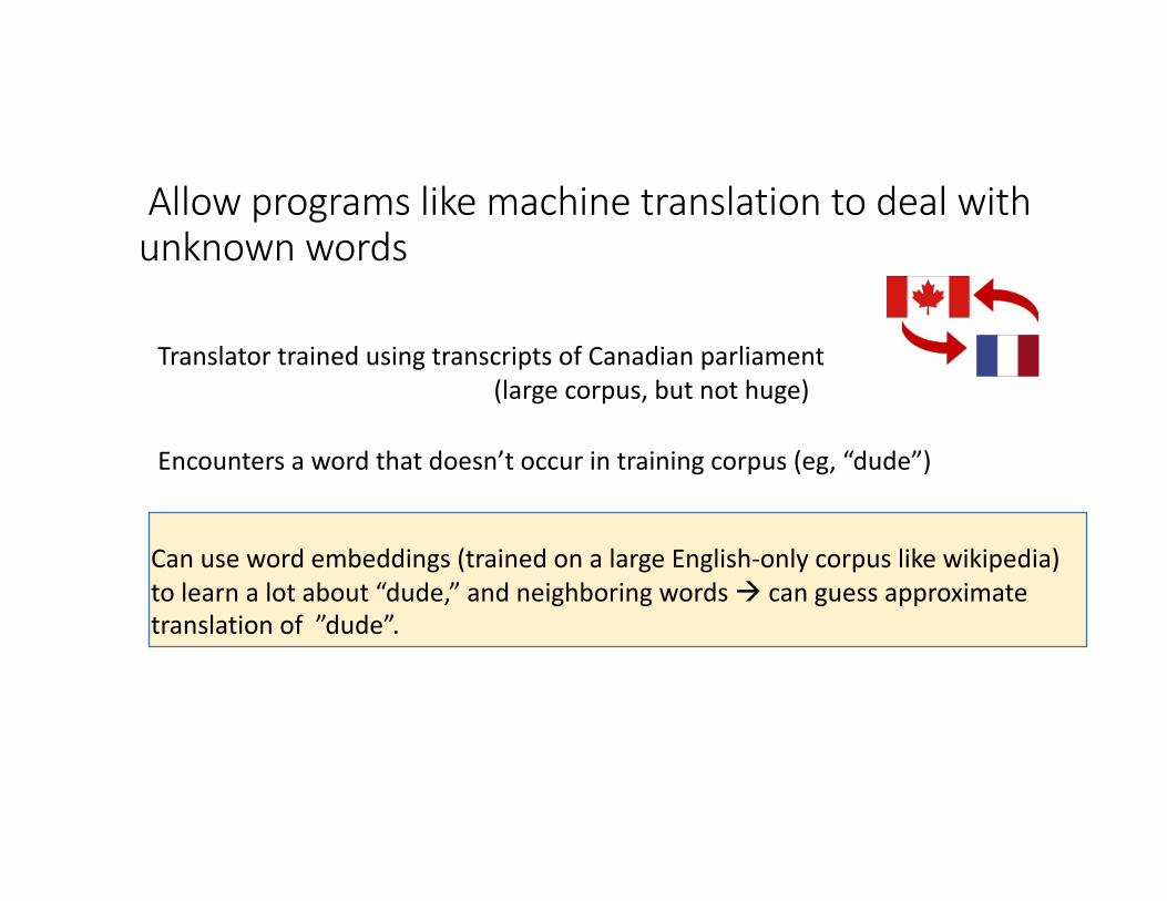
Allowprogramslikemachinetranslationtodealwithunknownwords

TranslatortrainedusingtranscriptsofCanadianparliament(largecorpus,butnothuge)

Encountersawordthatdoesn’toccurintrainingcorpus(eg,“dude”)

Canusewordembeddings (trainedonalargeEnglish-onlycorpuslikewikipedia)tolearnalotabout“dude,”andneighboringwordsà canguessapproximatetranslationof”dude”.

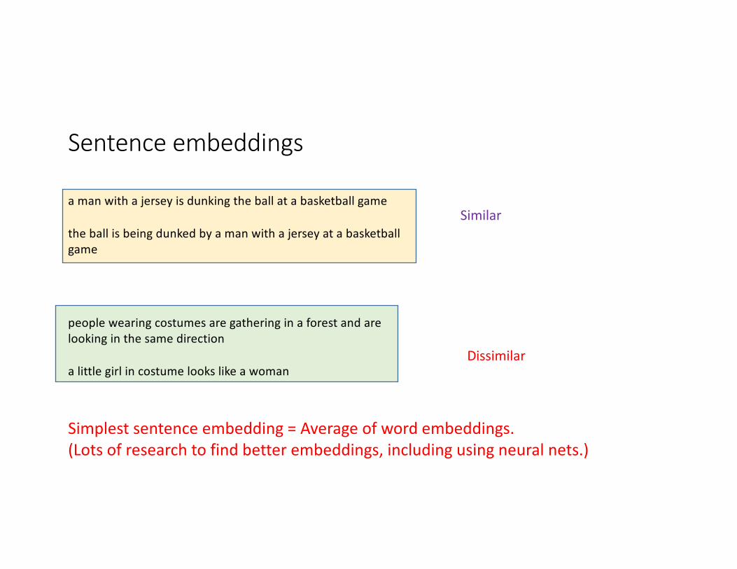
Sentenceembeddings

amanwithajerseyisdunkingtheballatabasketballgame

theballisbeingdunkedbyamanwithajerseyatabasketballgame

Similar

peoplewearingcostumesaregatheringinaforestandarelookinginthesamedirection

alittlegirlincostumelookslikeawomanDissimilar

Simplestsentenceembedding=Averageofwordembeddings.(Lotsofresearchtofindbetterembeddings,includingusingneuralnets.)

Nextlecture:Collaborativefiltering

(eg movieormusicrecommendersystems)

Homeworkisouttoday;duenextTues

Midterm:AweekfromThurs.