lecture 10: pivot - ucla statistics | websitecocteau/stat105/lectures/lecture10.pdflecture 10: pivot...

Lecture 10: Pivot

• Last time

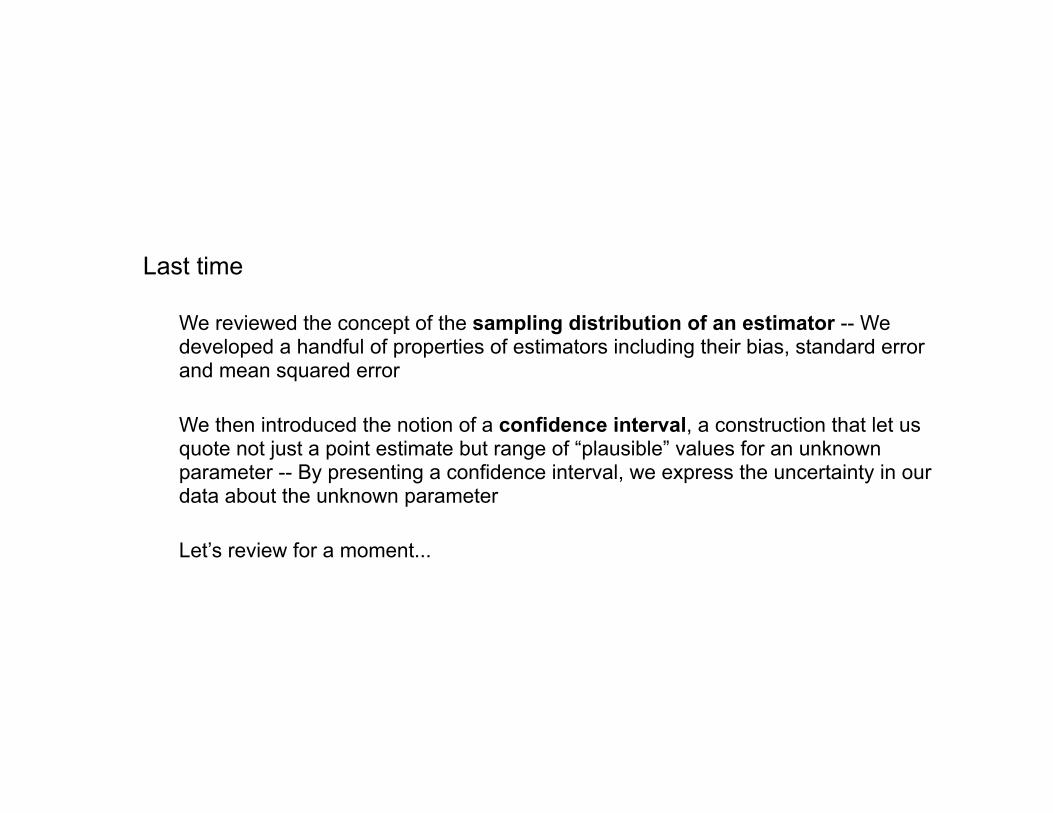
• We reviewed the concept of the sampling distribution of an estimator -- We developed a handful of properties of estimators including their bias, standard error and mean squared error

• We then introduced the notion of a confidence interval, a construction that let us quote not just a point estimate but range of “plausible” values for an unknown parameter -- By presenting a confidence interval, we express the uncertainty in our data about the unknown parameter

• Let’s review for a moment...

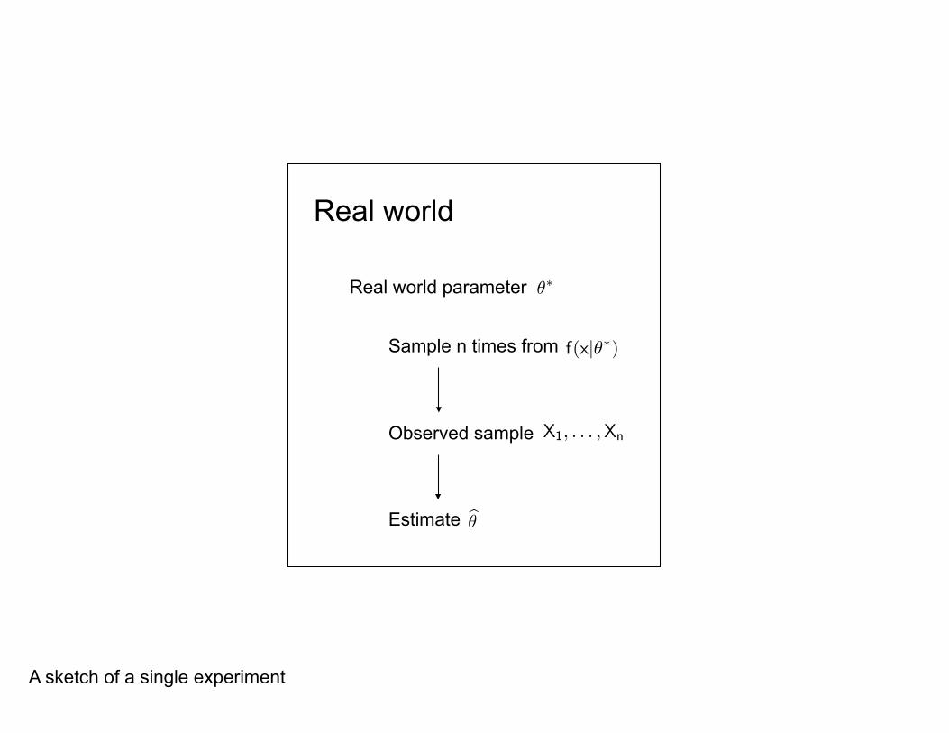
Real world

Real world parameter

Sample n times from

Observed sample

Estimate

✓⇤

f(x|✓⇤)

X1, . . . ,Xn

b✓

A sketch of a single experiment

Real world


Sample n times from

Observed sample

Estimate

✓⇤

f(x|✓⇤)

X1, . . . ,Xn

b✓ b✓

A sketch of a single experiment and an estimate

Real world


Sample n times from

Observed sample

Estimate

✓⇤

f(x|✓⇤)

X1, . . . ,Xn

b✓

Real world


Sample n times from

Observed sample

Estimate

✓⇤

f(x|✓⇤)

X1, . . . ,Xn

b✓

Repeating the experiment produces new data and a new estimate...

b✓1

b✓2

Real world


Sample n times from

Observed sample

Estimate

✓⇤

f(x|✓⇤)

X1, . . . ,Xn

b✓

Real world


Sample n times from

Observed sample

Estimate

✓⇤

f(x|✓⇤)

X1, . . . ,Xn

b✓

Real world


Sample n times from

Observed sample

Estimate

✓⇤

f(x|✓⇤)

X1, . . . ,Xn

b✓

Real world


Sample n times from

Observed sample

Estimate

✓⇤

f(x|✓⇤)

X1, . . . ,Xn

b✓

Real world


Sample n times from

Observed sample

Estimate

✓⇤

f(x|✓⇤)

X1, . . . ,Xn

b✓

Repeating the experiment produces new data and a new estimate...

b✓1

b✓2

b✓3

b✓4

b✓5 ...

• The sampling distribution

• The distribution of the estimates computed from repeating our experiment multiple times is known as the sampling distribution -- As a theoretical quantity, it tells us about how well our estimate is performing

• Last time, we examined the mean of this distribution for bias in an estimate, used the spread to quantify the precision of an estimate, and introduced a construction that could be used to suggest “plausible” values for the unknown parameter given our data

• A simple case

• We ended the last lecture with a simple example -- Suppose we have n independent observations from the normal distribution with mean and variance

• You know from your probability class that the sample mean has a normal distribution (exactly) with mean and standard deviation

• Finally, again appealing to your probability course, we know that the quantity

• has a standard normal distribution -- Let’s put this result to work!

X1, . . . ,Xn µ �2

�/pnµ

X� µ

�/pn

X =Pn

i=1 Xi/n

• A simple case

• Because approximately 95% of the mass of the standard normal distribution is between +/-2

• we can move the downstairs in the fraction out to give

• or with one more move

P

✓�2 X� µ

�/pn 2

◆⇡ 0.95

P��2�/

pn X� µ 2�/

pn�⇡ 0.95

P�X� 2�/

pn µ X+ 2�/

pn�⇡ 0.95

• A simple case

• Suppose we are given n samples from the normal distribution with unknown mean and known standard deviation

• The MLE for is just the sample mean

• From our results on the previous slides, we know the sampling distribution of our MLE exactly -- It is normal with mean and standard deviation

• Using our terminology from the last couple lectures, we say that is unbiased and that its standard error is

µX1, . . . ,Xn

µ

�

X =nX

i=1

Xi/n

µ µ �/pn

�/pn

X

• A simple case

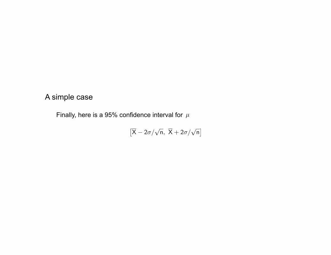
• Finally, here is a 95% confidence interval for

•

⇥X� 2�/

pn, X+ 2�/

pn⇤

µ

●●

●●

●●

●●

●●

●●

●●

●●

●●

●●

●●

●●

●●

●●

●●

●●

●●

●●

●●

●●

●●

●●

●●●

●●

●●●

●●

●●

●●●

●●

●●●

●●

●●

●●

●●

●●

●●

●●●

●●

●●

●●

●●

●●

●●

●●●

●●

●●

●●

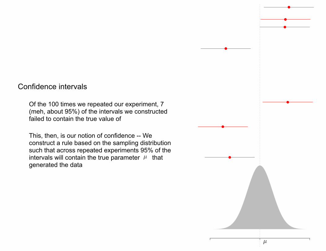
• Confidence intervals

• To make this concrete, at the top each black dot represents an experimental result -- We generated a sample and formed the MLE

• There are 100 black dots, representing 100 different sets of experimental outcomes -- The black dots are observations then from the sampling distribution and we can think of them as

X

X1, . . . ,X100

µ


• For each estimate, or, rather, each time we perform our experiment, we can then form a 95% confidence interval

• Given their construction, 95% of these intervals should cover the true parameter -- What do you think?

●●

●●

●●

●●

●●

●●

●●

●●

●●

●●

●●

●●

●●

●●

●●

●●

●●

●●

●●

●●

●●

●●

●●●

●●

●●●

●●

●●

●●●

●●

●●●

●●

●●

●●

●●

●●

●●

●●●

●●

●●

●●

●●

●●

●●

●●●

●●

●●

●●

X± 2�/pn

µ

µ

●

●

●

●

●

●

●


• Of the 100 times we repeated our experiment, 7 (meh, about 95%) of the intervals we constructed failed to contain the true value of

• This, then, is our notion of confidence -- We construct a rule based on the sampling distribution such that across repeated experiments 95% of the intervals will contain the true parameter that generated the data

µ

µ

• A snag

• This simple example isn’t quite practical because we rarely have situations in which we know -- And while our interest may be in the mean, we still need to estimate to form a confidence interval

• As we’ve seen, we can estimate using the MLE (or method of moments estimate)

• or the unbiased alternative

• What impact does “plugging in” an estimate for have on our confidence interval?

�

vuut1

n

nX

i=1

(Xi � X)2

vuut 1

n� 1

nX

i=1

(Xi � X)2

�

�

Before I had succeeded in solving my problem analytically, I had endeavoured to do so empirically. The material used was a correlation table containing the height and left middle finger measurements of 3000 criminals, from a paper by W. R. Macdonell. The measurements were written out on 3000 pieces of cardboard, which were then very thoroughly shuffled and drawn at random. As each card was drawn its numbers were written down in a book which thus contains the measurements of 3000 criminals in a random order. Finally each consecutive set of 4 was taken as a sample - 750 in all - and the mean, standard deviation and correlation of each sample determined. The difference between the mean of each sample and the mean of the population was then divided by the standard deviation of the sample...

has value less than 0.95

is our sample size

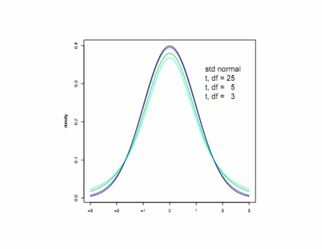
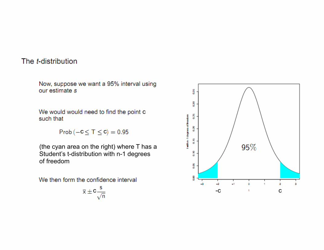
(the cyan area on the right) where T has a Student’s t-distribution with n-1 degrees of freedom

c c

c

c -c c

• Pivots

• Notice that when our data come from a normal distribution, then the quantity

• has the same distribution no matter what values of and were used to generate the data

• A quantity of this kind is known as a “pivot” -- As we have seen, pivots can be inverted to compute confidence intervals (this was the key ingredient in our chain of probability statements that pivoted our parameter of interest into the middle of our interval expression)

X� µ

s/pn

X1, . . . ,Xn

µ �

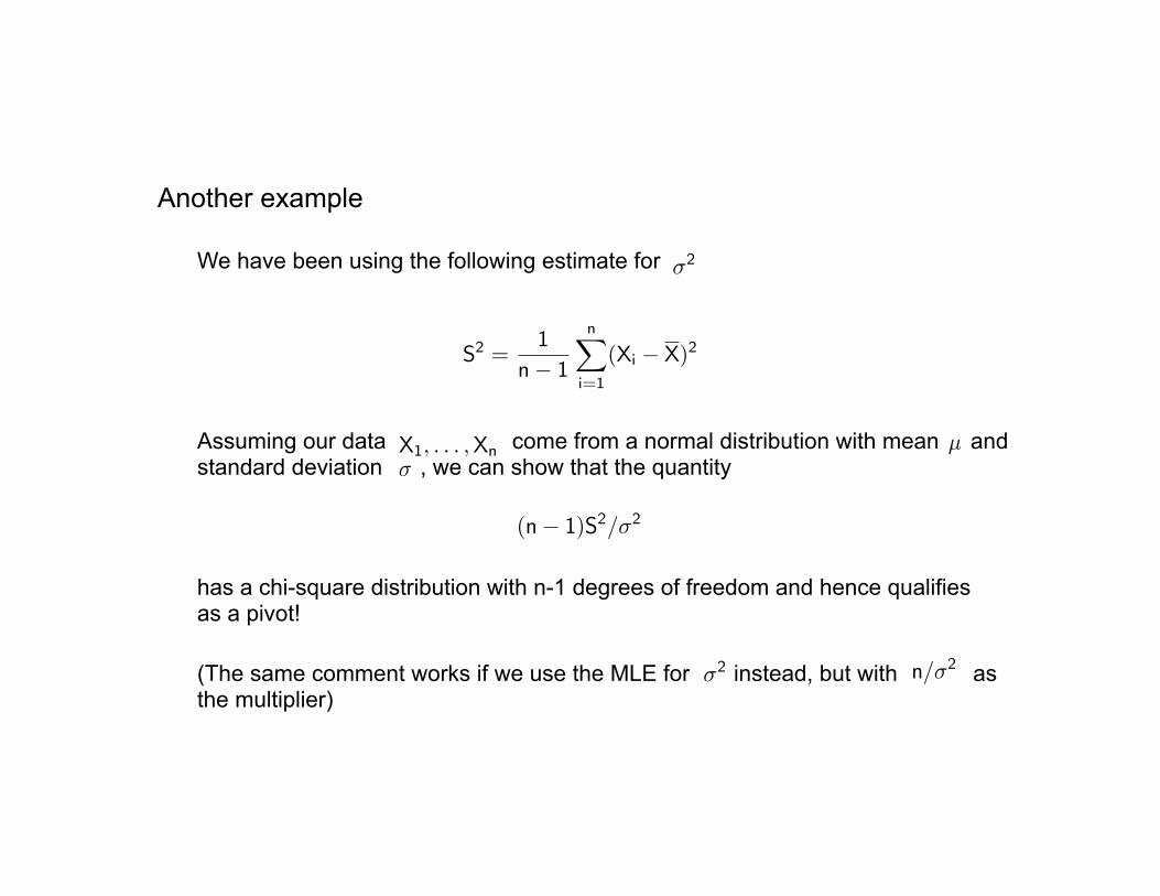
• Another example

• We have been using the following estimate for

• Assuming our data come from a normal distribution with mean and standard deviation , we can show that the quantity

• has a chi-square distribution with n-1 degrees of freedom and hence qualifies as a pivot!

• (The same comment works if we use the MLE for instead, but with as the multiplier)

S2 =1

n� 1

nX

i=1

(Xi � X)2

(n� 1)S2/�2

�2

X1, . . . ,Xn µ�

�2 n/�2

• Pivots

• Therefore, we can find values a and b such that

• where has a chi-square distribution with n-1 degrees of freedom

• Combining these two expressions we find

• and by inverting we derive a 95% confidence interval for

P(�2n�1 < a) = 0.025 and P(�2

n�1 > b) = 0.025

�2n�1

⇥(n� 1)b�2/b, (n� 1)b�2/a

⇤

P�a (n� 1)b�2/�2 b

�

�2

• Exact v. approximate sampling distributions

• In the last few slides, we have focused mainly on exact expressions for the sampling distribution of an estimator -- We have seen that the price of these “clean” results is a set of strong assumptions about how the data were generated

• And even when we are willing to make strong assumptions, it’s often the case that clean formula do not exist for the exact sampling distribution of an estimator -- Instead we have to rely on approximations

• Our starting point for these approximations comes from one of the properties we discussed last lecture, consistency...

• Exact v. approximate sampling distributions

• We let denote an estimator based on n samples -- We said that it was consistent if converges to the unknown value “in probability”

• Intuitively, this means that the errors get small as we collect more and more data -- As we have seen, however, there is tremendous value in not only knowing that the errors get small but in knowing how big they can be, their “typical” values

• These more refined statements mean we need to know something of the sampling distribution of our estimator -- And, in particular, can we say something approximate “in the limit” (that is general and maybe easier to work out mathematically) as opposed to something exact

b✓n X1, . . . ,Xnb✓n ✓⇤

b✓n � ✓⇤

• Convergence in distribution

• To make this precise, we say that a sequence of random variables and let denote the cumulative distribution function of -- Let Z be a random variable with CDF F

• We say that converges in distribution to Z if

• at all points where F is continuous -- We write

Z1,Z2, . . .Fn Zn

Z1,Z2, . . .

Fn(x) ! F(x)

ZnD! Z


• We can word consistency in terms of convergence in distribution as well -- We say that an estimator is consistent if converges in distribution to a “constant” random variable (that is a random variable that takes on the value with probability 1)

• The Central Limit Theorem is also a statement about convergence in probability -- That is, if are independent and identically distributed random variables with mean and variance , then their sample mean

• where Y has a normal distribution with mean 0 and variance

pn(Xn � µ)

D! Y

Xn, . . . ,Xnµ �2

�2

Xn

b✓n✓⇤✓⇤


• Informally, we say that the sample mean has approximately a normal distribution with mean and standard deviation “for large n” -- Or, more concisely, we say that is asymptotically normal

• This is an approximate version of the exact statement we examined at the beginning of this lecture, when our data really did come from a normal distribution

• Results such as these are the starting point for building “approximate” or “asymptotic” expressions for the sampling distribution of an estimate

Xnµ �/

pn

Xn, . . . ,Xn

Xn


• When reasoning about convergence results, Slutsky’s Theorem is a workhorse -- If g(z,y) is a function that is jointly continuous at every point of the form z,c for some fixed c, and if and (converges in probability to a constant c), then

• What this means is that

• or, that the limit of sums is the sum of the limits, etc.

ZnD! Z Yn

D! c

www.stat.umn.edu/geyer/old03/5102/notes/ci.pdf

Zn + YnD! Z+ c

YnZnD! cZ

Zn/YnD! Z/c, c 6= 0

g(Zn,Yn)D! g(Z, c)


• The plug-in principle, for example, makes use of this fact -- If we have an asymptotically normal estimate such that

• and if is any consistent estimate of , then

• which we can use to “plug-in” estimates and construct confidence intervals

b✓npn(b✓n � ✓⇤)

D! Normal (0, ⌧ 2)

b⌧n ⌧

b✓n � ✓⇤

b⌧n/pn

D! Normal (0, 1)

• Plug-in

• This is what we did when we considered

• as s is a consistent estimate of (see the end of this lecture for the details)

• Notice that Gosset worked out the exact sampling distribution for the plug-in estimate for small sample sizes n -- As n gets large, the effect of using s diminishes and, as we see here and on a previous slide, the whole thing approaches a normal distribution asymptotically

X� µ

s/pn

versusX� µ

�/pn

�

• Plug-in

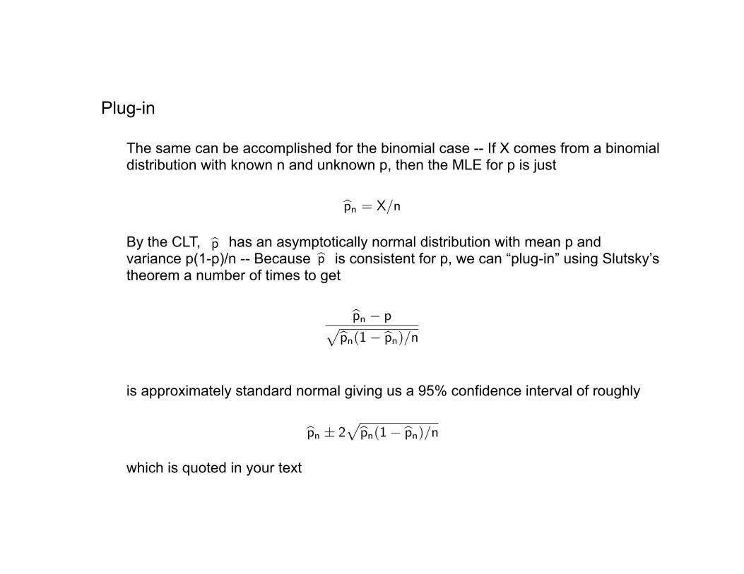
• The same can be accomplished for the binomial case -- If X comes from a binomial distribution with known n and unknown p, then the MLE for p is just

• By the CLT, has an asymptotically normal distribution with mean p and variance p(1-p)/n -- Because is consistent for p, we can “plug-in” using Slutsky’s theorem a number of times to get

• is approximately standard normal giving us a 95% confidence interval of roughly

• which is quoted in your text

bpbp

bpn = X/n

bpn � ppbpn(1� bpn)/n

bpn ± 2pbpn(1� bpn)/n

• Without plugging in

• Actually in this case, we can work things out without plugging in -- That is, by the CLT we know that

• is approximately normal so that

• By solving a quadratic equation we come up with the interval

• which agrees with our previous expression as n gets large (although this formula is rarely quoted in introductory texts)

bpn + 1n ± 2

q1n2 +

bpn(1�bpn)n

1+ 4n

P

�2

bpn � ppp(1� p)/n

2

!⇡ 0.95

bpn � ppp(1� p)/n

• Convergence in distribution: The MLE

• We can also say something quite general about Maximum Likelihood Estimates -- Recall the likelihood and log-likelihood functions

• If we let be the MLE (and there are technical conditions we won’t fuss about now) then not only is a consistent estimate of , it is also asymptotically normal

L(✓) =nY

i=1

f(Xi|✓) and l(✓) = logL(✓) =nX

i=1

log f(Xi|✓)

b✓nb✓n ✓⇤


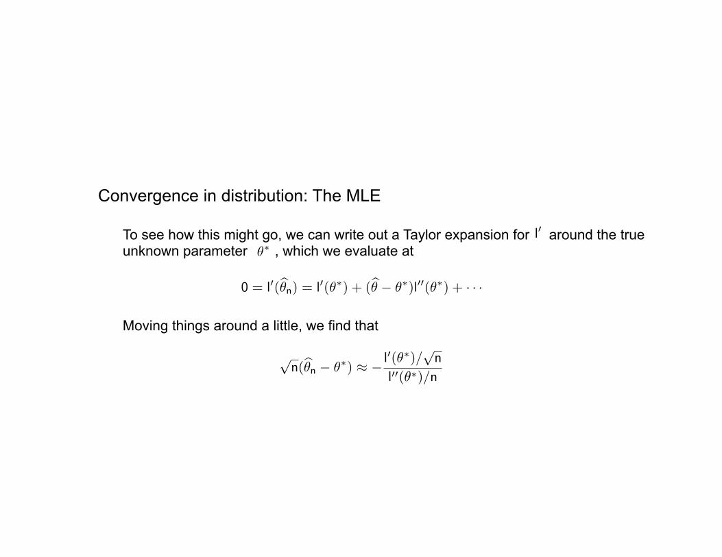
• To see how this might go, we can write out a Taylor expansion for around the true unknown parameter , which we evaluate at

• Moving things around a little, we find that

0 = l0(b✓n) = l0(✓⇤) + (b✓ � ✓⇤)l00(✓⇤) + · · ·

✓⇤l0

pn(b✓n � ✓⇤) ⇡ � l0(✓⇤)/

pn

l00(✓⇤)/n


• We can treat the limits in the upstairs and downstairs separately and apply Slutsky’s theorem -- For example, the downstairs looks like an average

• This can be shown to converge to a constant known as the expected Fisher Information -- It is given by the expression

•

I(✓) = �E✓

@2

@2✓f(X|✓)

�

l00(✓)/n =1

n

nX

i=1

@2

@2✓f(Xi|✓)


• When the dust settles on our calculations, under certain regularity conditions and for large n, the MLE is asymptotically normal with mean and standard deviation or that

• has a standard normal distribution for large n

• Now, following the plug-in principle (applying Slutsky’s theorem), we can substitute the estimate for in the standard deviation to come up with approximate 95% confidence intervals of the form

1/pnI(✓⇤)

b✓n � ✓⇤

1/pnI(✓⇤)

✓⇤b✓n

b✓n ✓⇤

b✓n ±2q

nI(b✓n)

• Our approach

• I present this material mainly for pedagogical reasons -- This way you see how confidence intervals are derived analytically, pushing through various limit theorems to establish “large n” approximate results

• Instead of dealing in formulae, we will rely on R or some other bootstrap-enlightened software package to provide us with ready assessments of precision or confidence intervals computationally

• For the most part, when a formula exists, the bootstrap will agree with it, making it (perhaps) a more general tool for you as you venture out into the world...

•

Real world


Sample n times from

Observed sample

Estimate

✓⇤

f(x|✓⇤)

X1, . . . ,Xn

Bootstrap world

Bootstrap world parameter

Sample n times from

Bootstrap sample

Bootstrap replicate

b✓

f(x|b✓)

eX1, . . . , eXn

b✓ = s(X1, . . . ,Xn) e✓ = s(eX1, . . . , eXn)

Bootstrap world


Sample n times from

Bootstrap sample

Bootstrap replicate

b✓

f(x|b✓)

eX1, . . . , eXn

e✓ = s(eX1, . . . , eXn) e✓1

Bootstrap world


Sample n times from

Bootstrap sample

Bootstrap replicate

b✓

f(x|b✓)

eX1, . . . , eXn

e✓ = s(eX1, . . . , eXn)

Bootstrap world


Sample n times from

Bootstrap sample

Bootstrap replicate

b✓

f(x|b✓)

eX1, . . . , eXn

e✓ = s(eX1, . . . , eXn)

Bootstrap world


Sample n times from

Bootstrap sample

Bootstrap replicate

b✓

f(x|b✓)

eX1, . . . , eXn

e✓ = s(eX1, . . . , eXn)

Bootstrap world


Sample n times from

Bootstrap sample

Bootstrap replicate

b✓

f(x|b✓)

eX1, . . . , eXn

e✓ = s(eX1, . . . , eXn)

e✓2

e✓3

e✓4

e✓5

• The bootstrap

• If we repeat this process B times, we form B bootstrap replicates from which we can estimate the sampling distribution of -- Plotting these B values (a histogram, say) gives us information about the performance of our estimator

b✓

• The bootstrap

• Bias: Let’s let (horrible notation) denote the mean of the B bootstrap samples

• Recalling that our estimate plays the role of in the bootstrap world, we can estimate the bias in with

• Standard error: We can estimate with the sample standard deviation of the bootstrap replicates

✓⇤

se(b✓)

e✓ =1

B

BX

b=1

e✓b

b✓b✓

e✓

e✓ � b✓

vuut 1

B� 1

BX

b=1

(e✓b � e✓)2seboot

=

• The bootstrap

• We can then form confidence intervals either by

• if our bootstrap replicates look reasonably normal, or by using directly the 0.025 and 0.975 quantiles of the bootstrap replicates as our end points

• This latter scheme is called the percentile bootstrap confidence interval and is pretty easy to work with -- It is intuitive and will work reasonably well even if there your bootstrap distribution suggests things are skewed

b✓ ± 2 seboot

lecture 10: pivot - ucla statistics | websitecocteau/stat105/lectures/lecture10.pdflecture 10: pivot...

Documents