lecture 10 - university of...
TRANSCRIPT

Lecture 10Lecture 10
The Dirac equationThe Dirac equation
WS2010/11WS2010/11: : ‚‚Introduction to Nuclear and Particle PhysicsIntroduction to Nuclear and Particle Physics‘‘
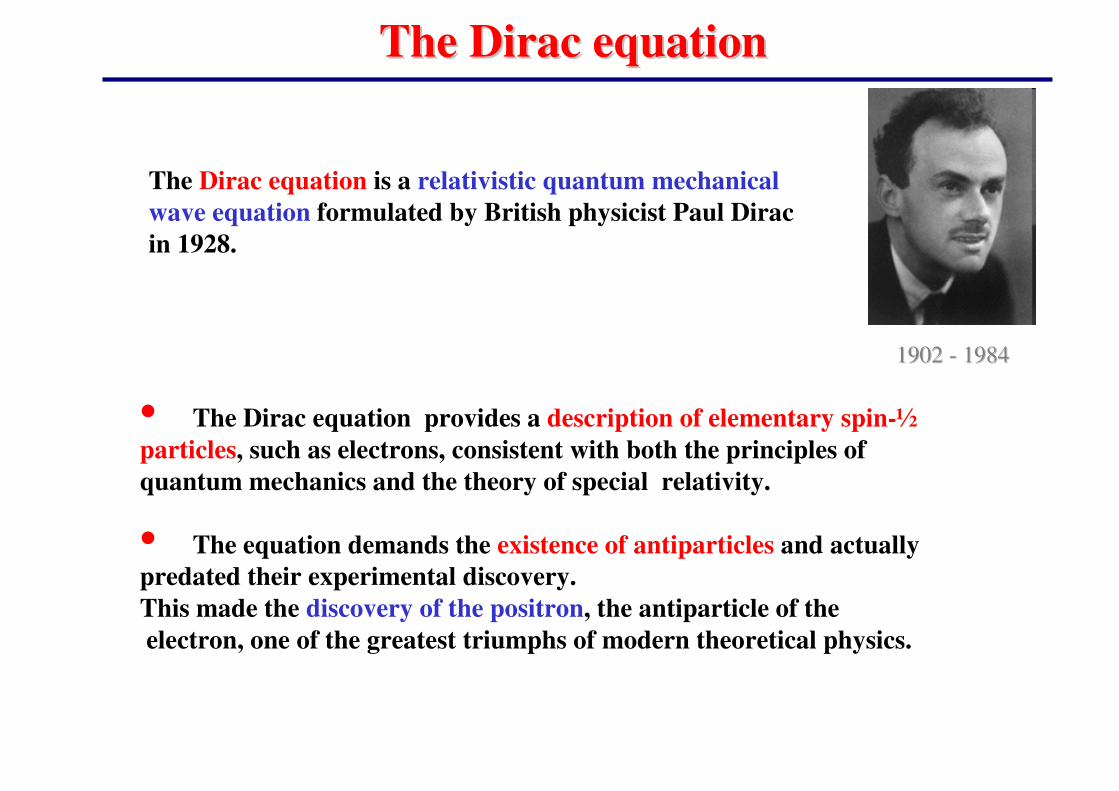
The Dirac equation is a relativistic quantum mechanical
wave equation formulated by British physicist Paul Dirac
in 1928.
The Dirac equationThe Dirac equation
• The Dirac equation provides a description of elementary spin-½
particles, such as electrons, consistent with both the principles of
quantum mechanics and the theory of special relativity.
• The equation demands the existence of antiparticles and actually
predated their experimental discovery.
This made the discovery of the positron, the antiparticle of the
electron, one of the greatest triumphs of modern theoretical physics.
1902 1902 -- 19841984
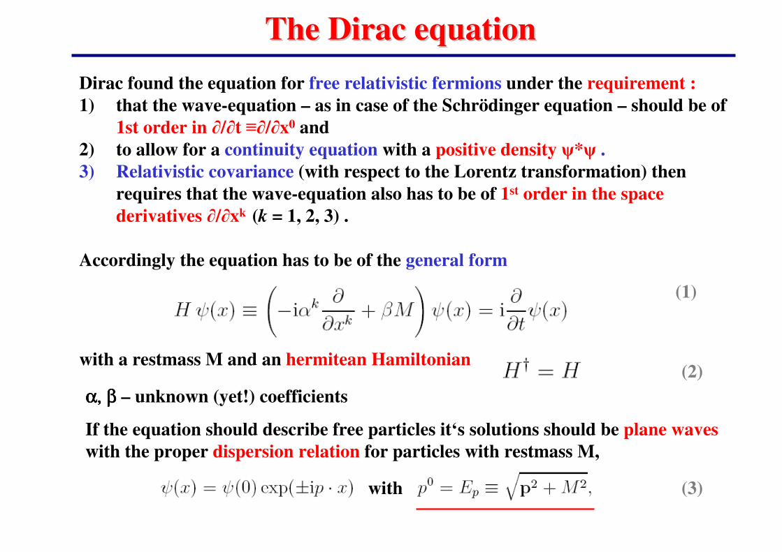
Dirac found the equation for free relativistic fermions under the requirement :
1) that the wave-equation – as in case of the Schrödinger equation – should be of
1st order in �/�t ��/�x0 and
2) to allow for a continuity equation with a positive density �*� .
3) Relativistic covariance (with respect to the Lorentz transformation) then
requires that the wave-equation also has to be of 1st order in the space
derivatives �/�xk (k = 1, 2, 3) .
Accordingly the equation has to be of the general form
The Dirac equationThe Dirac equation
(1)
(2)with a restmass M and an hermitean Hamiltonian
α, βα, βα, βα, β – unknown (yet!) coefficients
If the equation should describe free particles it‘s solutions should be plane waves
with the proper dispersion relation for particles with restmass M,
(3)with

The Dirac equation The Dirac equation
(4)
(5)
By comparing the quadratic form of (1), symmetrized in the indices k, l ,
with the Klein-Gordon-equation (4)
one has to require that the unknown coefficients �k (k = 1, 2, 3) and �
must have the properties
(6)
(7)
The conditions (6) can only be fulfilled for matrices. Due to Eq. (2) these
matrices have to be hermetian:
The eigenvalues then are real and according to (6) can only be +1 .
In this case the wavefunction � (or each component of �) has to be a solution also
of the Klein-Gordon-Equation:

The Dirac equation The Dirac equation
These matrices must be traceless. Accordingly, the dimension of the matrices
has to be an even number. In 2 dimensions, however, there are only 3 linearly
independent matrices that anticommute, i.e. the Pauli matrices:
(9)
(10)
or unitary transformations of (10). Accordingly, the �k, � must be at least 4x4
matrices. In Pauli-Dirac standard notation (with 2x2 submatrices) these are
given by
(11)
Unitary equivalent representations are also possible.
(8)
Furthermore, since �k = −��k� – due to cyclic invariance of the trace ����
The Dirac equation The Dirac equation
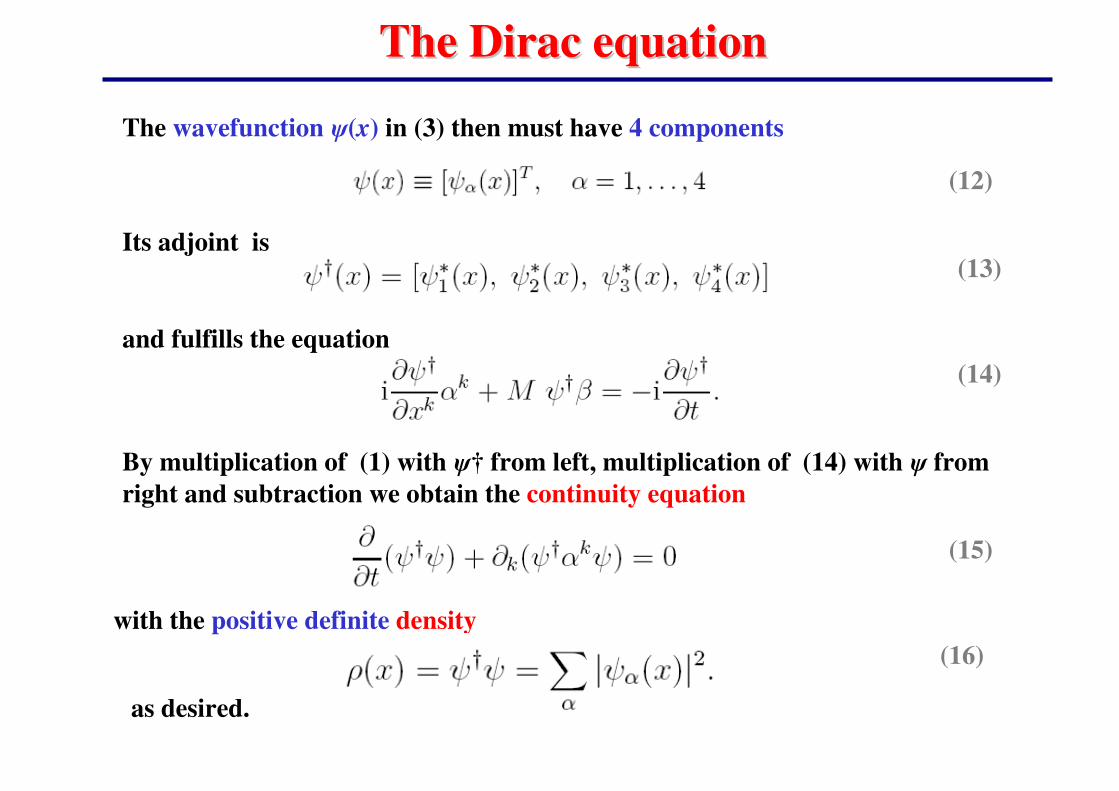
The wavefunction �(x) in (3) then must have 4 components
(12)
Its adjoint is
and fulfills the equation
(13)
(14)
By multiplication of (1) with �† from left, multiplication of (14) with � from
right and subtraction we obtain the continuity equation
(15)
with the positive definite density
(16)
as desired.

�-matrices and Dirac-algebra
For the analysis of transformation properties it is more convenient to introduce
an equivalent set of matrices which is obtained as follows:
(17)
(18)
The Dirac-equation then reads:.
with the Pauli-adjoint Spinor(19)
(20)
(21)
For the �-matrices Eqs. (6)
then become more compact:
and Eq. (7) leads to the pseudo-hermeticity
�-matrices and Dirac-algebra
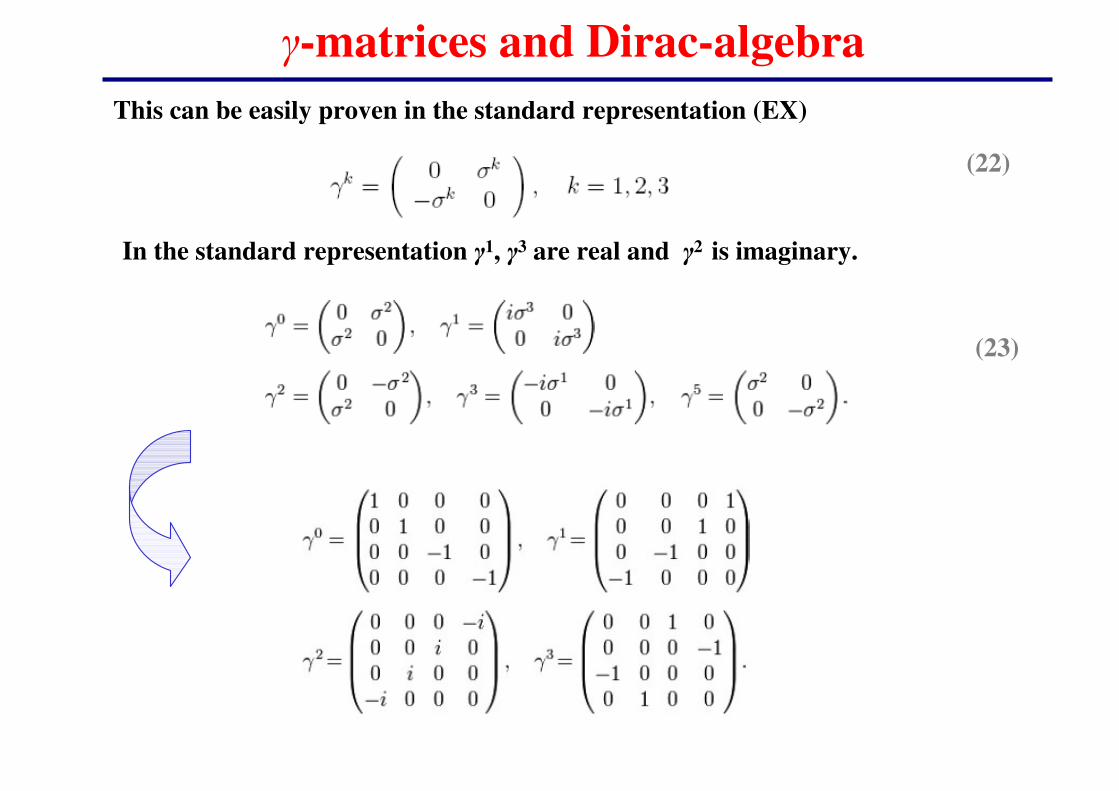
This can be easily proven in the standard representation (EX)
(22)
(23)
In the standard representation �1, �3 are real and �2 is imaginary.

and describes the vanishing of the four-divergence of the four-current j�(x).
With the help of the 4-� matrices one can construct a complete set of 4x4
matrices.
Since a general 4x4 has 16 independent elements there also have to be 16 basis
elements. For convenience one chooses the basis:
�-matrices and Dirac-algebra
(23)
The continuity equation (15) then reads (EX)
1 matrix (4 x4 unit matrix)
4 matrixes
6 matrixes (antisymmetric)
4 matrixes
1 matrix
(24)
with

�-matrices and Dirac-algebra
where �5 is the ‚chirality‘ matrix given by
(25)
This matrix can also be written as
(26)
(27)if (µ,ν,ρ,σ)(µ,ν,ρ,σ)(µ,ν,ρ,σ)(µ,ν,ρ,σ) is an even permutation of (0,1,2,3)
if (µ,ν,ρ,σ)(µ,ν,ρ,σ)(µ,ν,ρ,σ)(µ,ν,ρ,σ) is an odd permutation of (0,1,2,3)
in all other cases
if (µ,ν,ρ,σ)(µ,ν,ρ,σ)(µ,ν,ρ,σ)(µ,ν,ρ,σ) is an even permutation of (0,1,2,3)
if (µ,ν,ρ,σ)(µ,ν,ρ,σ)(µ,ν,ρ,σ)(µ,ν,ρ,σ) is an odd permutation of (0,1,2,3)
in all other cases
with the complete antisymmetric unit tensor of fourth order.
The matrix �5 has the properties (EX)
(28)

�-matrices and Dirac-algebra
(29)
The nonzero elements of the matrices �µνµνµνµν are those from nondiagonal spacial
components (�, �) = (k, l) with k unequal l and (�, �) = (0, k). These elements can
be expressed as
(30)
(31)where
(32)
(33)
is the ε ε ε ε -tensor in 3 dimensions.
The three 4x4 matrices (29) have the properties of a set of spin-matrices,
i.e (EX)
which is proven explicitly in the standard representation
�-matrices and Dirac-algebra
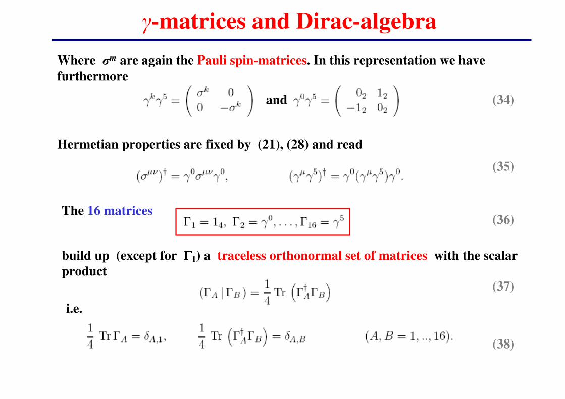
Where �m are again the Pauli spin-matrices. In this representation we have
furthermore
(34)
Hermetian properties are fixed by (21), (28) and read
The 16 matrices
(35)
(36)
build up (except for ΓΓΓΓ1) a traceless orthonormal set of matrices with the scalar
product
(37)
i.e.
(38)
and

�-matrices and Dirac-algebra
(39)
In particular, these matrices are linearly independent.
Accordingly any 4x4 matrix M can be written as a linear combination in the
basis (36):
Products of arbitrary matrices thus may also be written in terms of an
expansion in the ΓΓΓΓ-matrices.
For a couple of such products we present the result in the following
‚multiplication table‘:

�-matrices and Dirac-algebra
(40)
�-matrices and Dirac-algebra
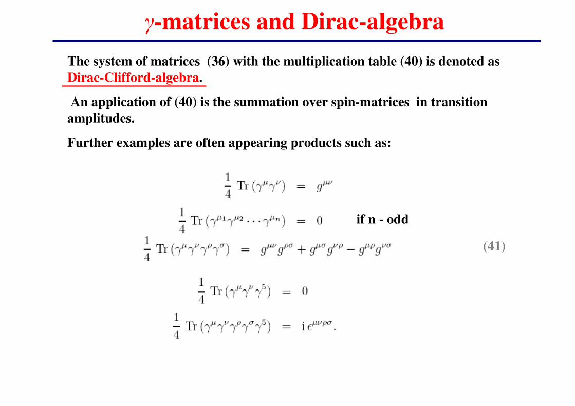
(41)
The system of matrices (36) with the multiplication table (40) is denoted as
Dirac-Clifford-algebra.
An application of (40) is the summation over spin-matrices in transition
amplitudes.
Further examples are often appearing products such as:
if n - odd
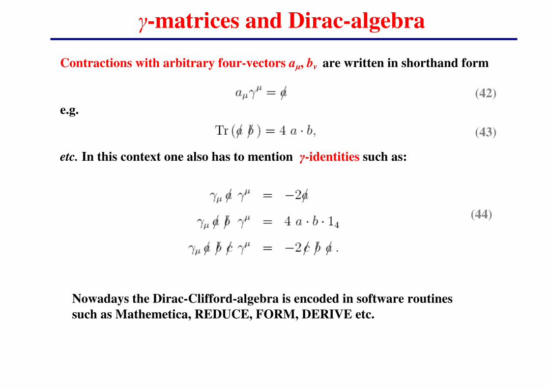
Contractions with arbitrary four-vectors a�, bv are written in shorthand form
e.g.
etc. In this context one also has to mention �-identities such as:
�-matrices and Dirac-algebra
(42)
(43)
(44)
Nowadays the Dirac-Clifford-algebra is encoded in software routines
such as Mathemetica, REDUCE, FORM, DERIVE etc.
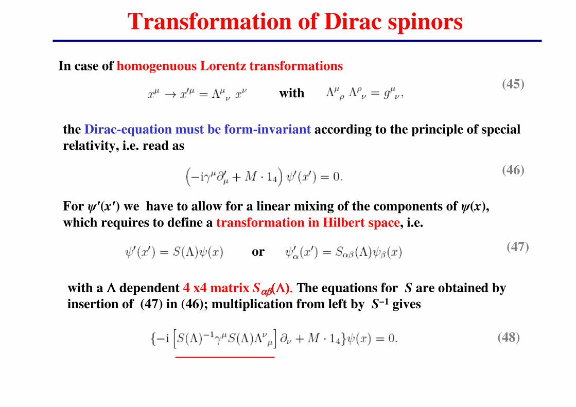
Transformation of Dirac spinors
(45)
In case of homogenuous Lorentz transformations
the Dirac-equation must be form-invariant according to the principle of special
relativity, i.e. read as
(46)
(47)
For ��(x�) we have to allow for a linear mixing of the components of �(x),
which requires to define a transformation in Hilbert space, i.e.
or
with
with a ΛΛΛΛ dependent 4 x4 matrix Sαβαβαβαβ((((ΛΛΛΛ)))).... ΤΤΤΤhe equations for S are obtained by
insertion of (47) in (46); multiplication from left by S−1 gives
(48)
Transformation of Dirac spinors
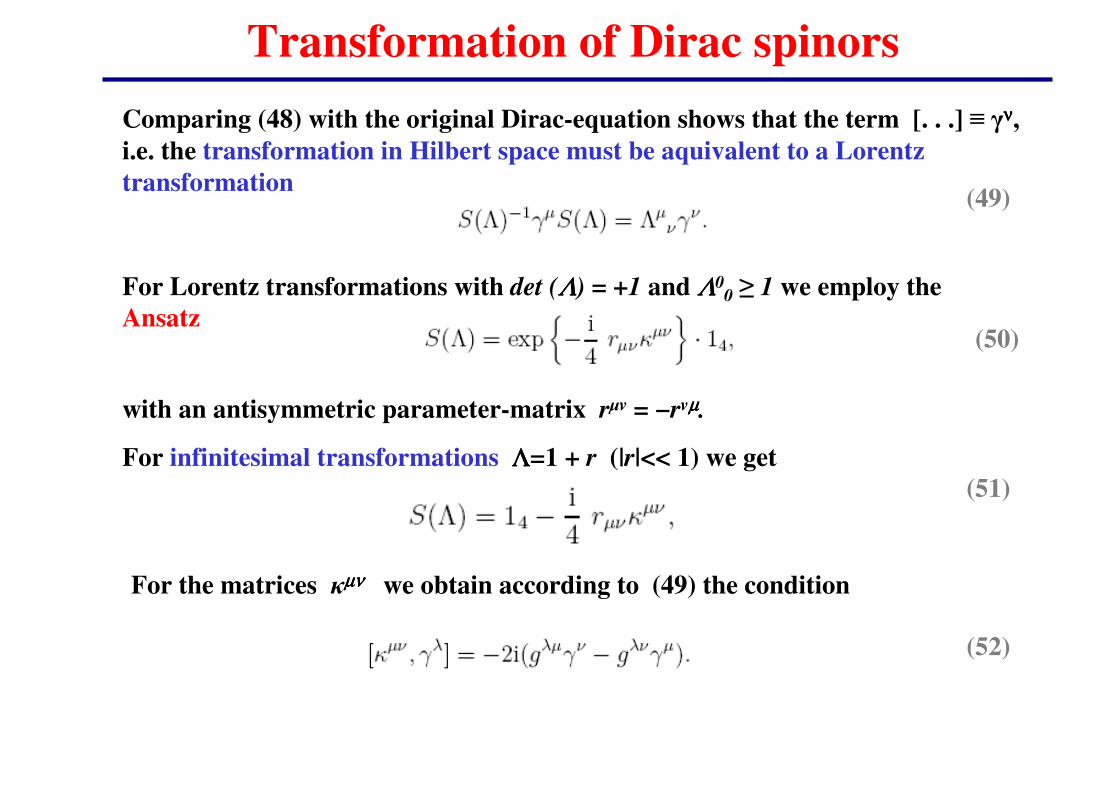
Comparing (48) with the original Dirac-equation shows that the term [. . .] � �νννν,
i.e. the transformation in Hilbert space must be aquivalent to a Lorentz
transformation (49)
For Lorentz transformations with det (ΛΛΛΛ) = +1 and ΛΛΛΛ00 � 1 we employ the
Ansatz(50)
with an antisymmetric parameter-matrix r�v = −rvµµµµ.
For infinitesimal transformations ΛΛΛΛ=1 + r (|r|<< 1) we get
(51)
(52)
For the matrices µνµνµνµν we obtain according to (49) the condition

Transformation of Dirac spinors
Using the multiplication table (40) one identifies the unique solution
(53)
A four-component field function �αααα(x), which transforms under homogeneous
Lorentz transformations (47) as
is called a Dirac-Spinor.
The 4x4 matrices S(ΛΛΛΛ) – acting in the Hilbert space – follow:
(54)
(55)
The group transformations are not unitary, but due to the real and antisymmetric
parameter-matrix r�v follow:
(56)

Transformation of Dirac spinors
We now consider (54) in particular for rotations and Lorentz boosts for which we
obtain:
for a rotation with vector
for a boost with velocity
An expansion of the exp.-function (54) and using the matrix identities (40) gives:
(57)
(58)
1) For arbitrary complex vectors a,b a pure rotation leads to a
unitary transformation (with )
Transformation of Dirac spinors
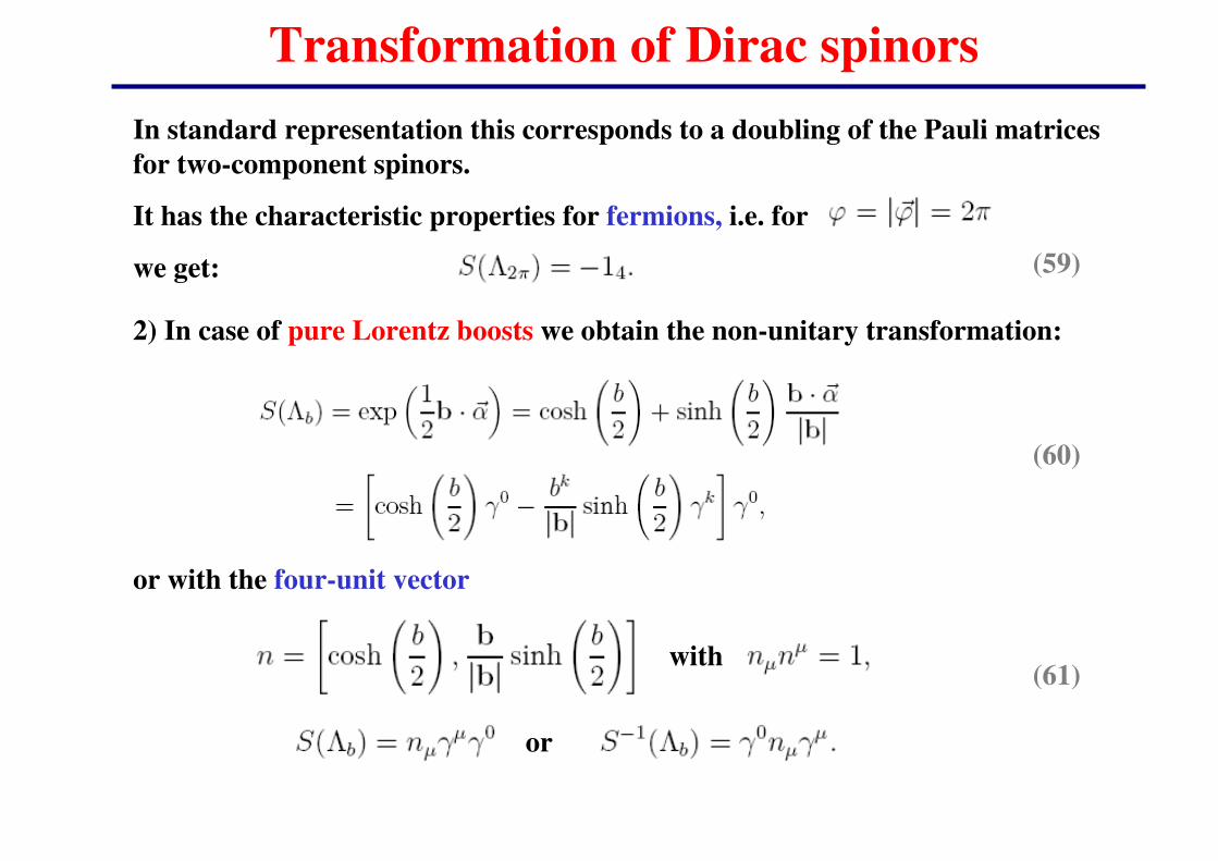
In standard representation this corresponds to a doubling of the Pauli matrices
for two-component spinors.
It has the characteristic properties for fermions, i.e. for
we get: (59)
2) In case of pure Lorentz boosts we obtain the non-unitary transformation:
(60)
or with the four-unit vector
(61)with
or

Transformation of Dirac spinors
For parity transformations we have to allow for a phase � = ±1 (� is the eigenvalue
of the parity transformation) as in case of the Klein-Gordon field . The condition
(49) ( ) leads to:
(62)
which is solved by (63)
Eq. (47) then reads:(64)
���� The Dirac equation is form-invariant under these parity transformations.
For the particular matrix �5 this implies:
(65)
whereas – due to the matrices �µνµνµνµν - one finds:
(66)
Transformation of Dirac spinors
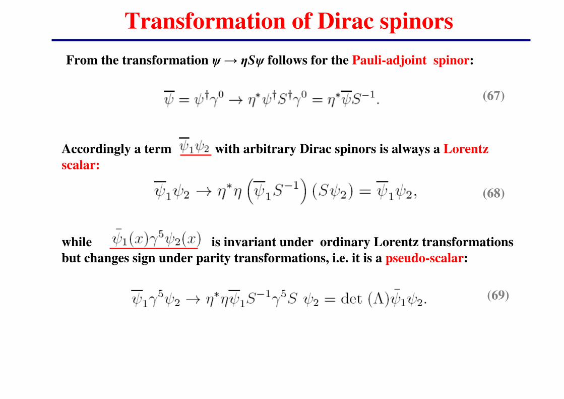
From the transformation � � S� follows for the Pauli-adjoint spinor:
(67)
Accordingly a term with arbitrary Dirac spinors is always a Lorentz
scalar:
(68)
while is invariant under ordinary Lorentz transformations
but changes sign under parity transformations, i.e. it is a pseudo-scalar:
(69)
Transformation of Dirac spinors
scalar
4-vector
tensor of 2nd order
pseudovector
pseudoscalar
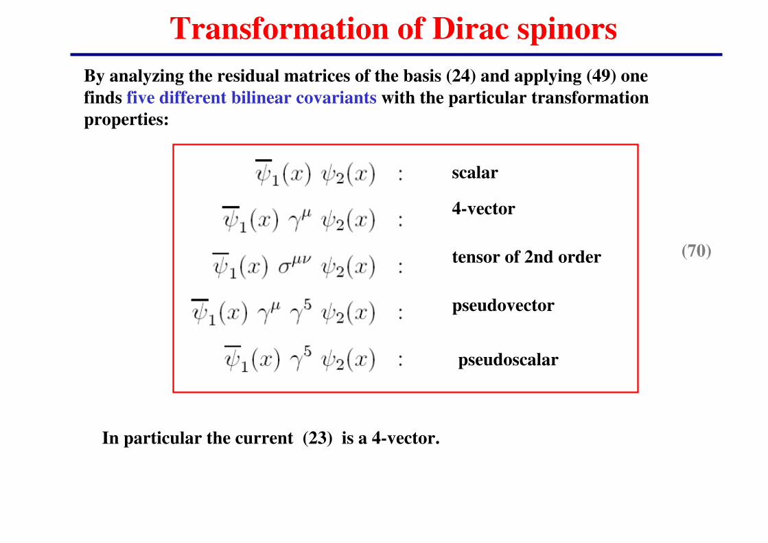
In particular the current (23) is a 4-vector.
By analyzing the residual matrices of the basis (24) and applying (49) one
finds five different bilinear covariants with the particular transformation
properties:
(70)

Solution of the free Dirac equation
The solution of the Dirac equation are plane waves (3).
In order to find the yet unknown spinors �(0) (or a suitable basis) we consider
solutions for positive and negative energies, separately:
with
(71)
By insertion in Eq. (1) we obtain:
(72)
(73)or in �-notation:
In order to specify the spinors u and υυυυ we consider first the case p = 0 (i.e. we
evaluate the spinor in the rest frame of the particle). In this frame (73) reads:
(74)

Solution of the free Dirac equation
(75)
Now we can choose for u(0) and υυυυ(0) two orthogonal eigenspinors to �0 with
eigenvalues +1 and −1 , which are denoted by .
Since Tr (�0) = 0 each eigenvalue appears twice. Furthermore, the matrices
(29) commute with �0 and we can choose ur(0) and υυυυr(0) as eigenspinors of
with eigenvalues s= +1, where aa is an arbitrary unit vector because according to
(57) we have :
In standard representation one chooses a = (0, 0, 1) which leads to
(76)
The 4 basis spinors are normalized according to:
(77)
Accordingly we get the orthogonality relation:
(78)
since u and υυυυ belong to different eigenvalues of �0 .
Solution of the free Dirac equation
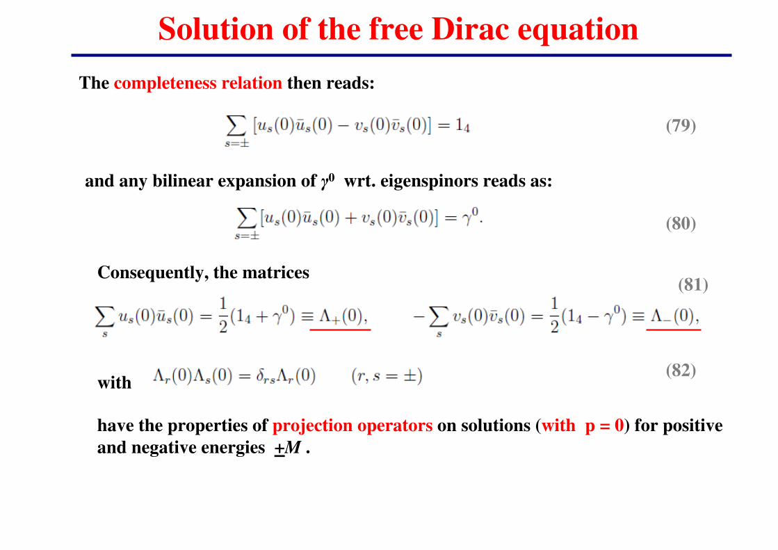
The completeness relation then reads:
(79)
and any bilinear expansion of �0 wrt. eigenspinors reads as:
(80)
Consequently, the matrices
with
(81)
(82)
have the properties of projection operators on solutions (with p = 0) for positive
and negative energies +M .

Solution of the free Dirac equation
In standard representation these relations become immediately apparent:
(83)
(84)
and the 4x4 matrices read
In order to get solutions for we have to apply a Lorentz transformation,
i.e. the transformation (61) with the proper Lorentz boost:
(85)
The appropriate boost velocity is given by:
(86)

Solution of the free Dirac equation
According to (60) one gets with the parameters of (61) :
and
with
(87)
(88)
The solution is according to (60), (61):
(89)
Now the spinors for Dirac particles with momentum p read:
(90)
Solution of the free Dirac equation
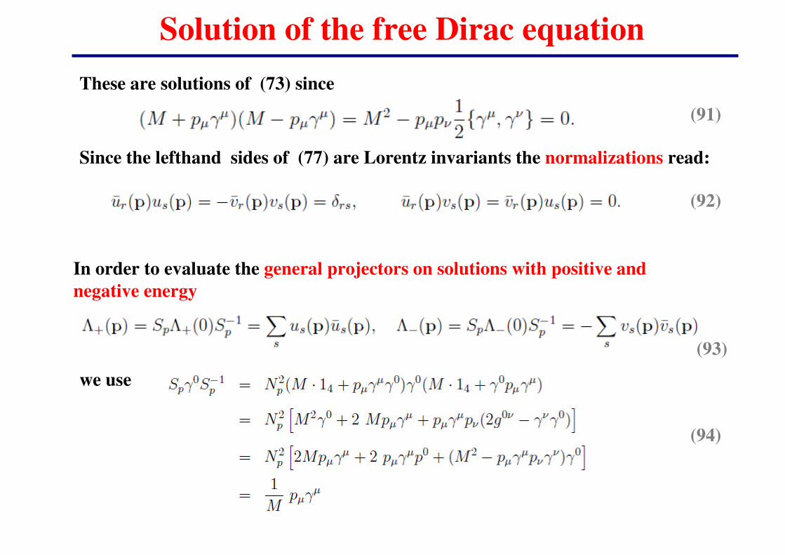
These are solutions of (73) since
(91)
Since the lefthand sides of (77) are Lorentz invariants the normalizations read:
(92)
In order to evaluate the general projectors on solutions with positive and
negative energy
(93)
we use
(94)

Solution of the free Dirac equation
and obtain (EX)(95)
(96)
The completeness relation (79) then reads:
Note: the eigenvalue equation (76) does not hold for finite p, since ΣΣΣΣ3 does not
commute with Sp .
In standard representation the 4 basis spinors are given by:
(97)
or explicitly:
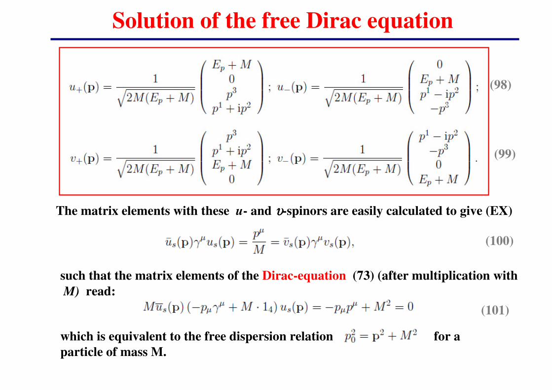
Solution of the free Dirac equation
(98)
(99)
The matrix elements with these u- and υυυυ-spinors are easily calculated to give (EX)
(100)
such that the matrix elements of the Dirac-equation (73) (after multiplication with
M) read:
(101)
which is equivalent to the free dispersion relation for a
particle of mass M.

Solution of the free Dirac equation
(102)
In the representation (100) – in the nonrelativistic limit |p| << M – the lower
components of us become smaller by a factor |p|/(2M) than the upper
components, while for υυυυs the relations are opposite.
The relation between us and υυυυs may be expressed according to (25) as (EX):
i.e. the chirality matrix �5 exchanges u- and υυυυ-spinors.
Finally, the explicit form of the Lorentz boost for the transformation (85) reads
(using NE = M(Ep +M)) (EX):
(103)