lecture 11 : glassy dynamics - intermediate …upmc.fr atomic modeling of glass – lecture 11...
TRANSCRIPT
[email protected] Atomic modeling of glass – LECTURE 11 DYNAMICS
LECTURE 11 : GLASSY DYNAMICS- Intermediate scattering function- Mean square displacement and beyond- Dynamic heterogeneities- Isoconfigurational Ensemble- Energy landscapes
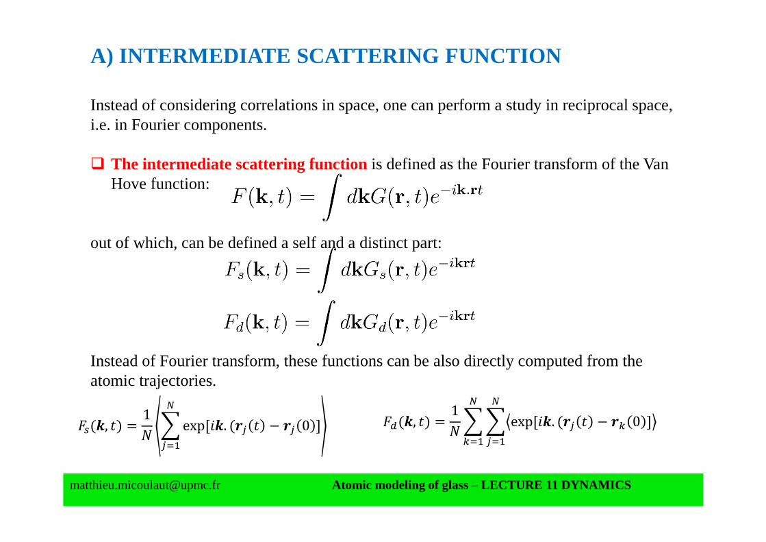
A) INTERMEDIATE SCATTERING FUNCTION
Instead of considering correlations in space, one can perform a study in reciprocal space, i.e. in Fourier components.
The intermediate scattering functionis defined as the Fourier transform of the Van Hove function:
out of which, can be defined a self and a distinct part:
Instead of Fourier transform, these functions can be also directly computed from the atomic trajectories.
(, ) =1 exp[. ( − 0 ]
(, ) =
1 exp[. ( − 0 ]
[email protected] Atomic modeling of glass – LECTURE 11 DYNAMICS
(, ) =1 exp[. ( − 0 ]
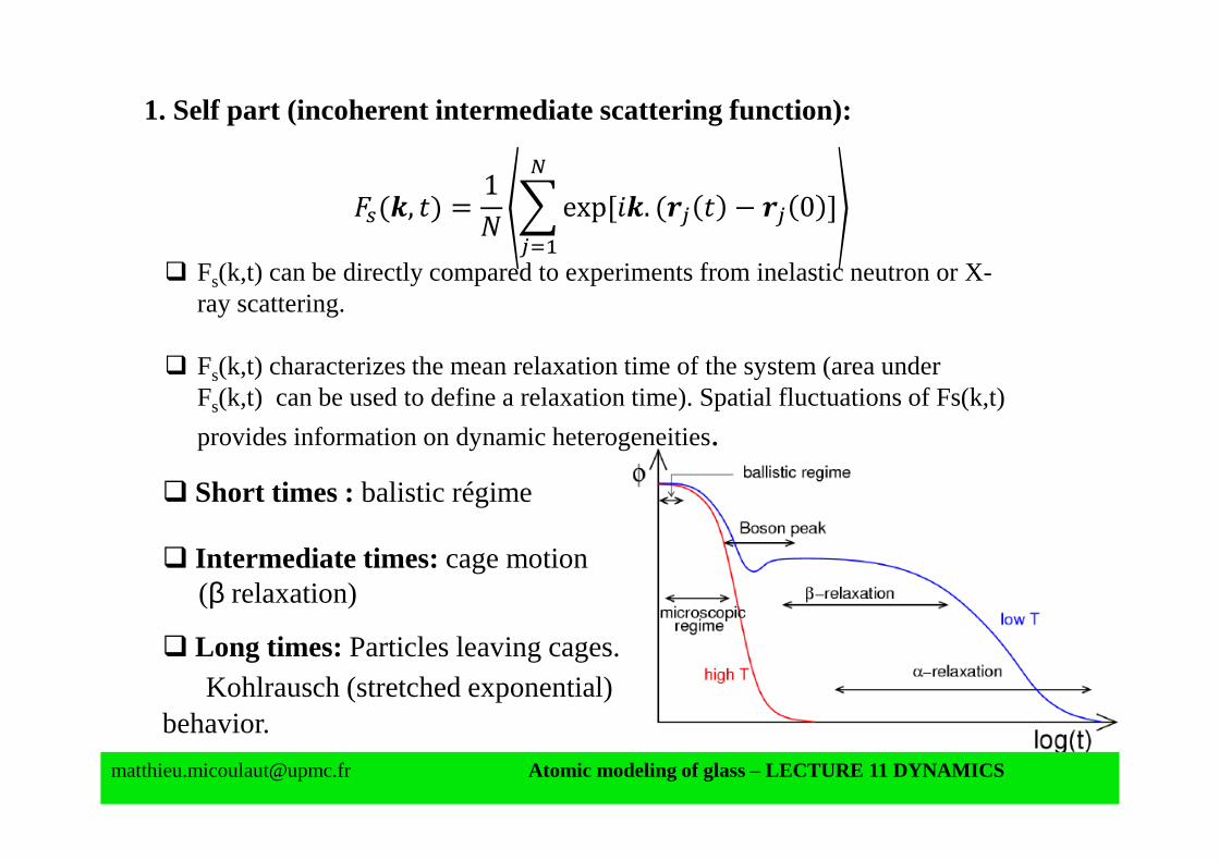
1. Self part (incoherent intermediate scattering function):
Fs(k,t) can be directly compared to experiments from inelastic neutron or X-ray scattering.
Fs(k,t) characterizes the mean relaxation time of the system (area underFs(k,t) can be used to define a relaxation time). Spatial fluctuations of Fs(k,t)
provides information on dynamic heterogeneities.
Short times : balistic régime
Intermediate times: cage motion (β relaxation)
Long times: Particles leaving cages. Kohlrausch (stretched exponential)
behavior.
[email protected] Atomic modeling of glass – LECTURE 11 DYNAMICS

Examples : CaAl2SiO8
Tm=2000 K
Morgan and Spera, GCA 2001
Cage motion (β régime) extends to long times at lowT Horbach, Kob PRB 1999
[email protected] Atomic modeling of glass – LECTURE 11 DYNAMICS
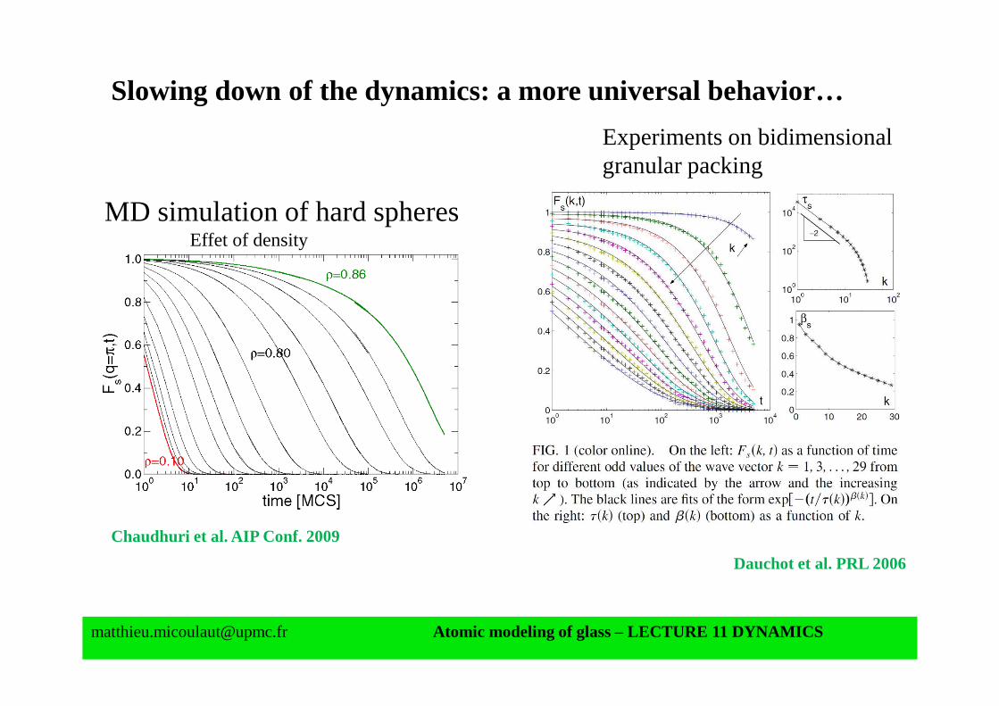
Slowing down of the dynamics: a more universal behavior…
Chaudhuri et al. AIP Conf. 2009
MD simulation of hard spheresEffet of density
Experiments on bidimensionalgranular packing
Dauchot et al. PRL 2006
[email protected] Atomic modeling of glass – LECTURE 11 DYNAMICS

2. Distinct part (coherent intermediate scattering function):
(, ) =1 exp[. ( − 0 ]
Fd(k,t) can be measured in coherent inelastic neutron or x-ray scattering
experiments (k=kinitial-kfinal).
Fluctuations of Fd(k,t) give information about dynamical heterogeneities.
Kob, 2000
[email protected] Atomic modeling of glass – LECTURE 11 DYNAMICS
0 0
tt
As2Se3
Bauchy et al., PRL 2013 Kob PRE 2000
A-B Lennard-Jones liquid
[email protected] Atomic modeling of glass – LECTURE 11 DYNAMICS
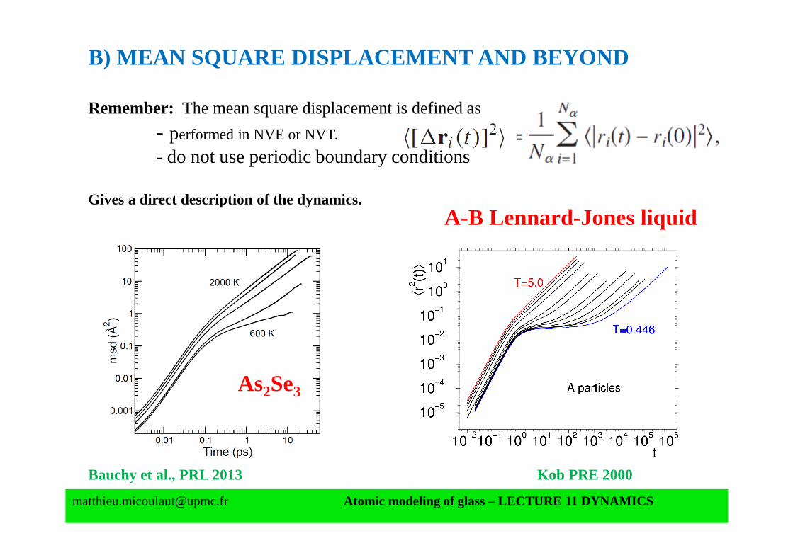
B) MEAN SQUARE DISPLACEMENT AND BEYOND
Remember: The mean square displacement is defined as
- performed in NVE or NVT.
- do not use periodic boundary conditions
Gives a direct description of the dynamics.
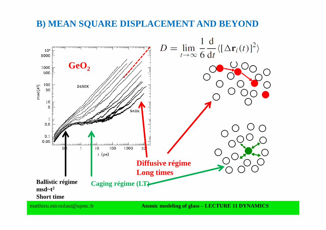
GeO2
Caging régime (LT)Ballistic régimemsd~t2
Short time
Diffusive régimeLong times
[email protected] Atomic modeling of glass – LECTURE 11 DYNAMICS
B) MEAN SQUARE DISPLACEMENT AND BEYOND
B) MEAN SQUARE DISPLACEMENT AND BEYOND
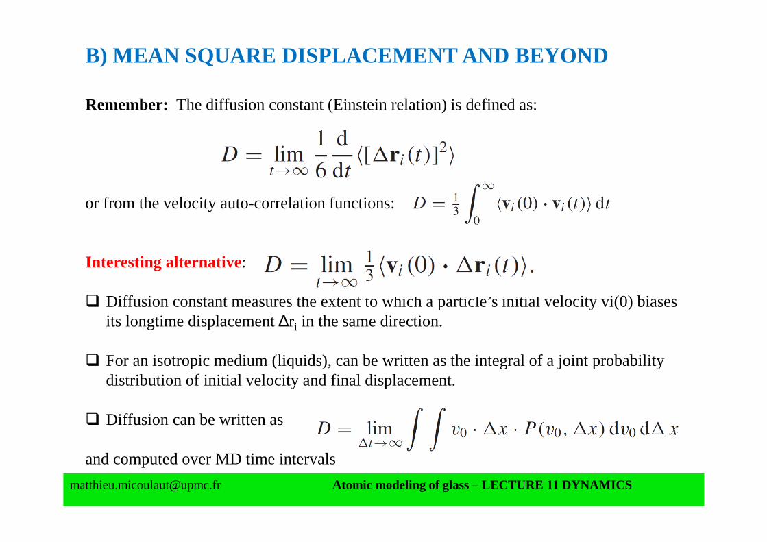
Remember: The diffusion constant (Einstein relation) is defined as:
or from the velocity auto-correlation functions:
Interesting alternative:
Diffusion constant measures the extent to which a particle’s initial velocity vi(0) biases its longtime displacement ∆ri in the same direction.
For an isotropic medium (liquids), can be written as the integral of a joint probability distribution of initial velocity and final displacement.
Diffusion can be written as
and computed over MD time intervals
[email protected] Atomic modeling of glass – LECTURE 11 DYNAMICS
A) MEAN SQUARE DISPLACEMENT AND BEYOND
At short times (hot liquid), the ballistic motion of particles is not spatially correlated(Maxwell-Boltzmann distribution f(v)).
At very long times (low temperature), particles lose memory of their original positions and velocities, and any spatial heterogeneity in the displacements is simply averaged out.
The presence of dynamic heterogeneity implies the existence of an intermediate time scale, dependent on the temperature, which reveals clustering in terms of particle mobility.
For purely random diffusion, one has (solution of Fick’s law):
[email protected] Atomic modeling of glass – LECTURE 11 DYNAMICS
[email protected] Atomic modeling of glass – LECTURE 11 DYNAMICS
B) MEAN SQUARE DISPLACEMENT AND BEYOND
At short times (hot liquid), since one has a Maxwell-Boltzmann distribution f(v) and also ∆r i=vi∆t, P is also Gaussian.
For moderate to deeply supercooled liquids, the intermediate-time behaviour of P becomes substantially non-Gaussian, reflecting the effects of ‘caged’ particles and the presence of dynamic heterogeneity.
Reflected in a non-Gaussian parameter
For a truly Gaussian distribution in r i, α2 =0
α2 (0)=0 and for
[email protected] Atomic modeling of glass – LECTURE 11 DYNAMICS
B) MEAN SQUARE DISPLACEMENT AND BEYOND
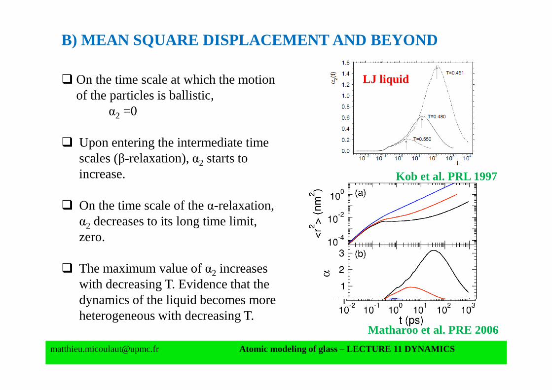
LJ liquid
Kob et al. PRL 1997
On the time scale at which the motion of the particles is ballistic,
α2 =0
Upon entering the intermediate time scales (β-relaxation), α2 starts to increase.
On the time scale of the α-relaxation, α2 decreases to its long time limit, zero.
The maximum value of α2 increases with decreasing T. Evidence that the dynamics of the liquid becomes more heterogeneous with decreasing T.
Matharoo et al. PRE 2006
C) DYNAMIC HETEROGENEITIES
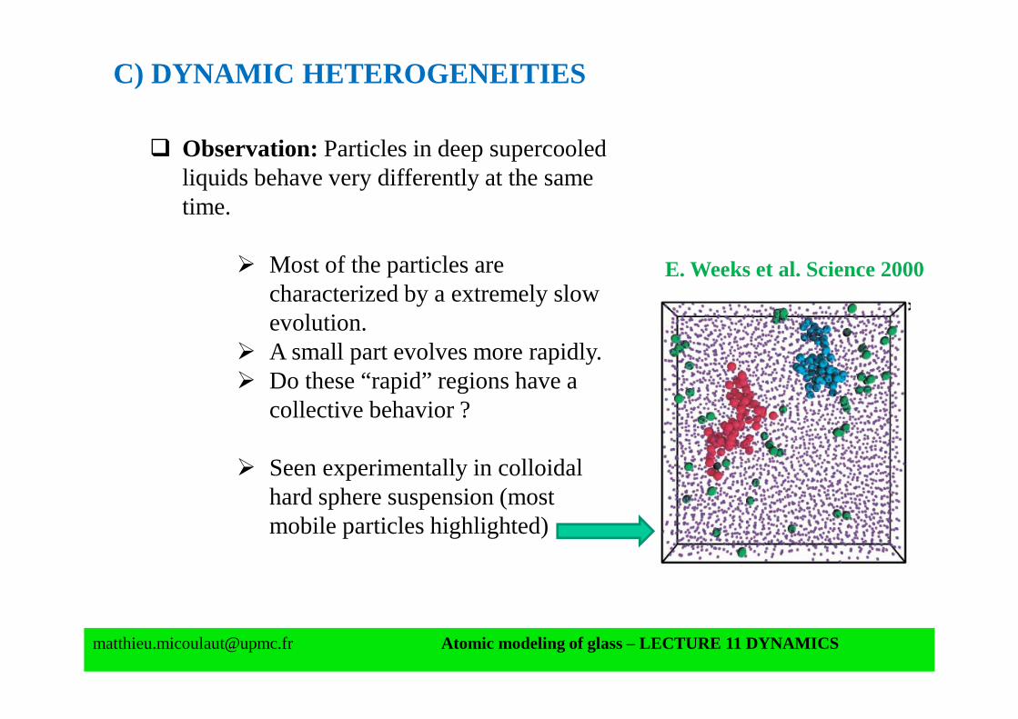
E. Weeks et al. Science 2000
Observation: Particles in deep supercooledliquids behave very differently at the same time.
Most of the particles are characterized by a extremely slow evolution.
A small part evolves more rapidly. Do these “rapid” regions have a
collective behavior ?
Seen experimentally in colloidalhard sphere suspension (mostmobile particles highlighted)
[email protected] Atomic modeling of glass – LECTURE 11 DYNAMICS
[email protected] Atomic modeling of glass – LECTURE 11 DYNAMICS
C) DYNAMIC HETEROGENEITIES
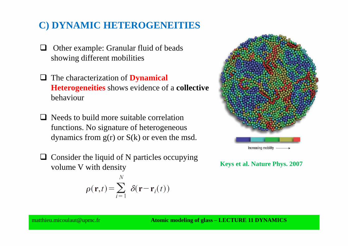
Other example: Granular fluid of beads showing different mobilities
The characterization of Dynamical Heterogeneitiesshows evidence of a collective behaviour
Needs to build more suitable correlation functions. No signature of heterogeneous dynamics from g(r) or S(k) or even the msd.
Consider the liquid of N particles occupying volume V with density Keys et al. Nature Phys. 2007
[email protected] Atomic modeling of glass – LECTURE 11 DYNAMICS
C) DYNAMIC HETEROGENEITIES
Measure of the number of ‘‘overlapping’’ particles in two configurations separated by a time interval t (time-dependent order parameter ):
out of which can be defined a fluctuation (time-dependent order parameter χ4(t):
which expresses with a four-point time-dependent density correlation function G4(r1,r2,r3,r4,t):

[email protected] Atomic modeling of glass – LECTURE 11 DYNAMICS
C) DYNAMIC HETEROGENEITIES
Four-point time dependent density correlation :
which can be reduced (isotropic media) to a function G4(r,t).
Meaning of GGGG4(r,t): Measures correlations of motion between 0 and t arising at two points, 0 and r.
Meaning of the dynamic susceptibility χχχχ4(t): Typical number of particles involved in correlated motion (volume of the correlated clusters)
[email protected] Atomic modeling of glass – LECTURE 11 DYNAMICS
C) DYNAMIC HETEROGENEITIES
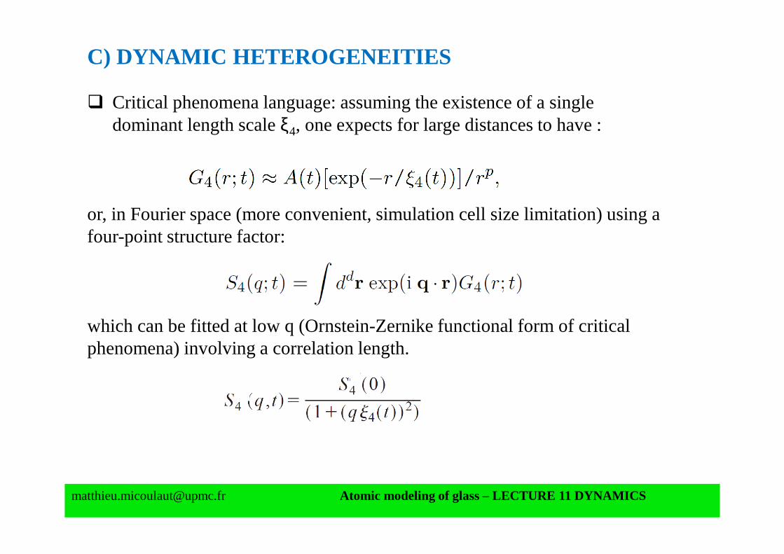
Critical phenomena language: assuming the existence of a single dominant length scale ξ4, one expects for large distances to have :
or, in Fourier space (more convenient, simulation cell size limitation) using a four-point structure factor:
which can be fitted at low q (Ornstein-Zernike functional form of critical phenomena) involving a correlation length.

[email protected] Atomic modeling of glass – LECTURE 11 DYNAMICS
C) DYNAMIC HETEROGENEITIES
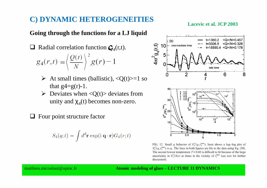
Going through the functions for a LJ liquid
Overlap order parameter Q(t)
Two-step relaxation (transient caging) similar to the behavior of the intermediate scattering function F(k,t). Decays to Qinf, random overlap, fraction of the volume occupied by particles at any given time.
Sample to sample fluctuation:
Growth of correlated motion between pairs of particles. At long times, diffusion thus χ4(t)=0.
Lacevic et al. JCP 2003
[email protected] Atomic modeling of glass – LECTURE 11 DYNAMICS
C) DYNAMIC HETEROGENEITIES
Going through the functions for a LJ liquid
Radial correlation function G4(r,t).
At small times (ballistic), <Q(t)>=1 so that g4=g(r)-1.
Deviates when <Q(t)> deviates from unity and χ4(t) becomes non-zero.
Four point structure factor
Lacevic et al. JCP 2003

[email protected] Atomic modeling of glass – LECTURE 11 DYNAMICS
C) DYNAMIC HETEROGENEITIES
Going through the functions for a LJ liquid
Fitting using the Ornstein-Zernike theory
Allows determining correlation length ξ4(t) as a function of temperature.
Correlation length ξ4(t)
Qualitatively similar to χ4(t) Increase of ξ4(t) as T decreases.
Lacevic et al. JCP 2003

[email protected] Atomic modeling of glass – LECTURE 11 DYNAMICS
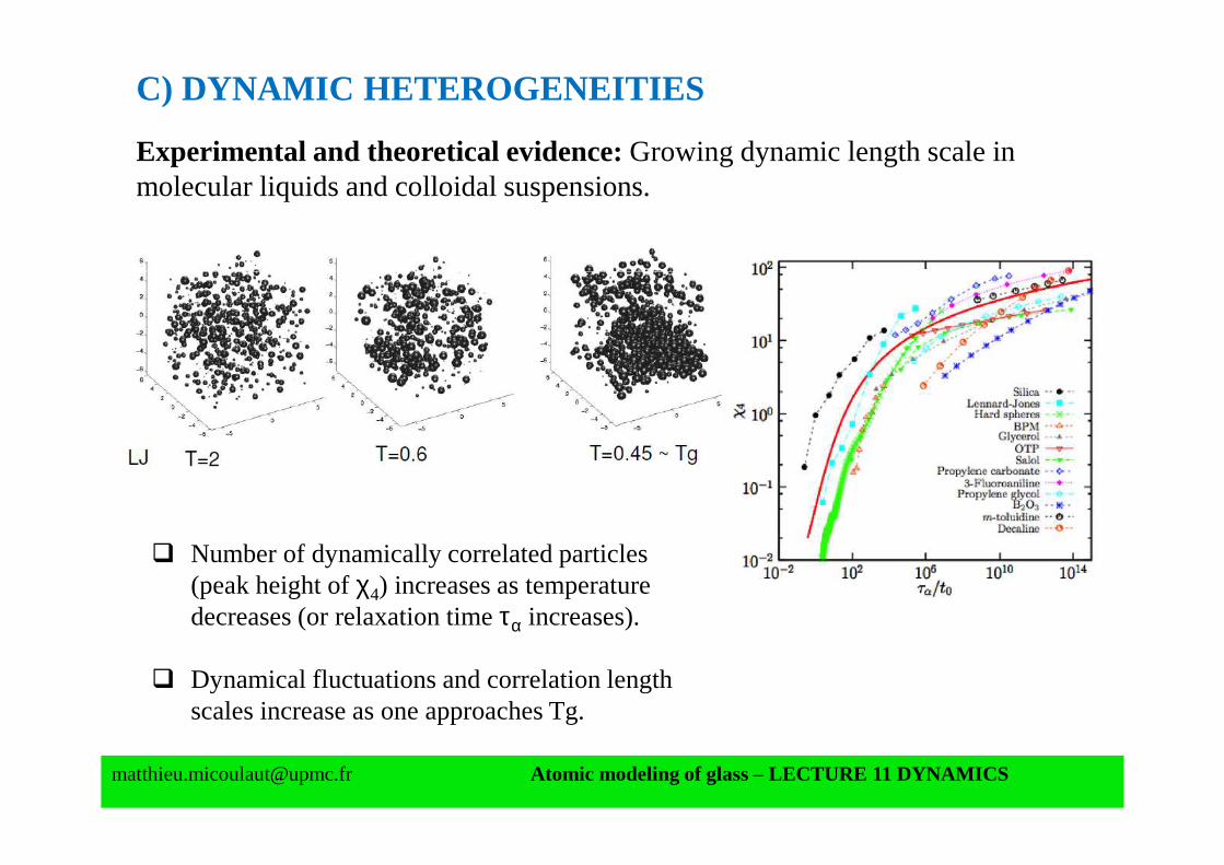
C) DYNAMIC HETEROGENEITIES
Experimental and theoretical evidence:Growing dynamic length scale in molecular liquids and colloidal suspensions.
Berthier et al. Science 2005
[email protected] Atomic modeling of glass – LECTURE 11 DYNAMICS
C) DYNAMIC HETEROGENEITIES
Experimental and theoretical evidence:Growing dynamic length scale in molecular liquids and colloidal suspensions.
Number of dynamically correlated particles(peak height of χ4) increases as temperature decreases (or relaxation time τα increases).
Dynamical fluctuations and correlation lengthscales increase as one approaches Tg.

[email protected] Atomic modeling of glass – LECTURE 11 DYNAMICS
D) ISOCONFIGURATIONAL ENSEMBLE
A. Widmer-Cooper, P. Harrowell, PRL 2004, Bertier and Lack, PRE 2007
Idea: Study of the role of local structure when approaching the glass transition. As T is lowered, it becomes harder to sample all the phase space.
Initial positions of particles are held fixed, but N dynamical trajectoriesare independent through the use of random initial velocities. N MD runs
Define Ci(t) a general dynamic object attached to particle isuch as:
Isoconfigurational average
Equilibrium Ensemble averages
Dynamic propensity e.g. displacement
[email protected] Atomic modeling of glass – LECTURE 11 DYNAMICS
D) ISOCONFIGURATIONAL ENSEMBLE
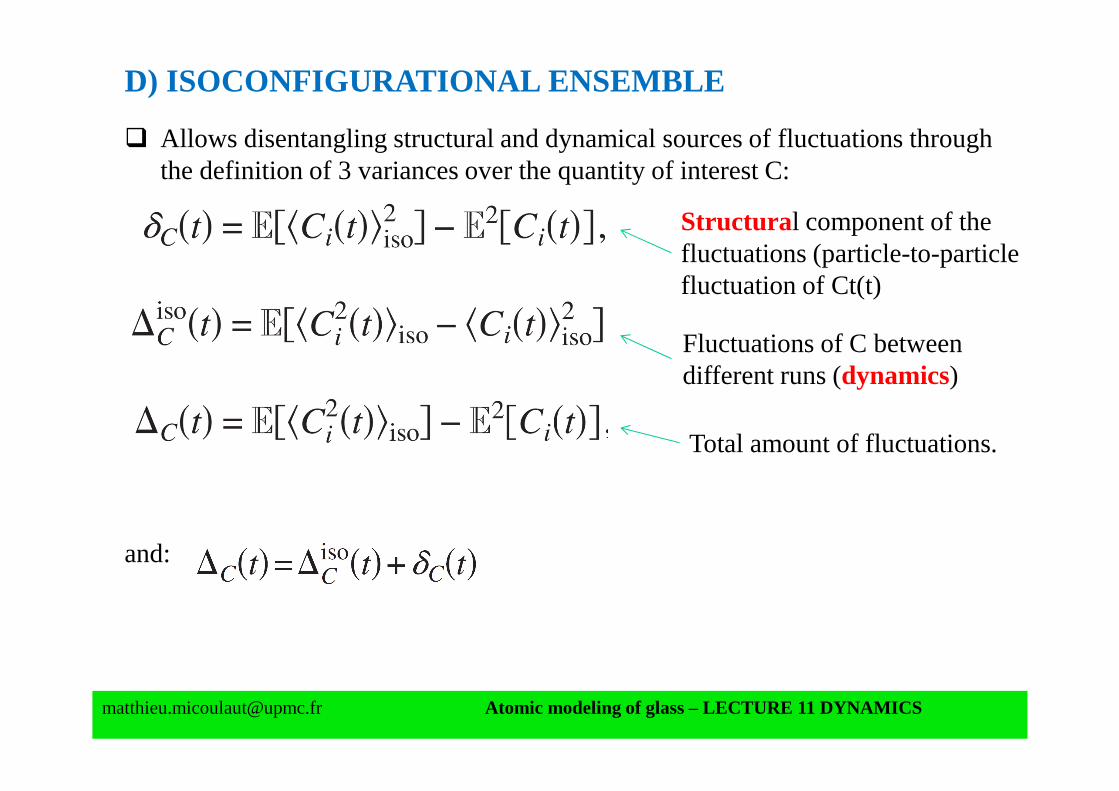
Allows disentangling structural and dynamical sources of fluctuations through the definition of 3 variances over the quantity of interest C:
and:
Fluctuations of C betweendifferent runs (dynamics)
Structura l component of the fluctuations (particle-to-particlefluctuation of Ct(t)
Total amount of fluctuations.
[email protected] Atomic modeling of glass – LECTURE 11 DYNAMICS
D) ISOCONFIGURATIONAL ENSEMBLE
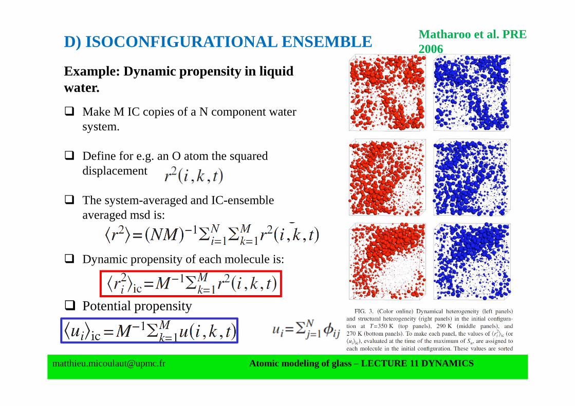
Example: Dynamic propensity in liquid water.
Make M IC copies of a N component water system.
Define for e.g. an O atom the squared displacement
The system-averaged and IC-ensemble averaged msd is:
Dynamic propensity of each molecule is:
Potential propensity
Matharoo et al. PRE 2006

[email protected] Atomic modeling of glass – LECTURE 11 DYNAMICS
D) ISOCONFIGURATIONAL ENSEMBLE
Razul et al., JPCM (2011).
Lennard-Jones liquid
[email protected] Atomic modeling of glass – LECTURE 11 DYNAMICS
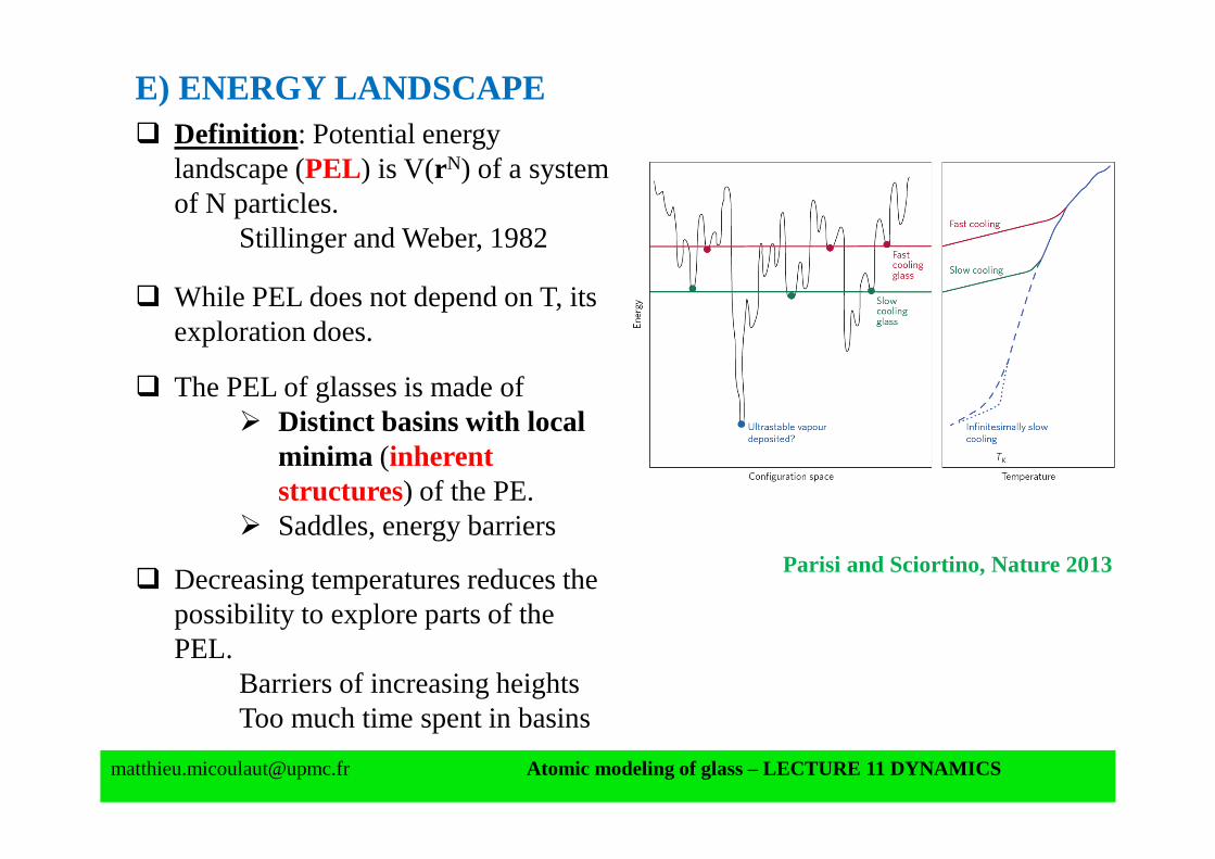
E) ENERGY LANDSCAPE Definition : Potential energy
landscape (PEL) is V(rN) of a system of N particles.
Stillinger and Weber, 1982
While PEL does not depend on T, its exploration does.
The PEL of glasses is made of Distinct basins with local
minima (inherent structures) of the PE.
Saddles, energy barriers
Decreasing temperatures reduces the possibility to explore parts of the PEL.
Barriers of increasing heightsToo much time spent in basins
Parisi and Sciortino, Nature 2013
[email protected] Atomic modeling of glass – LECTURE 11 DYNAMICS
E) ENERGY LANDSCAPE
The partition functionZ of a system of N particles interacting via a two-body spherical potential is :
Configuration space can be partitioned into basins. Partition function becomes a sum over the partition functions of the individual distinct basins Qi
Partition function averaged over all distinct basins with the sameeIS value as
and associated average basin free energy as

[email protected] Atomic modeling of glass – LECTURE 11 DYNAMICS
E) ENERGY LANDSCAPE
The partition function of the system then reduces to a sum of the IS:
Ω(eIS) is the number of basins of depth eIS.
This defines the configurationalentropy :
eIS
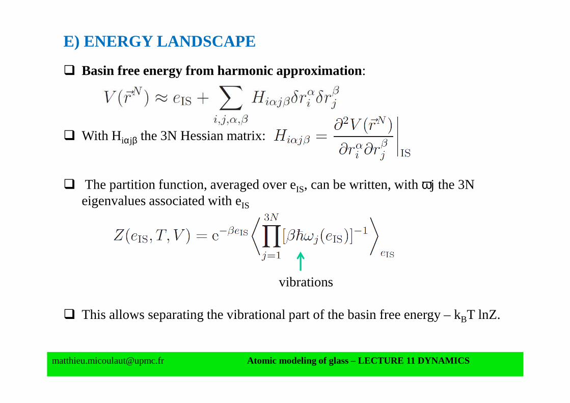
Basin free energy from harmonic approximation:
With Hiαjβ the 3N Hessian matrix:
The partition function, averaged over eIS, can be written, with ωj the 3N eigenvalues associated with eIS
vibrations
This allows separating the vibrational part of the basin free energy – kBT lnZ.
[email protected] Atomic modeling of glass – LECTURE 11 DYNAMICS
E) ENERGY LANDSCAPE
[email protected] Atomic modeling of glass – LECTURE 11 DYNAMICS
E) ENERGY LANDSCAPE
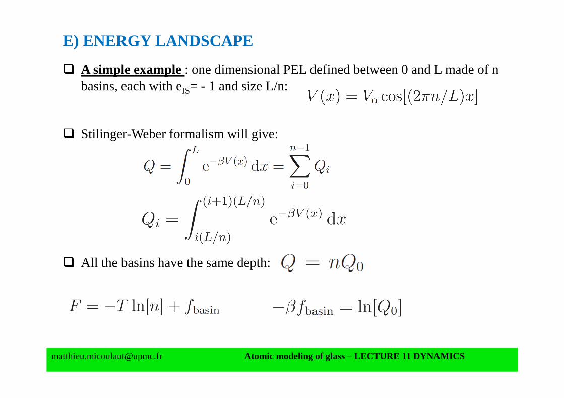
A simple example : one dimensional PEL defined between 0 and L made of n basins, each with eIS= - 1 and size L/n:
Stilinger-Weber formalism will give:
All the basins have the same depth:

[email protected] Atomic modeling of glass – LECTURE 11 DYNAMICS
E) ENERGY LANDSCAPE
BKS silica: IS energies and configurational energies
F. Sciortino, J. Stat. Mech. 2005
[email protected] Atomic modeling of glass – LECTURE 11 DYNAMICS
E) ENERGY LANDSCAPE
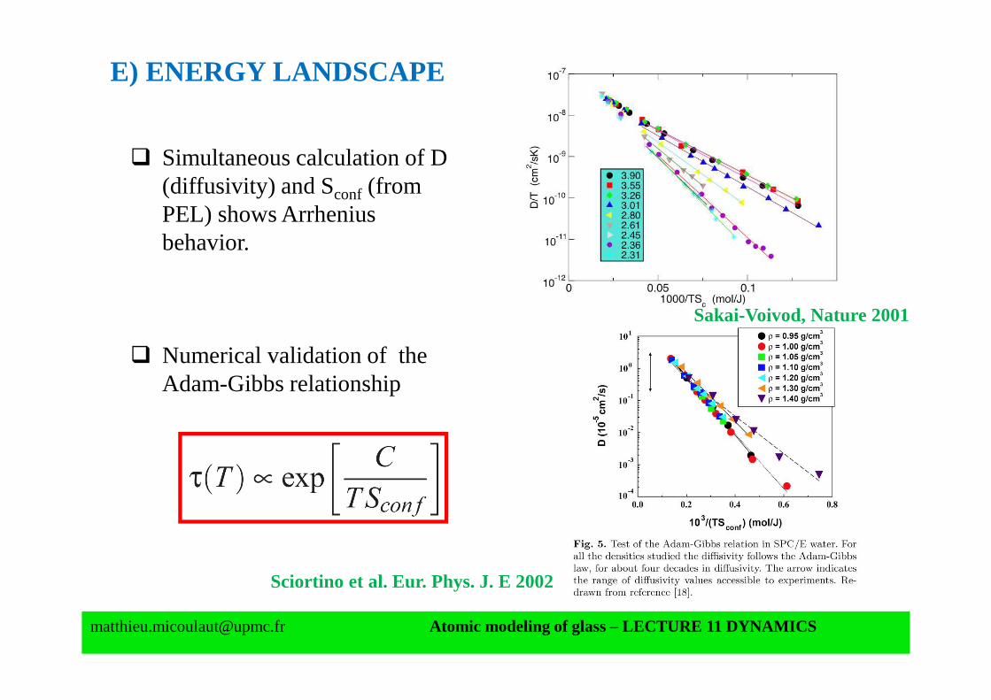
Simultaneous calculation of D (diffusivity) and Sconf (fromPEL) shows Arrhenius behavior.
Numerical validation of the Adam-Gibbs relationship
Sciortino et al. Eur. Phys. J. E 2002
Sakai-Voivod, Nature 2001
[email protected] Atomic modeling of glass – LECTURE 11 DYNAMICS
Conclusion:
Dynamics of glass-forming systems can be followed with numerous tools using computer simulations.
Functions quantify the slowing down of the dynamics.
Heterogeneous dynamics sets in: Non-Gaussian parameter, Four-point correlation functions, Isoconfigurational Ensemble
Energy landscapes provides a thermodynamic view that connects back to the simple Adam-Gibbs relationship.
Next lecture (12):Ab initio simulations…a survey