lecture 11 introduction to nonparametric regression ... – ec2 - lecture 11 1 1 lecture 11...
TRANSCRIPT
RS – EC2 - Lecture 11
1
1
Lecture 11Introduction to Nonparametric
Regression: Density Estimation
• The goal of a regression analysis is to produce a reasonable analysis to the unknown response function f, where for N data points (Xi,Yi), the relationship can be modeled as
- Note: m(.) = E[y|x] if E[ε|x]=0 –i.e., ε ┴ x
• We have different ways to model the conditional expectation function (CEF), m(.):
- Parametric approach
- Nonparametric approach
- Semi-parametric approach.
2
Non Parametric Regression: Introduction
Nixmy iii ,,1,)(
RS – EC2 - Lecture 11
2
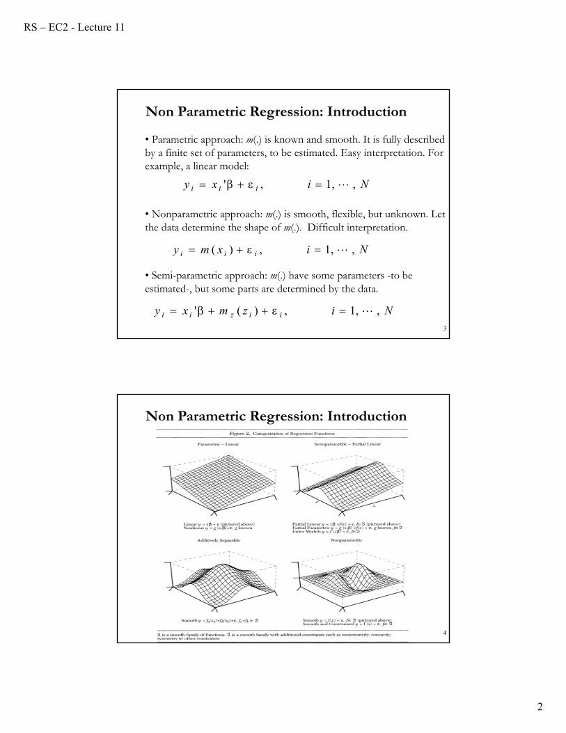
• Parametric approach: m(.) is known and smooth. It is fully described by a finite set of parameters, to be estimated. Easy interpretation. For example, a linear model:
• Nonparametric approach: m(.) is smooth, flexible, but unknown. Let the data determine the shape of m(.). Difficult interpretation.
• Semi-parametric approach: m(.) have some parameters -to be estimated-, but some parts are determined by the data.
3
Non Parametric Regression: Introduction
Nixy iii ,,1,'
Nixmy iii ,,1,)(
Nizmxy iizii ,,1,)('
4
Non Parametric Regression: Introduction
RS – EC2 - Lecture 11
3
• Parametric and non-parametric approaches use a weighted sum of the y‘s to obtain the fitted values, ŷ. That is,
ŷi = Σi ωi yi
• Instead of using equal weights as in OLS or weights proportional
to the inverse of variance as often in GLS, a different rationale determines the choice of weights in nonparametric regression.
• In the single regressor case, the observations with the most information about f(x0) should be those at locations xi closest to x0.
• Thus, a decreasing function of the distances of their locations xi
from x0 determine the weights assigned to yi’s. 5
Non Parametric Regression: Introduction
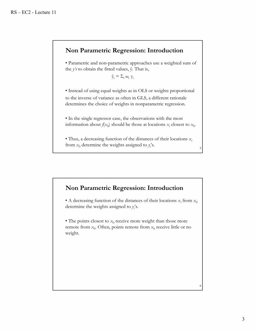
• A decreasing function of the distances of their locations xi from x0
determine the weights assigned to yi’s.
• The points closest to x0 receive more weight than those more remote from x0. Often, points remote from x0 receive little or no weight.
6
Non Parametric Regression: Introduction

RS – EC2 - Lecture 11
4
• We have a large number of observations on a RV X. We would like to “draw” the pdf of X.
• Simplest method: Use a histogram. That is, divide the range of X into a small number of intervals (bins), h, and count the number of times X, ni, is observed in each interval:
• Q: How wide should the bins be? Too small (too many bins) distribution looks jerky, too large (few bins), shape is not easy to visualize.
• Two questions: - Do we want the same bin-width everywhere?
- Do we believe the density is zero for empty bins? 7
Density Estimation: Univariate Case
N
hnp ii
)(
8
Density Estimation – Bins: Example
Changes in SF Home Prices - 50 bins
Changes in Prices
Fre
quency
-4 -2 0 2 4
05
10
15
20
25
• We use two histograms to fit percentage changes in monthly San Francisco home prices (r_sf, with N=359), with two h (large h, 10 bins; small h, 50 bins). =>Smaller h, more resolution.

RS – EC2 - Lecture 11
5
• The histogram is close to, but not truly density estimation. It does not estimate f(x) at every x. Rather, it partitions the sample space into bins, and only approximate the density at the center of each bin.
• Two problems with histograms:
(1) For a given number of bins, moving their exact location (boundary points) can change the graph.
(2) The density function produced is a step function and the derivative either equals zero or is not defined (when at the cutoff point for two bins).
- This is a problem if we are trying to maximize a likelihood function that is defined in terms of the densities of the distributions.
9
Density Estimation: Problems with Histograms
• First, define the density function for a variable x. For a particular value of x, call it x0, the density function is:
• For a sample of data on X of size N, a histogram with a column width of 2h, centering the column around x0 can be approximated by:
• This function equals the fraction of the sample that lies within h of x0, divided by the column width (2h).We call this the naive estimator.
• x0 is any value of X, not necessarily equal to any xi’s in the sample. 10
Density Estimation: Definition of Histogram
h
hxxhxob
h
hxFhxFxf hh 2
][Prlim
2
)()(lim)( 00
000
00
)1||
(1
2
])[1)(ˆ
1
0
1
000
N
i
iN
i
iHist h
xxI
Nhh
hxxhxI
Nxf
RS – EC2 - Lecture 11
6
• Dealing with the two problems:
(1) Arbitrary location of the bin cutoff points
Solution: Define a “moving” bin that is defined for every possible value of x. Then, count how many actual xi’s are within h/2 of the hypothetical point, and “normalizes” this count by the number of total observations (N) and the “bandwidth,” h.
(2) Discontinuity in the function.
Solution: Kernel density estimation (KDE). It avoids the discontinuities in the estimated (empirical) density function. In terms of histogram formula, the kernel is everything to the right of the summation sign. The general formula for the kernel estimator (Parzen window):
11
Density Estimation: Problems Revisited
)(1
)(ˆ1
00
N
i
iHist h
xxK
Nhxf
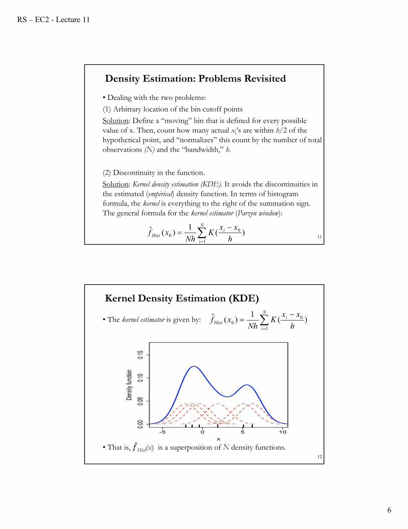
• The kernel estimator is given by:
• That is, Hist(x) is a superposition of N density functions.12
Kernel Density Estimation (KDE)
)(1
)(ˆ1
00
N
i
iHist h
xxK
Nhxf
RS – EC2 - Lecture 11
7
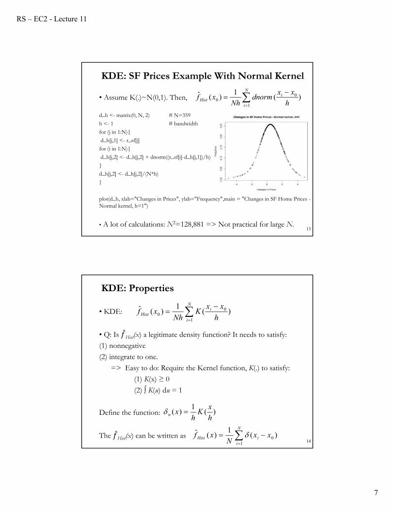
• Assume K(.)~N(0,1). Then,
d_h <- matrix(0, N, 2) # N=359
h <- 1 # bandwidth
for (j in 1:N){
d_h[j,1] <- r_sf[j]
for (i in 1:N){
d_h[j,2] <- d_h[j,2] + dnorm((r_sf[i]-d_h[j,1])/h)
}
d_h[j,2] <- d_h[j,2]/(N*h)
}
plot(d_h, xlab="Changes in Prices", ylab="Frequency",main = "Changes in SF Home Prices -Normal kernel, h=1")
• A lot of calculations: N2=128,881 => Not practical for large N.13
KDE: SF Prices Example With Normal Kernel
)(1
)(ˆ1
00
N
i
iHist h
xxdnorm
Nhxf
• KDE:
• Q: Is Hist(x) a legitimate density function? It needs to satisfy:
(1) nonnegative
(2) integrate to one.
=> Easy to do: Require the Kernel function, K(.) to satisfy:
(1) K(x) ≥ 0
(2) ∫ K(u) du = 1
Define the function:
The Hist(x) can be written as14
KDE: Properties
)(1
)(h
xK
hxn
N
iiHist xx
Nxf
10 )(
1)(ˆ
)(1
)(ˆ1
00
N
i
iHist h
xxK
Nhxf

RS – EC2 - Lecture 11
8
• Check the properties of Hist(x) and δn(x):
• The kernel function can be generalized.
Note: Any density function satisfies our requirements. For example, K(.) can be a normal density.
15
KDE: Properties
1)(1
)(1
)(ˆ
1)(1
)(
iin
iinHist
iin
dxxxN
dxxxN
xf
duuKdxh
xxK
hdxxx
• The kernel function K(.) is a continuous and bounded (usually symmetric around zero) real function which integrates to 1.
• h is a smoothing parameter (bandwidth). 2h is called the window width.
• The order of a kernel, v, is defined as the order of the first non-zero moment, κk. For example, if κ1(K) = 0 and κ 2(K) > 0 then K is a 2nd
order kernel. The order of a symmetric kernel is always even.
• Symmetric non-negative kernels are second-order kernels. We will emphasize these kernels (v=2).
• Higher-order kernels are obtained by multiplying a second-order kernel by an (2v-1)-th order polynomial in z2. See Hansen (2009).
KDE: Kernels
RS – EC2 - Lecture 11
9
• Most common kernel functions (2nd order):
- Uniform kernel: K(z) = 0.5 for |z| ≤ 1
= 0 for |z| > 1
- Epanechnikov kernel: K(z) = 0.75(1-z2) for |z| ≤ 1
= 0 for |z| > 1
- Quartic (biweight) kernel: K(z) = 15/16 (1-z2)2 for |z| ≤ 1
= 0 for |z| > 1
- Triweight kernel: K(z) = 35/32 (1-z2)3 for |z| ≤ 1
= 0 for |z| > 1
- Gaussian (normal) kernel: K(z) =1/sqrt(2π) exp(-z2/2)
• Density graph: Plot Hist(x) against x0 and connect points.
KDE: Kernels
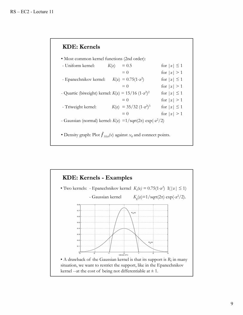
• Two kernels: - Epanechnikov kernel Ke(z) = 0.75(1-z2) I(|z| ≤ 1)
- Gaussian kernel Kg(z)=1/sqrt(2π) exp(-z2/2).
KDE: Kernels - Examples
• A drawback of the Gaussian kernel is that its support is R; in many situation, we want to restrict the support, like in the Epanechnikov kernel --at the cost of being not differentiable at ± 1.
RS – EC2 - Lecture 11
10
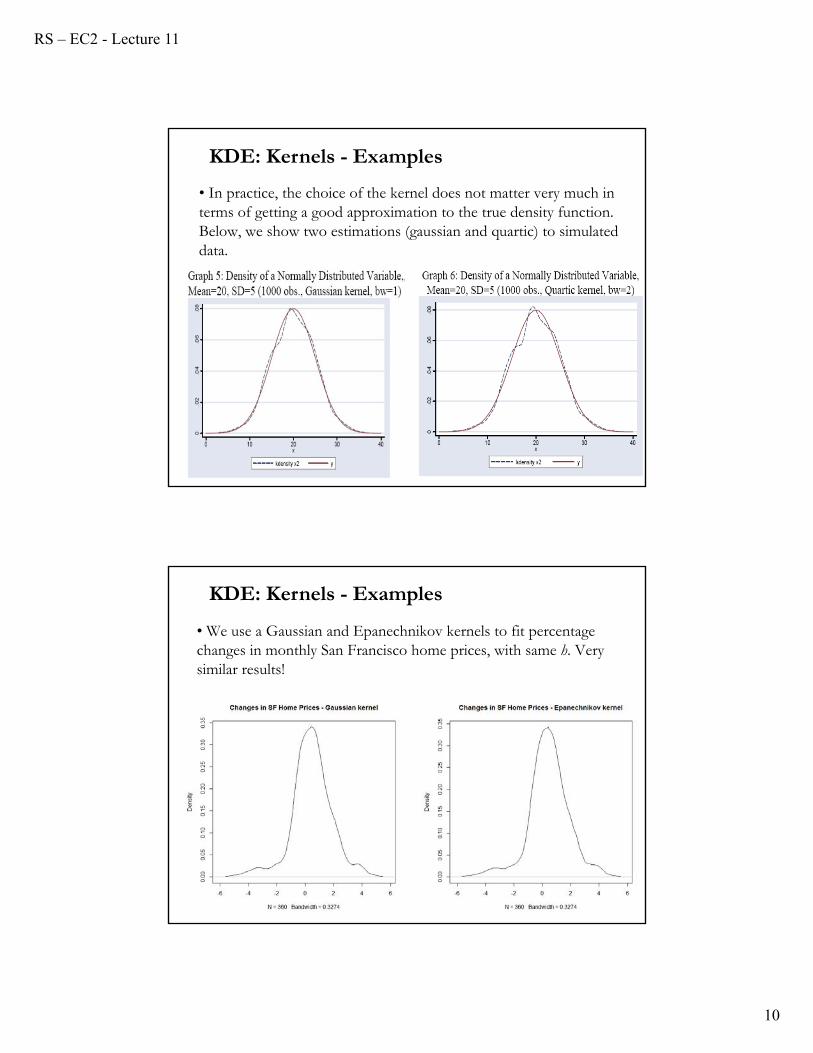
• In practice, the choice of the kernel does not matter very much in terms of getting a good approximation to the true density function. Below, we show two estimations (gaussian and quartic) to simulated data.
KDE: Kernels - Examples
• We use a Gaussian and Epanechnikov kernels to fit percentage changes in monthly San Francisco home prices, with same h. Very similar results!
KDE: Kernels - Examples

RS – EC2 - Lecture 11
11
• Expectation
where we use a change of variables u = (xi – x0)/h. We approximate the integral using a Taylor expansion of f(x0+hu) in hu (as h ⟶0):
Then, for a v-th order K(.) (then, κj=0, for j<v):
KDE: Statistical Inference
duhuxfuKduufuKN
h
xxKE
NhxfE
N
i
N
i
i
)()()()(1
)]([1
)](ˆ[
01
1
00
)()(!
1...)(''
2
1)(')()( 0
220000
vvvv houhxfv
uhxfhuxfxfhuxf
)()(!
1)(
...)(''2
1)(')()()(
00
22
01000
vv
vv hohxfv
xf
hxfhxfxfhuxfuK
• Then, the expectation is:
It is a biased! The bias depends on h, the curvature of f(.), and K(.).
• For a 2nd-order kernel, the bias is:
Note: When higher-order kernels are used, the bias is portional to hv; which is of lower order than h2. Then, higher-order kernels are
bias-reducing kernels.
KDE: Statistical Inference
)()(!
1)()](ˆ[ 000
vv
vv hohxfv
xfxfE
)()(2
1)()](ˆ[ 2
22
02
00 hohxfxfxfE

RS – EC2 - Lecture 11
12
• Variance
- From the analysis of bias we know the 2nd term is O(1/N). Recall,
E[ (x0)] = f(x0) +o(1)
- For the 1st term, we make a change of variables and use a 1st-order Taylor expansion:
KDE: Statistical Inference
20202
02
1
020
)])([1
(1
])([1
)]([1
)]([)(
1)](ˆ[
h
xxKE
hNh
xxKE
Nh
h
xxKVar
Nhh
xxKVar
NhxfVar
ii
iN
i
i
)()()(
))(()()()(])([1
0
02
0220
hOKRxf
duhOxfuKduhuxfuKh
xxKE
hi
• Then, the variance is:
⟹ The variance depends on the N, h, f(.) and K(.). It will go to 0 as Nh → ∞.
Note: We can combine the previous results (bias and variance) to measure precision of (x0) as the MSE:
which is called Asymptotic MSE (AMSE). It depends on N, h, f(.) and K(.). The bias is increasing in h, the variance decreasing in Nh.
KDE: Statistical Inference
)1
()()(
)](ˆ[ 00 N
ONh
KRxfxfVar
Nh
KRxfhxf
v
VarianceBiasxfMSE
vvv )()())((
)!(
)(
)()](ˆ[
02202
2
20

RS – EC2 - Lecture 11
13
• Consistency
For an i.i.d. sample of the RV X, for any value x0 and a fixed h, (x0) is a biased estimate of f(x0). Yet the bias goes to zero if h → 0 as N → ∞.
• For a 2nd-order K(.) the bias is given by:
⟹ The “size” of this bias is O(h2).
• Assuming that h → 0 as N → ∞, the variance of (x0) is:
Var[ (x0)] = [1/(Nh)] f(x0) ∫(K(z))2dz + o(1/Nh)
⟹ The variance will go to 0 as Nh → ∞, so h must converge to 0 at a slower rate than N goes to ∞.
KDE: Statistical Inference
duuKuxfhxfxfExfbias )()(''
2
1)()](ˆ[))(ˆ( 2
02
000
• The previous results are approximations. They were derived by approximating integrals by a Taylor expansion of f(x+hu) in the argument hu→0.
• The kernel estimator (x0) is pointwise consistent at any point x0 if both the variance and bias disappear as N → ∞ (check AMSE formula),
which requires that h → 0 and Nh → ∞.
• The uniform convergence (stronger) property holds if Nh/ln(h) → ∞.
• See Cameron and Trivedi’s (CT) textbook for formal details.
KDE: Statistical Inference

RS – EC2 - Lecture 11
14
• Asymptotic normality
The kernel estimator is the sample average. A CLT can be applied. Using previous results:
- Given the order of the variance, the rate of convergence is sqrt(Nh), not sqrt(N) as in standard regression estimates.
- The estimator is biased, so we center fˆ(x0) around its expectation.
That is, by the CLT we get:
sqrt(Nh) ( (x0)- E[ (x0)])→d N(0, f(x0 )∫(K(z))2dz)
Note: Given the bias, [ (x0)- E[ (x0)]], is also asymptotically normally distributed, but with a non-zero mean.
KDE: Statistical Inference
• As the previous formulas show, there is a genuine trade-off between avoiding bias and reducing the variance of the estimate at any given point x.
• In general, large h reduce the variance by smoothing over a large number of points, but this is likely to lead to bias because the points are “averaged” in a mechanical way that does not account for the particular shape of the distribution.
• In contrast, small h give higher variance but have less bias. In the limit, h→0, the kernel reproduced the data.
• We can play with different h’s, but we would like a data-driven bandwidth (“automatic”) selection process.
KDE: Bandwidth

RS – EC2 - Lecture 11
15
KDE: Bandwidth - Examples
KDE: Bandwidth - Examples
RS – EC2 - Lecture 11
16
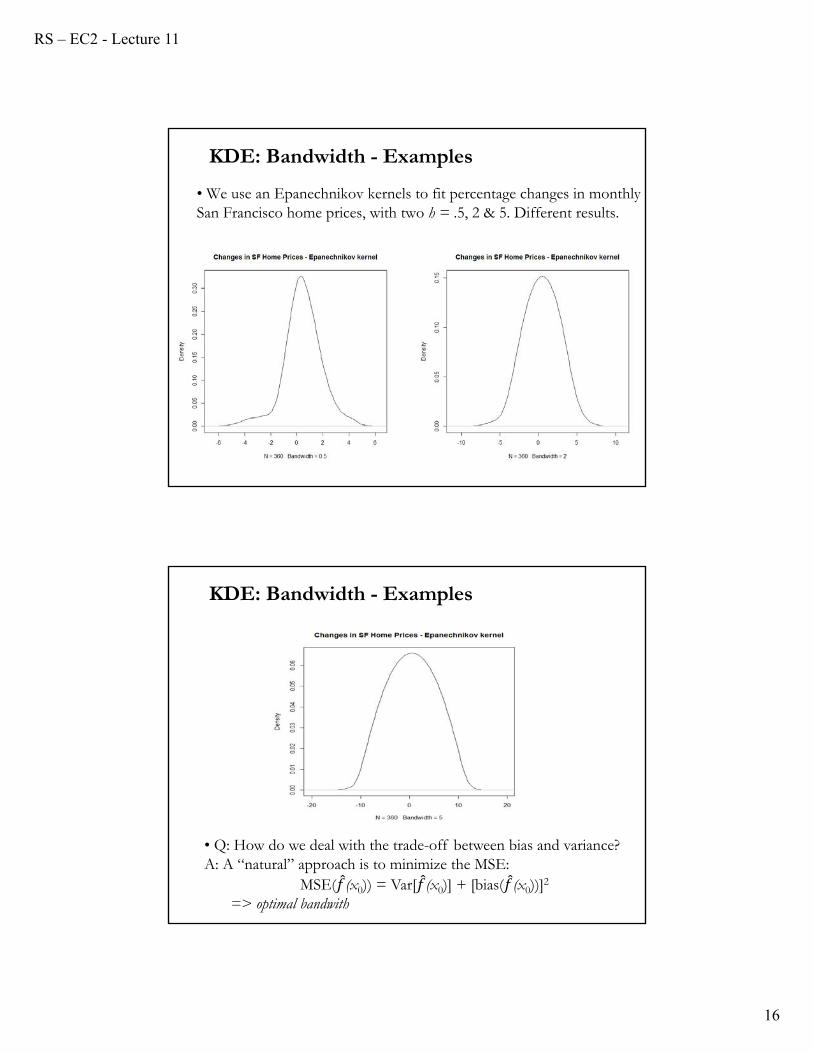
KDE: Bandwidth - Examples
• We use an Epanechnikov kernels to fit percentage changes in monthly San Francisco home prices, with two h = .5, 2 & 5. Different results.
KDE: Bandwidth - Examples
• Q: How do we deal with the trade-off between bias and variance? A: A “natural” approach is to minimize the MSE:
MSE( (x0)) = Var[ (x0)] + [bias( (x0))]2
=> optimal bandwith

RS – EC2 - Lecture 11
17
KDE: Bandwidth - Selection
• A “natural” approach is to minimize the MSE:MSE( (x0)) = Var[ (x0)] + [bias( (x0))]2
• As shown in previous formulas, the bias is O(h2) and the variance isO(1/Nh). Intuitively, h should be chosen to that the (bias)2 and the variance are of the same order.
• The square of the bias is O(h4) => h4 = 1/Nh, => h = (1/N)1/5.
That is, h = O(N-0.2) and sqrt(Nh) = O(N 0.4).
• A more formal derivation is given on C&T.
• Note: Recall that the MSE is approximated using asymptotic expansion. We called it AMSE (asymptotic MSE).
KDE: Bandwith and MISE
• Rosenblatt (1956) developed a global measure of accuracy for (x0): Minimizing the SSE at a large number of hypothetical points. As this number goes to infinity, this amounts to minimizing the mean of the integrated squared error (MISE). If the previous asymptotic approximations are used, the MISE becomes AMISE.
• That is, an optimal bandwidth minimizes MISE(h) = E[ ∫( (x0)-f(x0))2 dx0] = E[ ∫ MSE( (x0)) dx0]
• Differentiating AMISE(h) w.r.t. h yields the optimal bandwidth:h* = δ [∫ (f’’(x0)2 dx0 ]-0.2 N-0.2,
where δ depends on the kernel function used:δ = [∫ (K(z))2 dz]0.2 [∫ z2 K(z) dz]-0.4.
• Note: ∫ (K(z))2 dz is called the roughness of K(.).

RS – EC2 - Lecture 11
18
KDE: Optimal Bandwith
• The optimal bandwidth, h*:h* = δ [∫ (f ′′(x0)2 dx0 ]-0.2 N-0.2.
• The optimal bandwidth decreases (very slowly) as N increases. Then, h* → 0 as N → ∞ (as required for consistency).
• h* depends on δ, which is a function of the kernel K( ). For example, if K(.) is Gaussian,
δ = [∫ (K(z))2 dz]0.2 [∫ z2 K(z) dz]-0.4 = [1/(2*sqrt(π))]0.2 [σ2=1]-0.4
= [1/(2*sqrt(π))]0.2 (=.776388)
• Values for δ are given in Table 9.1 in C&T.
• This result also shows that if the true density function has a lot of curvature (f ′′(x) is large), the bandwidth should be smaller.
KDE: Optimality
• The optimal h* is unknown –we do not know f(x0) or f ′′(x0). Approximations methods are required.
• In practice, a normal density is commonly used instead of f(x0). Silverman’s (1986) rule of thumb assumes f ~ N(μ,σ2), then:
h* (4σ5/3N) 0.2 1.059 σ N-0.2
• As seen in the graphs, the choice of the kernel matters very little. More formally, MISE(h*) varies little across the different kernels.
• Technically speaking we can select the best kernel. The one that minimizes the AMISE. It is a calculus of variation problem
• The Epanechnikov (1969) kernel is “optimal,” but the advantage is small. It is often used to judge the efficiency of a kernel.
RS – EC2 - Lecture 11
19
KDE: Confidence Intervals
• We can obtain confidence intervals for estimates of f(x0) for any point x0. Use the variance formula above to get the conventional C.I.:
f(x0) ∈ (x0) – bias(x0) ± zα/2 sqrt{(1/Nh) (x0) [∫ (K(z))2 dz]}
where bias(x0) is given above and we have assumed that (x0) is asymptotically normal.
• Problem: It can contain negative values. Solution: Consider constructing the C.I. by inverting a test statistic.
C(x) = {f: | (x0) –bias(x0)|/[sqrt{(1/Nh) (x0) ∫ (K(z))2 dz]}≤ zα/2}
This set must be found numerically.
• In practice, it is hard to calculate the bias, and, there may not be a reason to calculate the C.I. for (x0).
KDE in Practice: Bandwidth Selection
• As mentioned above to calculate h* we need the unknown f ′′(x0). Approximations methods are required. In practice, a normal density is commonly used instead of f(x0).
1. If X ~Normal, then we get [∫ (f ′′(x0)2 dx0 ]-0.2 = 1.3643h* = δ [∫ (f ′′(x0)2 dx0 ]-0.2 N-0.2 = 1.3643 δ N-0.2 σ, σ =SD(x).
If in addition, K(.) is normal (δ=.776388) => h* = 1.059 N-0.2 σ.If in addition, K(.) is the Epanechnikov => h* = 2.34 N-0.2 σ.
2. A refinement of the formula in (1), to account for outliers, is h* = 1.3643 δ N-0.2 min[σ, iqr/1.349],
where “iqr” is the (sample) interquartile range.
• These rules for selecting h* are generally called rules of thumb.

RS – EC2 - Lecture 11
20
KDE in Practice: Boundary Effects
• So far, we have not paid much attention to the boundaries of the data, implicitly assuming that the density is supported on the entire R.
• In many situations, this is not the case. Then, the estimator can behave quite poorly due to what are called boundary effects.
• At the boundaries, (x0) usually underestimates f(x0). Suppose the data is positive, then (x0=0) penalizes x0=0 for lack of data. At x0=0,
(x0) is inconsistent.
• Many proposed techniques to deal with boundary effects:– Reflection of data (“reflect” data at x0=0, –x1, –x2 ,...,–xQ).– Transformation of data (use a function g(x); estimate (x0) instead).– Pseudo-Data Methods (“add” reasonable data, say by interpolation). – Boundary Kernel Methods (use a non-symmetric K(.) at x0=0).
• To get Hist(x) exactly, we must calculate for all x’s (x1, ..., xN):
• Then, the number of evaluations of K(.) is proportional to N2 (for a bounded Kernel, like the Epanechnikov, we have h N2 evaluations). This increases the computation time if the N is large.
• For graphing the density, we do not need to evaluate K(.) at all x’s. Instead, Hist(x) can be computed at using some points, for example using an equidistant grid z1, z2, ..., zM:
zk = xmin + (k/M) (xmax – xmin), k = 1, 2, ...., M << N
• Now, we only need M*h*N K(.) evaluations. But, we can do better by “binning” the data –i.e., using a “binned estimator.”
KDE in Practice: Computational Issues
Njh
xxK
Nhxf
N
i
jijHist ,...,1),(
1)(ˆ
1

RS – EC2 - Lecture 11
21
• For the SF changes in home prices data, we do KDE, with M=100.
M <- 100
d_h <- matrix(0, M, 2)
h <- .5
dist <- (max(r_sf)- min(r_sf))/1
for (j in 1:M){
d_h[j,1] <- min(r_sf) + j/M*dist
for (i in 1:N){
d_h[j,2] <- d_h[j,2] + dnorm((r_sf[i] - d_h[j,1])/h)
}
d_h[j,2] <- d_h[j,2]/(N*h)
}
plot(d_h, xlab="Changes in Prices", ylab="Frequency",main = "Changes in SF Home Prices -Normal kernel, h=.5")
• Still a lot of calculations: M*N=35,900 (better than N^2 = 128,881)41
KDE in Practie: Computational Issues -
• Binning or WARPing (Weighted Average of Rounded Points) “bins” the data in bins of length d starting at the origin x1. Each xi is replaced by the bincenter of the corresponding bin.
• A usual choice for d is to use h/5 or (xmin – xmax)/100. In the latter case, the effective sample size (or number of grid points) R for the computation (the number of nonempty bins) can be at most 101.
• Now, K(.) needs to be evaluated only at l d/h, where l=1,..., s, where s is the number of bins which contains the support of K(.):
computed on the grid wj = (j+0.5) d (j integer) with Ni and Nj denoting the number of observations in the i-th and j-th bins, respectively.
KDE in Practice: Computational Issues
Rjh
djiKN
Nh
Nwf
R
i
ji
jjHist ,...,1),
)(()(ˆ
1
RS – EC2 - Lecture 11
22
• The WARPing approximation requires (h*R/d) evaluations of K(.) and N + (h*R/d) steps in total.
• Much faster than the exact computation, when N is large.
• The accuracy of binned estimators has been studied by Hall (1982), and Hall and Wand (1996), among others. The accuracy depends on the number of grid points R and can be made arbitrarily good by increasing R, at the cost of increasing the number of computations.
• Hall and Wand (1996) proposed that using R between 100 and 500 should give a reasonably good approximation.
KDE in Practice: Computational Issues
• For all but very small N, direct computation of K(.) is inefficient. By noticing that the KDE is based on a convolution of the data with the K(.), fast Fourier transformations (FFT) speed up computations:
(x) = (2 )-1/2 exp(ixt) f(t) dt (Fourier transform)
• Recall the convolution theorem:
If g(x) and k(x) are integrable functions with Fourier transforms (ξ) and (ξ) respectively, then the Fourier transform of the convolution is given by the product of the Fourier transforms (ξ) and (ξ). That is,
if f(x) = g(y) k(x-y) dy,
then, (ξ) = (ξ) (ξ). => invert (ξ) to get f(ξ)!
• Another approach: Fast Gaussian transformations (FGT).
KDE in Practice: Computational Issues

RS – EC2 - Lecture 11
23
KDE in R
• Kernel density estimates are available in R via the density function:d <- density(r_sf, kernel=c("epanechnikov"), bw = .5)plot(d, main = "Changes in SF Home Prices - Epanechnikov kernel")
which reproduces a previous density plot for SF home price changes, using the Epanechnikov kernel, with h=.5 (or bw =.5).
• By default, density uses a Gaussian kernel, but a large variety of other kernels are available by specifying the kernel option, like above with kernel=c("epanechnikov"),
• By default, density selects the bandwidth based on Silverman’s (1986) rule of thumb. Other inputs (and manual inputs) can be used.
Estimating the Derivative of a Density
• Sometimes we need to estimate f ′(x) or even f ′′(x) –like in a C.I.
• One approach for estimating f ′(x) is straightforward:f ′(x) = [ (x0+Δ) – (x0-Δ)]/2Δ,
for some small Δ.
• Alternatively, differentiate the expression with respect to x0:
• We can extend this approach to get the r-th derivative:
)(1
)(ˆ1
00
N
i
i
h
xxK
Nhxf
)('1
)('ˆ
1
020
N
i
i
h
xxK
Nhxf
)(1
)(ˆ1
0)(10
)(
N
i
irr
r
h
xxK
Nhxf

RS – EC2 - Lecture 11
24
Estimating the Derivative of a Density
• Since the Gaussian kernel has derivatives of all orders this is a common choice for derivative estimation.
• The estimator of f(r)(x) is biased –same order as for estimation of f(x). But the variance is of a much larger order.
• We can derive an optimal bandwidth, we can optimize MISE(h), as before.
• In practice, for either method, you should use a larger bandwidth than you use for estimating (x0).
• We can also ask the question of which kernel function is optimal. Muller (1984) found that the Biweight class is the optimal for the first derivative and for a second derivative the Triweight class.
• So far, h has been fixed. But, this may not be optimal: what works fine in areas of high density may not necessarily be appropriate in a low-density regions.
• A possibility is to vary h, to use adaptive bandwidth kernel estimators, in which the bandwidth changes as a function of x0.
• Idea: Where there is a lot of data, we use a small neighborhood around x0; but in areas with few data points, we expand the neighborhood. That is, hi=h(xi)
• But, note that these estimators introduce added bias in regions with little data in order to reduce variance there. The bias-variance trade-off is still there.
Density Estimation: Adaptive Kernels
RS – EC2 - Lecture 11
25
Density Estimation: k-Nearest Neighbor
• In K-Nearest Neighbor (k-NN), instead of fixing bin width h and counting the number of instances, we fix the instances (neighbors) k and check bin width.
• The neighborhood is defined through those X–variables which are among the k-nearest neighbors of x.
• The observations ranked by the distances, or “nearest neighbors,” are (x(1), ..., x(N)): The k-th nearest neighbor (or k-NN of x is x(k)):
• The k-NN estimator is given by:
where dk(x) is the ordered distance to k-th closest instance to x. dk(x)is usually the Euclidian distance (others, OK: Minkowski, Manhattan).
00, 2)(ˆ
xNd
kxf
kNNkHist
Density Estimation: k-Nearest Neighbor
• The k-NN estimator is given by:
a function of dk(x). If we use the Euclidian distance, dk(x) = ∥x - x(k)∥.
• Intuitively, we allow the bandwidth to vary depending on the density of the function. At areas of low density, we use a higher bandwidth to average over a larger number of (dispersed) points.
• While the traditional k-NN estimator uses a uniform kernel, smooth kernels can also be used. For example:
In this case, the estimator is not just a function of dk(x).
00, 2)(ˆ
xNd
kxf
kNNkHist
Njxd
xxK
xNdxf
N
i jk
ji
jkjNNk ,...,1,
)()(
1)(ˆ
1
RS – EC2 - Lecture 11
26
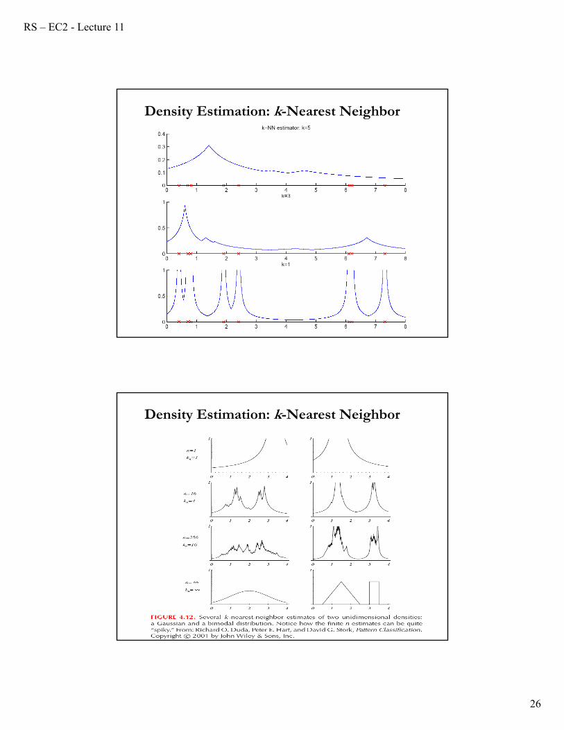
Density Estimation: k-Nearest Neighbor
Density Estimation: k-Nearest Neighbor
RS – EC2 - Lecture 11
27
Density Estimation: Observations
• k-NN density estimation has a lot of discontinuities (very spiky, not differentiable). For small N, it is not even a density!
• Even for large regions with no observed data the estimated density is far from zero (tails are too heavy).
• Same trade-off as in selecting h: A smaller k allows only nearby data points to be considered (reduce bias); but a larger k allows for smoothness (reduce variance). Not easy to balance both issues.
• Given the variance-bias trade-off, selecting k is similar to selecting h (though k is an integer). There is no clear rule of thumb or optimality rule. Some proposals exist, but practictioners insist on “know your data” to select k.
Density Estimation: Kernel or k-NN?
• The asymptotic analysis of the k-NN estimator are complicated by the fact that dk(x) is random. The solution is to condition on dk(x), which is similar to treating it as fixed.
• Then, the conditional bias and variance are identical to those of the standard kernel estimator.
• For the unconditional bias, we need moments of dk(x), under Euclidian distance, given by the k-th order statistics. It turns out that the MSE behaves similarly to the kernel estimator’s MSE.
• Q: Which one is better?
Not clear. In the tails, the Kernel estimator has smaller bias, but larger variance (the k-NN tends to be smoother in the tails).
RS – EC2 - Lecture 11
28
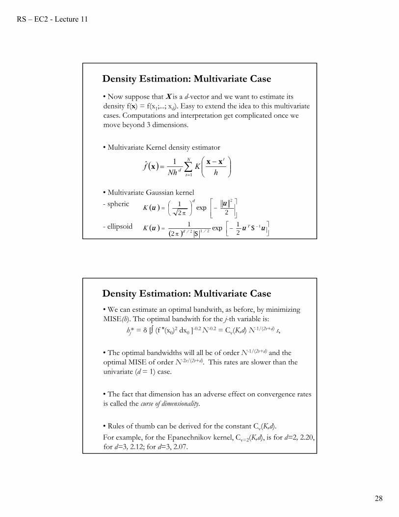
Density Estimation: Multivariate Case
• Now suppose that X is a d-vector and we want to estimate its density f(x) = f(x1;...; xd). Easy to extend the idea to this multivariate cases. Computations and interpretation get complicated once we move beyond 3 dimensions.
• Multivariate Kernel density estimator
• Multivariate Gaussian kernel
- spheric
- ellipsoid
N
t
t
d hK
Nhf
1
1ˆ xxx
uuu
uu
1212
2
21
exp2
1
2exp
2
1
SS
T//d
d
K
K
Density Estimation: Multivariate Case
• We can estimate an optimal bandwith, as before, by minimizing MISE(h). The optimal bandwith for the j-th variable is:
hj* = δ [∫ (f ′′(x0)2 dx0 ]-0.2 N-0.2 = Cv(K,d) N-1/(2v+d) s,
• The optimal bandwidths will all be of order N-1/(2v+d) and the optimal MISE of order N-2v/(2v+d). This rates are slower than the univariate (d = 1) case.
• The fact that dimension has an adverse effect on convergence rates is called the curse of dimensionality.
• Rules of thumb can be derived for the constant Cv(K,d).
For example, for the Epanechnikov kernel, Cv=2(K,d), is for d=2, 2.20, for d=3, 2.12; for d=3, 2.07.

RS – EC2 - Lecture 11
29
• Cameron, A. and P. Trivedi (2003), Microeconometrics: Methods and Applications, Cambridge University Press.
• Hardle (1990), Applied Nonparametric Regression
• Yatchew, A (2003), Semiparametic Regression for the Applied Econometrician, Cambridge University Press.
• Silverman, B. W. (1986), Density Estimation for Statistics and Data Analysis.
Readings