Lecture 12:Dense Linear Algebra

David Bindel

3 Mar 2010

HW 2 update

I I have speed-up over the (tuned) serial code!I ... provided n > 2000I ... and I don’t think I’ve seen 2×

I What I expect from youI Timing experiments with basic code!I A faster working versionI Plausible parallel versionsI ... but not necessarily great speed-up

Where we are

I Mostly done with parallel programming modelsI I’ll talk about GAS languages (UPC) laterI Someone will talk about CUDA!

I Lightning overview of parallel simulationI Recurring theme: linear algebra!I Sparse matvec and company appear often

I Today: some dense linear algebra

Numerical linear algebra in a nutshell

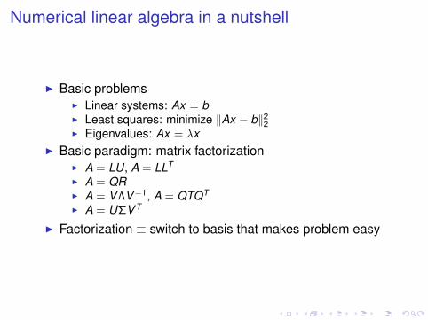
I Basic problemsI Linear systems: Ax = bI Least squares: minimize ‖Ax − b‖2

2I Eigenvalues: Ax = λx

I Basic paradigm: matrix factorizationI A = LU, A = LLT

I A = QRI A = V ΛV−1, A = QTQT

I A = UΣV T

I Factorization ≡ switch to basis that makes problem easy

Numerical linear algebra in a nutshell

Two flavors: dense and sparseI Dense == common structures, no complicated indexing

I General dense (all entries nonzero)I Banded (zero below/above some diagonal)I Symmetric/HermitianI Standard, robust algorithms (LAPACK)

I Sparse == stuff not stored in dense form!I Maybe few nonzeros (e.g. compressed sparse row formats)I May be implicit (e.g. via finite differencing)I May be “dense”, but with compact repn (e.g. via FFT)I Most algorithms are iterative; wider variety, more subtleI Build on dense ideas

History

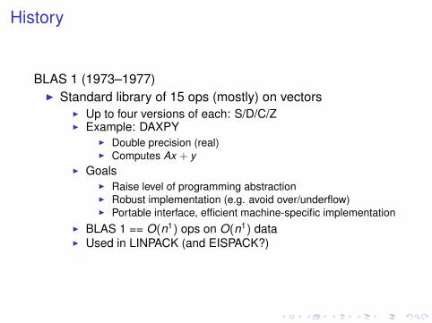
BLAS 1 (1973–1977)I Standard library of 15 ops (mostly) on vectors

I Up to four versions of each: S/D/C/ZI Example: DAXPY

I Double precision (real)I Computes Ax + y

I GoalsI Raise level of programming abstractionI Robust implementation (e.g. avoid over/underflow)I Portable interface, efficient machine-specific implementation

I BLAS 1 == O(n1) ops on O(n1) dataI Used in LINPACK (and EISPACK?)

History

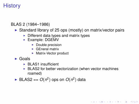
BLAS 2 (1984–1986)I Standard library of 25 ops (mostly) on matrix/vector pairs

I Different data types and matrix typesI Example: DGEMV

I Double precisionI GEneral matrixI Matrix-Vector product

I GoalsI BLAS1 insufficientI BLAS2 for better vectorization (when vector machines

roamed)I BLAS2 == O(n2) ops on O(n2) data

History

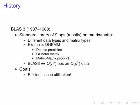
BLAS 3 (1987–1988)I Standard library of 9 ops (mostly) on matrix/matrix

I Different data types and matrix typesI Example: DGEMM

I Double precisionI GEneral matrixI Matrix-Matrix product

I BLAS3 == O(n3) ops on O(n2) dataI Goals

I Efficient cache utilization!

BLAS goes on

I http://www.netlib.org/blas

I CBLAS interface standardizedI Lots of implementations (MKL, Veclib, ATLAS, Goto, ...)I Still new developments (XBLAS, tuning for GPUs, ...)

Why BLAS?

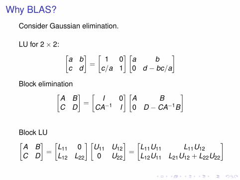
Consider Gaussian elimination.

LU for 2× 2: [a bc d

]=

[1 0

c/a 1

] [a b0 d − bc/a

]Block elimination[

A BC D

]=

[I 0

CA−1 I

] [A B0 D − CA−1B

]

Block LU[A BC D

]=

[L11 0L12 L22

] [U11 U120 U22

]=

[L11U11 L11U12L12U11 L21U12 + L22U22

]

Why BLAS?

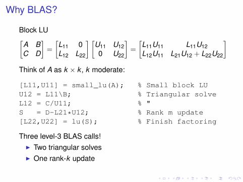
Block LU[A BC D

]=

[L11 0L12 L22

] [U11 U120 U22

]=

[L11U11 L11U12L12U11 L21U12 + L22U22

]Think of A as k × k , k moderate:

[L11,U11] = small_lu(A); % Small block LUU12 = L11\B; % Triangular solveL12 = C/U11; % "S = D-L21*U12; % Rank m update[L22,U22] = lu(S); % Finish factoring

Three level-3 BLAS calls!I Two triangular solvesI One rank-k update

LAPACK

LAPACK (1989–present):http://www.netlib.org/lapack

I Supercedes earlier LINPACK and EISPACKI High performance through BLAS

I Parallel to the extent BLAS are parallel (on SMP)I Linear systems and least squares are nearly 100% BLAS 3I Eigenproblems, SVD — only about 50% BLAS 3

I Careful error bounds on everythingI Lots of variants for different structures

ScaLAPACK

ScaLAPACK (1995–present):http://www.netlib.org/scalapack

I MPI implementationsI Only a small subset of LAPACK functionality

Why is ScaLAPACK not all of LAPACK?

Consider what LAPACK contains...

Decoding LAPACK names

I F77 =⇒ limited characters per nameI General scheme:

I Data type (double/single/double complex/single complex)I Matrix type (general/symmetric, banded/not banded)I Operation type

I Example: DGETRFI Double precisionI GEneral matrixI TRiangular Factorization

I Example: DSYEVXI Double precisionI General SYmmetric matrixI EigenValue computation, eXpert driver

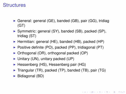
Structures

I General: general (GE), banded (GB), pair (GG), tridiag(GT)

I Symmetric: general (SY), banded (SB), packed (SP),tridiag (ST)

I Hermitian: general (HE), banded (HB), packed (HP)I Positive definite (PO), packed (PP), tridiagonal (PT)I Orthogonal (OR), orthogonal packed (OP)I Unitary (UN), unitary packed (UP)I Hessenberg (HS), Hessenberg pair (HG)I Triangular (TR), packed (TP), banded (TB), pair (TG)I Bidiagonal (BD)

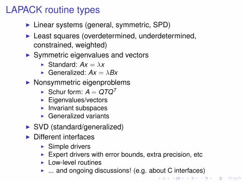
LAPACK routine typesI Linear systems (general, symmetric, SPD)I Least squares (overdetermined, underdetermined,

constrained, weighted)I Symmetric eigenvalues and vectors

I Standard: Ax = λxI Generalized: Ax = λBx

I Nonsymmetric eigenproblemsI Schur form: A = QTQT

I Eigenvalues/vectorsI Invariant subspacesI Generalized variants

I SVD (standard/generalized)I Different interfaces

I Simple driversI Expert drivers with error bounds, extra precision, etcI Low-level routinesI ... and ongoing discussions! (e.g. about C interfaces)

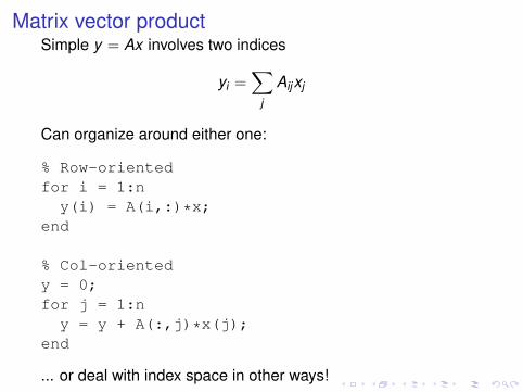
Matrix vector productSimple y = Ax involves two indices

yi =∑

j

Aijxj

Can organize around either one:

% Row-orientedfor i = 1:ny(i) = A(i,:)*x;

end

% Col-orientedy = 0;for j = 1:ny = y + A(:,j)*x(j);

end

... or deal with index space in other ways!

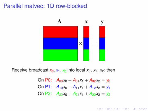
Parallel matvec: 1D row-blocked

yA x

Receive broadcast x0, x1, x2 into local x0, x1, x2; then

On P0: A00x0 + A01x1 + A02x2 = y0

On P1: A10x0 + A11x1 + A12x2 = y1

On P2: A20x0 + A21x1 + A22x2 = y2

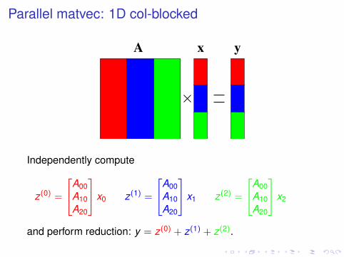
Parallel matvec: 1D col-blocked

yA x

Independently compute

z(0) =

A00A10A20

x0 z(1) =

A00A10A20

x1 z(2) =

A00A10A20

x2

and perform reduction: y = z(0) + z(1) + z(2).

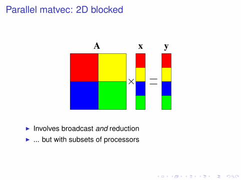
Parallel matvec: 2D blocked

yA x

I Involves broadcast and reductionI ... but with subsets of processors

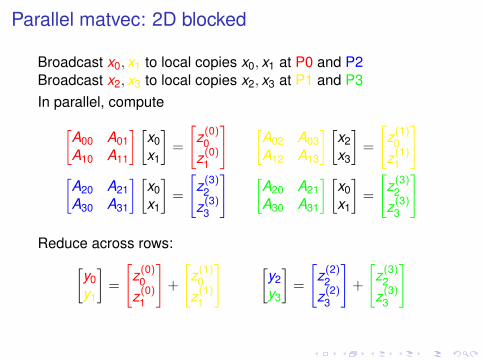
Parallel matvec: 2D blocked

Broadcast x0, x1 to local copies x0, x1 at P0 and P2Broadcast x2, x3 to local copies x2, x3 at P1 and P3In parallel, compute[

A00 A01A10 A11

] [x0x1

]=

[z(0)

0z(0)

1

] [A02 A03A12 A13

] [x2x3

]=

[z(1)

0z(1)

1

][A20 A21A30 A31

] [x0x1

]=

[z(3)

2z(3)

3

] [A20 A21A30 A31

] [x0x1

]=

[z(3)

2z(3)

3

]

Reduce across rows:[y0y1

]=

[z(0)

0z(0)

1

]+

[z(1)

0z(1)

1

] [y2y3

]=

[z(2)

2z(2)

3

]+

[z(3)

2z(3)

3

]

Parallel matmul

I Basic operation: C = C + ABI Computation: 2n3 flopsI Goal: 2n3/p flops per processor, minimal communication

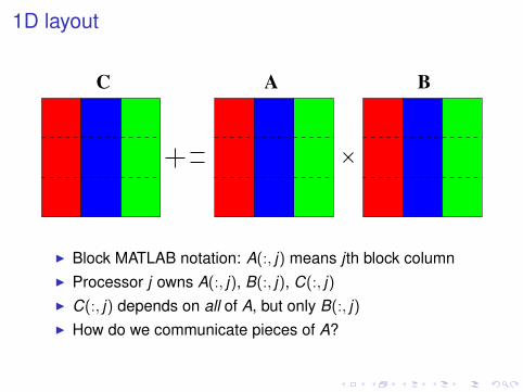
1D layout

BC A

I Block MATLAB notation: A(:, j) means j th block columnI Processor j owns A(:, j), B(:, j), C(:, j)I C(:, j) depends on all of A, but only B(:, j)I How do we communicate pieces of A?

1D layout on bus (no broadcast)

BC A

I Everyone computes local contributions firstI P0 sends A(:,0) to each processor j in turn;

processor j receives, computes A(:,0)B(0, j)I P1 sends A(:,1) to each processor j in turn;

processor j receives, computes A(:,1)B(1, j)I P2 sends A(:,2) to each processor j in turn;

processor j receives, computes A(:,2)B(2, j)

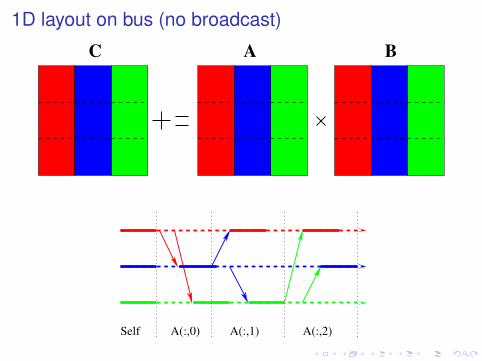
1D layout on bus (no broadcast)

Self A(:,1) A(:,2)A(:,0)

C A B

1D layout on bus (no broadcast)

C(:,myproc) += A(:,myproc)*B(myproc,myproc)for i = 0:p-1for j = 0:p-1if (i == j) continue;if (myproc == i) isend A(:,i) to processor j

if (myproc == j)receive A(:,i) from iC(:,myproc) += A(:,i)*B(i,myproc)

endend

end

Performance model?

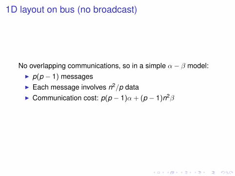
1D layout on bus (no broadcast)

No overlapping communications, so in a simple α− β model:I p(p − 1) messagesI Each message involves n2/p dataI Communication cost: p(p − 1)α + (p − 1)n2β

1D layout on ring

I Every process j can send data to j + 1 simultaneouslyI Pass slices of A around the ring until everyone sees the

whole matrix (p − 1 phases).

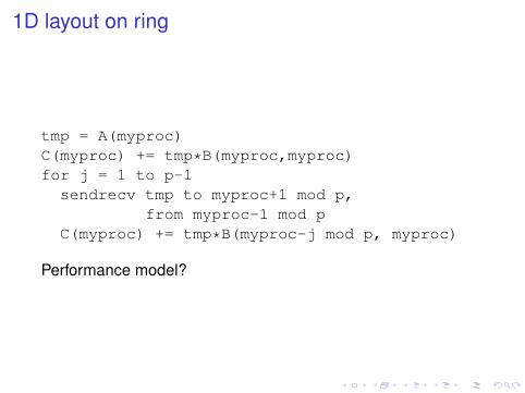
1D layout on ring

tmp = A(myproc)C(myproc) += tmp*B(myproc,myproc)for j = 1 to p-1sendrecv tmp to myproc+1 mod p,

from myproc-1 mod pC(myproc) += tmp*B(myproc-j mod p, myproc)

Performance model?

1D layout on ring

In a simple α− β model, at each processor:I p − 1 message sends (and simultaneous receives)I Each message involves n2/p dataI Communication cost: (p − 1)α + (1− 1/p)n2β