Lecture 19. The Method of Zs 

When problems get complicated numerical complexity makes computa7on SLOW 

The method of Zs speeds the computa7on up 

We will eventually look at the third problem of problem set 5  which is computa7onally imprac7cal (at least in Mathema7ca) without Zs 

1 

We set this in the context of Hamilton’s equa7ons with nonholonomic constraints 

I generally replace connec7vity constraints with pseudononholonomic constraints 

When I do this we recall that we can write 

€

˙ q i = S ji u j

The momentum can be wriIen in terms of uj. 

€

pi =∂L∂ ˙ q i

/.{˙ q i → S ji u j}

where I am borrowing Mathema7ca’s subs7tu7on operator 

2 

3 

The game is to isolate the us, wri7ng the deriva7ves as coefficients 7mes us   

I will denote the coefficients in the momentum   (Hamilton and reduced Hamilton) equa7ons by Zs  

This is going to seem a wee bit weird  Bear with me.  It’ll make sense eventually 

We note that pi is linear in uj, which we can write as 

€

pi = Zijuj

4 

We can obtain the Zs from the usual momentum expression 

€

pi = Mij ˙ q j = Mik ˙ q k = MikS jku j ⇒ Zij = MikS j

k

or 

€

Zij =∂pi∂u j

The laIer is oQen easier 

5 

€

Zij = MikS jk

It is clear from the expression 

that Z does not depend on u 

6 

We already have the equa7ons for the evolu7on of q:  

€

˙ q i = S ji u j

Hamilton’s equa7ons become 

€

˙ p i = Zij ˙ u j + ˙ Z ijuj =

∂L∂qi + Qi

where any explicit   

€

˙ q i = S ji u j

We need to replace 

€

˙ Z ij =∂Zij

∂qk ˙ q k =∂Zij

∂qk Smk um

7 

So that we have Hamilton’s equa7ons in the form 

€

Zij ˙ u j +∂Zij

∂qk Smk umu j =

∂L∂qi + Qi

Remember that these are not actually correct   because I have not wri@en the Lagrange mulBpliers 

€

Zij ˙ u j +∂Zij

∂qk Smk umu j =

∂L∂qi + Qi + λkCi

k

is the correct form 

8 

We have learned to mul7ply by S to obtain the correct form  the reduced Hamilton’s equa7ons 

€

Zij ˙ u jSni +

∂Zij

∂qk Smk umu jSn

i =∂L∂qi Sn

i + QiSni

We need to solve these simultaneously with the q equa7ons 

€

˙ q i = S ji u j

9 

€

∂L∂qi

is, formally, a terribly complicated expression 

€

∂L∂qi =

12

˙ q p∂M pq

∂qi ˙ q q − ∂V∂qi

€

∂L∂qi

=12Smpum

∂Mpq

∂qiSnqun − ∂V

∂qi

However, if we relegate the connec7vity constraints to the pseudononholonomic world  most of the deriva7ves of M are zero, and it is not at all bad    We will see this in context 

10 

€

Zij ˙ u jSni +

∂Zij

∂qk Smk umu jSn

i =12

Smp um ∂M pq

∂qi Snqun −

∂V∂qi

Sn

i + QiSni

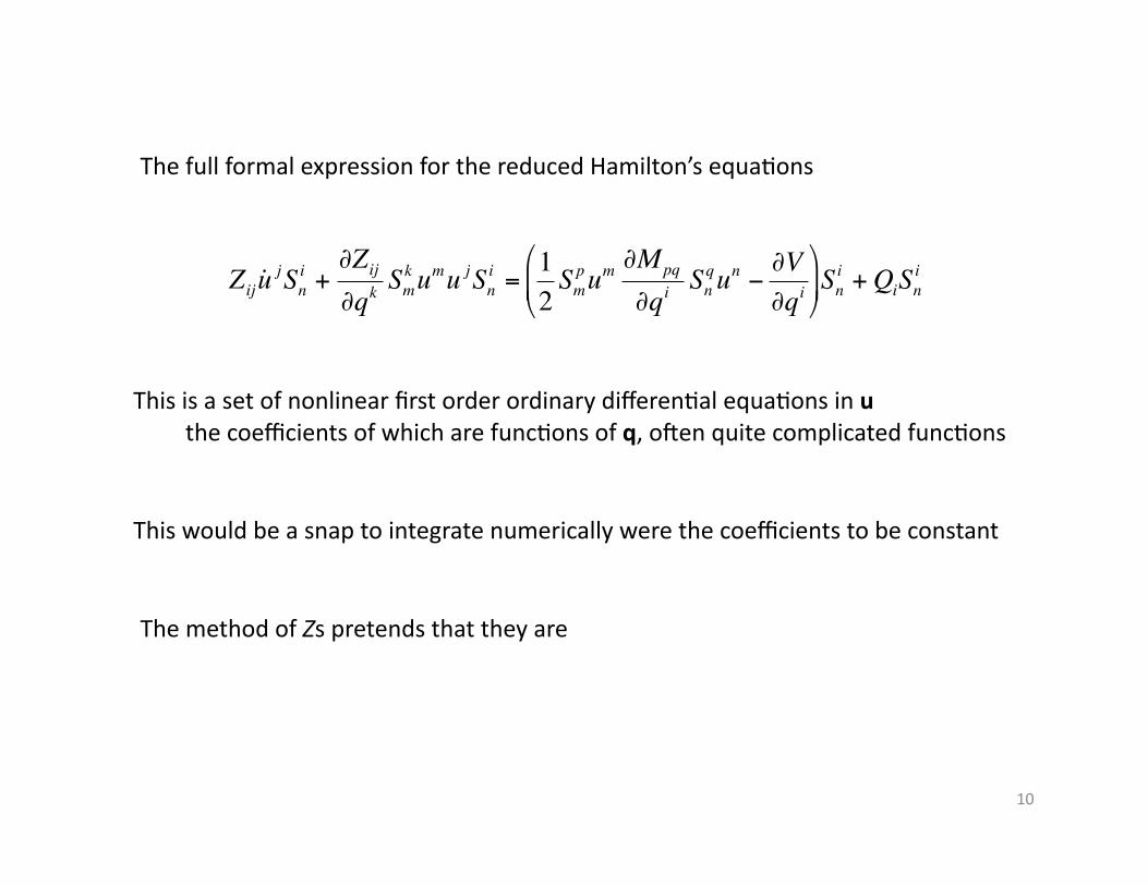
The full formal expression for the reduced Hamilton’s equa7ons 

This is a set of nonlinear first order ordinary differen7al equa7ons in u  the coefficients of which are func7ons of q, oQen quite complicated func7ons  

This would be a snap to integrate numerically were the coefficients to be constant 

The method of Zs pretends that they are 

11 

I have adapted the method of Zs from Kane and Levinson’s 1983 paper, cited in the text 

Their work used Kane’s method, which I explore in the text, but not in class 

My method of Zs is not as complete as it might be,   because I allow some of the coefficients to remain as explicit func7ons of q 

This relies on  

€

∂L∂qi

and Sij actually being preIy simple func7ons of q 

(and also the generalized forces) 

12 

€

ZijSni ˙ u j +

∂Zij

∂qk Smk Sn

i umu j =∂L∂qi Sn

i + QiSni

Write Hamilton’s equa7ons as follows 

We replace the Z variables by constants 

€

Zij → Tij , ∂Zij

∂qkSmk → Tijm

€

TijSni ˙ u j + TijmSn

i umu j =∂L∂qi Sn

i + QiSni

This choice of subs7tu7ons aligns with Hamilton’s equa7ons, not the reduced equa7ons 

13 

Of course, they are not constants, so we have to add algebraic equa7ons  to our system to allow us to calculate them as we go forward 

€

Tij = Zij qk( ), Tijm =

∂Zij qp( )

∂qkSmk qq( )

That has been a lot to digest, and we’ll go through an example shortly 

Let me try to summarize this first 

14 

the simple holonomic constraints 

generalized coordinates 

Lagrangian 

nonholonomic and pseudononholonomic constraints 

Hamilton’s equa7ons 

Start from square one 

€

˙ q i = S ji u j

introduce the Zs 

reduced Hamilton’s equa7ons with Zs 

generalized forces 

15 

Consider the liIle sphere on the big sphere — both free to roll 

16 

How do we set this up? 

Set the K axis of the big sphere horizontal as before for rolling 

I can choose the iner7al axis such that the small sphere is on the i axis  without loss of generality  

If all I care about is the ball rolling down star7ng from rest  then the simplest thing to do is but its K axis horizontal as well 

17 

18 

It might be fun to start the ball rolling on a line of la7tude 

The easiest way to do that is to put the K axis on a line of longitude  which we can do by the proper choice of φ and θ. 

We want K to be 

€

K 2 =

−cosζcosη−cosζsinηsinζ

Pick 

€

φ2 =η+π2

, θ2 = ζ −π2

19 

20 

Go to Mathema7ca to look at this