lecture 2: mapping in matlab
TRANSCRIPT

Lecture 2: Mapping in Matlab
James P. LeSageUniversity of Toledo
Department of EconomicsToledo, OH 43606
March 2004

1 Introduction
Recent developments in computer gaming have lead to powerful computergraphics hardware becoming part of basic laptop and desktop computers.This graphics hardware can draw thousands of polygons on computer screensin a fraction of a second, allowing software that reads thousands of mappolygons from ESRI’s ArcView map file format known as shape files intothe Matlab software environment for graphical presentation. An under-lying public domain library of c/c++ language Application ProgrammingInterface (API) functions known as shapelib was used along with the Matlabc/c++ language interface labelled C-MEX by the MathWorks. The shapelibfunctions include one API for processing, manipulating and extracting mappolygon information from ESRI’s shape files, and another API for process-ing, manipulating and extracting database information from associated files.The associated data information contains sample data observations for eachregion or polygon area on the map, that can be used in spatial econometricmodeling.
We focus on design and implementation considerations that arose in pro-ducing Arc Mat for the Matlab environment, but many of these issues wouldalso apply to implementing similar functionality in other software environ-ments for spatial statistical modeling such as R/Splus, Octave or SciLab.Most statistical software environments include functions for plotting poly-gons that would allow the underlying map polygons from ArcView mappingsoftware to be presented within the statistical software environment, as wehave done for the case of Matlab. This results in presentation quality withinthe statistical software environment that is nearly identical to that of the Ar-cView software mapping environment. An important advantage of operatingin the statistical software environment is that powerful spatial econometricmodeling tools are available in these environments.1
An alternative to the design approach taken here is the one utilized byGeoDA (Anselin et. al, 2002), which is freestanding and does not requirea specific GIS system. GeoDa runs under the Microsoft Windows operat-ing system and provides an interactive environment that combines mapswith statistical graphics, using dynamically linked windows. GeoDa ad-heres to ESRI’s shape file as the standard for storing spatial information. Ituses ESRI’s MapObjects LT2 technology for spatial data access, mappingand querying and provides functionality through the use C++ classes with
1For examples see LeSage’s public domain Spatial Econometrics Toolbox or Pace’sSpatial Statistics Toolbox in the case of Matlab, or Bivand’s spdep for the R/Splus envi-ronment.
1

associated methods. Use of C++ programs for spatial statistical modelingeliminates reliance on software such as Matlab or R/Splus, but requires thatusers learn a new statistical software interface. Reliance on software suchas Matlab or R/Splus has the advantage that thousands of user-contributedfunctions for statistical and spatial statistical modeling already exist forthese environments. In contrast, the approach taken by GeoDa requiresthat users rely entirely on the set of statistical functions selected by de-velopers for inclusion in the new environment, or develop their own C++modeling functions within the new environment. GeoDa currently does notcontain specific techniques to analyze geostatistical or point pattern data,but these are planned as a future development.
Yet another approach would be to utilize operating system specific func-tionality for linking programs such as DLL’s in the case of Windows, or othersuch functionality that would allow use of one program as a compute enginefor statistical calculations and ESRI’s ArcView software as a graphics enginefor map presentation. The drawback to this approach would be that designand implementation would be specific to an operating system and perhapsa hardware platform. Another difference between this approach and the onedescribed here is that development of compiled language code would rep-resent the majority of the system implementing this type of approach. Incontrast, the majority of the Arc Mat Toolbox consists of Matlab programsthat can be developed and debugged in an interactive programming environ-ment, avoiding the edit-test-debug development loop common to compiledlanguage program development.
Part of this paper focuses on a set of Matlab development tools andsupport functions for Graphical User Interface (GUI) program development,that was used to produce an interface to the underlying Matlab mappingfunctions. While this is specific to the Matlab environment, similar GUIfunctionality exists in the other statistical software mentioned above. Ourimplementation calls a single function using the command-line which createsa GUI interface. This interface presents the map as well as pull-down menusand other GUI tools for changing map properties such as: the color scheme,legend, variables mapped, as well as zooming in and out on sub-regionsof the map. Readers familiar with the ArcView program will recognizethat this same type of functionality is available in ESRI’s ArcView softwareenvironment.
The ability to provide mapping support for spatial econometric and spa-tial statistical analysis in a single software environment avoids the need totransfer files between different software programs. Practitioners involved indevelopment of spatial econometric models can examine model results such
2

as residuals, predicted values, observations identified as candidate outliers,etc., using a single function call that transfers matrices or vectors containingmodel results to the GUI mapping environment for visualization.
Another aspect of the tools described here is that they can be used toextract GIS information for use in other mapping software that presentlyexists for the Matlab environment. An extensive set of functions labelledGeoXP described in (Heba Malin, Thomas-Agnan, 2002) has been devel-oped for both Matlab and R/Splus software environments. The polygoncoordinates produced by the c/c++ language interface of Matlab describedhere can be used to provide support for this library of functions.
Section 2 of the paper describes software issues related to the underylingfile-transfer mechanism used to extract both mapping and database infor-mation from the ArcView files. The Matlab mapping software functions andissues pertaining to design of the GUI interface are set forth in section 3.Section 4 discusses usage issues related to the mapping functions and spa-tial econometric analysis. Focus is on situations where information from theArcView shape files is useful in spatial econometric and spatial statisticalmodeling.
2 Underlying algorithms and design for extractingand importing shape file information into Mat-lab
The Matlab programming environment consists primarily of a command-line interface, where commands input using the keyboard or files containingcommand instructions are processed by a combined interpreter and just-in-time compiler. As the name Matlab suggests, the programming environmentis based on matrix and vector constructs. User-written functions representa key feature of the software environment, and these can be written in theMatlab programming language as well as external languages such as c, c++,or FORTRAN. Other statistical software environments such as R/Splus,Octave and SciLab operate in a similar fashion and provide an externallanguage interface.
External language programs must be compiled and linked to the Mat-lab program execution environment using an interface gateway known asC-MEX or F-MEX, in the case of c/c++ or FORTRAN languages. C-MEXfiles are written in the c/c++ language, and in the case of our file interfaceto the ArcView shape files, they represent an intermediate file that translatesinput arising from a function call executed within Matlab into appropriate
3

calls to a public domain library of functions known as shapelib. This libraryprovides a series of API functions for reading, writing and extracting infor-mation from ArcView shape files. The term shape file is typically used torefer to a number of files that are generated by ArcView mapping projects,leading us to use the plural term shape files. These files can contain informa-tion on sample data stored in a database (dbf ) file format, map projections,map polygons, and a host of other things related to ArcView projects. Theshapelib functions provide an API for manipulating, reading and writingboth mapping and database information from the ArcView formatted files.
We rely on a single Matlab function written in the native programminglanguage that is named shape read and takes a single argument containinga string with the basename of the shape files to be imported into Matlab. Asalready noted, the term ‘shape file’ is a misnomer since this is a reference toat least three different files with the same basename but different filenameextensions, .shp, .shx and .dbf. There are other possible files such as thosecontaining map projection information that have a .prj extension, that arenot currently used in our implementation.
The shape read function calls underlying C-MEX functions that callthe shapelib API functions to: 1) read polygon information, and 2) extractdatabase information. In addition to functionality for extracting informa-tion, the shapelib API also contains functions for performing calculationsusing information from the ArcView formatted files and writing new ahapefiles that might contain transformed polygon and database information. Weuse API functionality to calculate polygon centroid coordinates, which rep-resent a key variable used to construct spatial weight matrices in spatialmodeling.
The single Matlab function carries out error checking regarding file avail-ability and combines all information returned by calls to different compliedAPI functions into a single Matlab ‘structure’ variable. Structure variablesrepresent a container with ’fields’ that can consist of strings, vectors, scalarsand matrices of varying dimensions and variable types. This provides aconvenient way to return large amounts of heterogenous information fromfunction calls and passing this information between functions. Individualfields in the structure variable are referenced using a ‘.’ and the field name.An example of using the shape read function would be:
filename = ‘africa’;results = shape_read(filename);npolygons = results.npoly;
The structure variable ‘results’ contains information that is available
4

through ‘.’ referencing the field names, as illustrated by transferring thescalar field ‘.npoly’ indicating the number of polygons in the ‘africa’ shapefile to another scalar variable named ‘npolygons’. Documentation for theshape read function provides complete information on fields contained inthe ‘results’ structure variable. This can be viewed in the Matlab com-mand window environment by typing: ‘help shape read’, which returns theinformation shown below.
PURPOSE: reads an arcview shapfile and returns a structure
that can be used by make_map(), arc_histmap(), moran_map()
and other Arc_MAT mapping functions
-------------------------------------------------------------------------
USAGE: results = shape_read(filename)
where: filename = an arcview shape file name without the extension
-------------------------------------------------------------------------
Returns: a structure variable:
results.npoly = a scalar with # of polygon regions (observations) on the map
results.nvars = # of variables from the .dbf file [should = the length(vnames)]
results.nobs = # of observations from the dbf file [should = npoly]
results.xmin = an nobs-vector of minimum longitude for each region
results.xmax = an nobs-vector of maximum longitude for each region
results.ymin = an nobs-vector of minimum latitude for each region
results.ymax = an nobs-vector of maximum latitude for each region
results.nvertices = an nobs-vector of # of vertices for each region
results.nparts = an nobs-vector of # of parts for each region
results.xc = an nobs-vector with x-centroid for each polygon/region
results.yc = an nobs-vector with y-centroid for each polygon/region
results.data = (an nobs=npoly by nvars) matrix of sample data observations
for each polygon/region
results.vnames = variable names for data vectors from the .dbf file
results.x = an (n by nvertices) vector of polygon points, with NaN separators
results.y = an (n by nvertices) vector of polygon points, with NaN separators
Users need not be concerned with manipulating the information con-tained in the structure variable to produce map visualizations. The structurevariable can simply be passed on to a mapping function, which will intel-ligently decipher information from the various fields required to producethe GUI interface containing the map and related map legends or statisti-cal graphs. However, extracting the data information in the field ‘.data’ aswell as centroids of the map regions contained in the fields ‘.xc’ and ‘.yc’ isnecessary to use this information in spatial econometric modeling.
A specific example of the simplest possible way to produce a map isshown below:
5

filename = ‘..\shape_files\china’;
results = shape_read(filename);
arc_histmap(results.data,results);
This would produce a mapping GUI containing a map of China thatpresents the first variable vector in the matrix stored in results.data. TheGUI provides a ‘pull-down menu’ that allows other variable vectors to bepresented on the map. These variables are labelled with names constructedfrom the ‘.vnames’ field obtained from the database (.dbf) component ofthe shape files. Before turning attention to usage of the mapping GUIfunctions, we discuss design considerations related to plotting and graphicalhandling of the map polygons embodied in a function named make map.A description of the GUI mapping interface created by various mappingfunctions that make up the Arc Mat Toolbox is in the next section.
2.1 Plotting map polygons
Recent developments in computer gaming have resulted in inexpensive lap-top and desktop computers containing fairly robust graphics hardware thatis capable of rapidly placing thousands of filled polygons on the display.
A general utility function was created to plot the polygon informationcontained in the ‘results’ structure and return a structure variable containing‘graphics handles’ to each polygon and its possible parts. The term ‘graphicshandles’ is used by the MathWorks to refer to graphical objects that containsinformation about graphics elements including such things as figure windowcharacteristics (e.g., window size, positioning, aspect ratios), polygons, axes,points, and text fonts. These graphical objects can be manipulated withmessages to alter the characteristics of almost all aspects of a graphics figurewindow and its component parts.
The polygon structure used by ArcView can be represented as two vec-tors containing latitude and longitude coordinates for each map region,where individual polygons are indicated by a separator symbol. However,a complication arises with respect to map features such as lakes and rivers,which is handled through the use of a sub-structure called a polygon part.Without getting into detail, parts can be recognized by a reversal of thecoordinate directions. Knowledge of this organization scheme can be usedto appropriately parse the vectors of polygon coordinates and plot these in afigure window. This work is done by a utility function named make map,
6
which takes the ‘results’ structure returned by the shape read function andreturns another structure. This contains a pointer to an invisible map fig-ure along with a multi-dimensional graphics handle structure ‘poly.handles’taking the form: poly(i).handles(k), where i references each polygon as-sociated with a map region, and k ranges over possible ‘parts’ associatedwith each region.
The function make map produces an invisible graphics figure, whichcan be manipulated using the graphics handles. The motivation for creat-ing an ‘invisible’ graphics figure containing map polygons at this point is toallow simultaneous presentation of the map figure as well as the associatedmap legend figure and various pull-down menus that constitute the mappingGUI. Individual polygons representing map regions can be made visible orinvisible, the color scheme as well as polygon fill colors and numerous othercharacteristics of the polygons can be manipulated using Matlab functionsthat provide support for manipulation of a wide array of the graphic ob-ject properties contained in the handles. Note that R/Splus also utilizes anobject-oriented approach to graphics, which should allow a similar approachto that taken here. There are also numerous graphical software environ-ments for languages such as c/c++ and FORTRAN for various operatingsystems such as Windows and Linux that implement object-oriented graph-ics developed using a similar philosophy.
The design intention is that the make map function would be calledonce at the beginning of the actual GUI-based mapping functions. Afterthis call, the component functions that make up the graphical user-interfaceoperate on the graphics handles contained in the structure variable ‘poly’that are passed to these sub-functions. Changing the properties and statesof the polygons by manipulating the structure variable elements containinggraphics handle references or pointers to each map polygon represent themethod used to carry out mapping operations. For example, a pull-downmenu option might allow the user to change the color scheme of the mapto reflect a gray-scale map rather than a color-coded map. This would beaccomplished by the sub-function through operation on the graphics handleobject properties contained in the multidimensional ‘poly’ structure variable.
Another important design consideration is that we plot the map polygonsonly once to produce speed in the graphical presentation. This is particularlyimportant to facilitate functionality that allows the user to ‘zoom’ in andout on sub-regions of the map. During these operations, the same polygonsoriginally placed in the graphic figure window are utilized by changing theirstate from visible to invisible when map zooming operations takes place.The state of map polygons outside the sub-region of interest is changed from
7

visible to invisible, but these polygons are never destroyed. This eliminatesthe need to re-draw the polygons which can be computationally intensive formaps involving a large number of polygons. As an example of the speed, thetime required to read the ArcView shape file information by the functionshape read for a file containing 3,111 US counties was 2.0 seconds on aDell Pentium III-M (Centrino) 1.6 Ghz laptop. The time taken to plot themap polygons and form the graphics handle structure variable taken bythe function make map was 1.60 seconds, with 1.27 seconds of this timerequired to plot the polygons, and 0.33 seconds taken to form the polygonhandles structure ‘poly’. The map zooming operation for this case of 3,111polygons takes around 0.3 seconds, which suggests that re-drawing the mappolygons during zooming operations would dramatically slow the interactivepresentation requiring 1.27 seconds in place of the 0.3 seconds, or a factorof four slowdown.
One advantage of operating in a high-level statistical software program-ming environment already noted is the availability of econometric, statisticaland spatial econometric modeling functions. Another advantage is portabil-ity across different operating systems and hardware environments such asUNIX, MS-Windows and Apple OSX that most statistical software includ-ing Matlab supports. A third advantage is that the statistical software pro-vides an intelligent interface to underlying hardware and software graphicsfunctionality. For example, Matlab automatically handles numerous defaultdecisions regarding hardware versions of OpenGL. Matlab detects the hard-ware version if it is available, and if a hardware version of OpenGL is notavailable, Matlab uses a software version of these low-level graphics func-tions. This default behavior can be overwritten by the programmer, butreliance on this allows underlying design decisions to be implemented acrossmultiple hardware and operating system platforms in a consistent fashion.To illustrate the complexity of dealing with software/hardware graphics pe-culiarities, consider the following criterion used by Matlab when dealingwith the decision to use OpenGL versus other underlying graphics hardwareor software functions.2 Matlab selects OpenGL if:
The host computer has OpenGL installed and is in True Color mode(OpenGL does not fully support 8-bit color mode).
The figure contains no logarithmic axes (logarithmic axes are not sup-ported in OpenGL).
Matlab would select zbuffer based on figure contents.2This information was taken from documentation in Matlab version 6.5
8

Patch objects faces have no more than three vertices (some OpenGLimplementations of patch tesselation are unstable).
The figure contains less than 10 uicontrols (OpenGL clipping arounduicontrols is slow).
No line objects use markers (drawing markers is slow).
Phong lighting is not specified (OpenGL does not support Phong light-ing; if you specify Phong lighting, Matlab uses the ZBuffer renderer).
The point here is that developing mapping functionality in a native lan-guage environment such as c/c++ or FORTRAN would require a series ofknowledgable decisions about the inherent strengths and weaknesses of un-derlying graphics hardware/software libraries. This would seem to be thesituation confronted by the GeoDA project, which can be avoided whenrelying on high-level languages such as R/Splus or Matlab.
Another place where high-level language functionality comes into playfor mapping is automatic control of modes related to data and plot box as-pect ratios. The Arc Mat Toolbox allows users to zoom in on sub-regions ofthe map figure, which can produce distorted images unless care is taken topreserve aspect ratios. Our current implementation utilizes the map projec-tion present in the ArcView shape files. ESRI provides a number of toolsto change map projections and newer versions the the software produce acomponent shape file with the ‘.prj’ extension that contains projection infor-mation. There are a host of design issues related to implementing facilitiesfor changing mapping projections. Starting with a global map, zoomingin on a sub-region of the world requires that care be taken to change themap projection. A commercial Mapping Toolbox is available from the Math-Works that contains numerous functions for changing polygon coordinatesto reflect alternative map projections. There is also a public domain Matlabmapping toolbox M map that also contains projection functions.
We note that the objective of the Arc Mat Toolbox is not cartographicreality, but rather comparative visualization of sample data relationshipsthat may exist between regions. Visualizing a cluster of residuals that takeon similar values to those from neighboring observations does not requirehigh precision projections. Rather, emphasis is on preserving the aspectratio of the initial projection so as not to disorient the user when zoomingin or out on the map. In theory, map projection transformations of thepolygon coordinates could be incorporated as an option in Arc Map, butthis is not currently implemented. We note that our earlier discussion of
9

the time required to plot a large number of polygons suggests a trade-offbetween speed and cartographic reality. Changing from the initial mapprojection to a new one would require another call to make map to draw anew set of polygons and form graphics handles based on these transformedpolygons. The reported timing tests suggest this would slow map zoomingoperations by a factor of five times, when we take into account time neededto plot the polygons as well as reform the graphic handles structure. Futureadvances in graphics hardware and software should change the nature of thistrade-off, perhaps allowing a pull-down menu for changing map projections.Automatic changes in projection based on zooming in or out on map sub-regions would also be possible, but represent the most compute intensiveapproach.
3 A GUI interface for mapping in Matlab
The Matlab programming environment provides a host of functions that canbe used to produce a graphical user interface. Our discussion here focuses onthe Matlab environment, but many of the design considerations would alsoapply to other statistical software environments. A program that utilizesthe GUI functions can be constructed to allow a single function call fromthe Matlab command window, or a file containing Matlab commands tocreate the GUI interface. This Arc Map design decision was motivated bythe need to allow users to pass matrices or vectors returned by functionsfor spatial econometric analysis to produce a map. A number of differentmapping GUI’s exist as separate functions that produce different types ofmaps relevant for spatial statistical analysis.
Calling one of the mapping GUI functions turns control over to themapping GUI, allowing various pull-down menus to be used to control char-acteristics of the map presentation. For example, pull-down menus allowthe user to change: color schemes, variable selection from the input matrix,zooming of sub-regions on the map, choice of the number of legend cate-gories, and labelling of the map polygons. On exit from the mapping GUI,control is returned to Matlab where further spatial econometric analysis orcalls to another another type of GUI mapping function could be undertaken.
We provide an overview of the different types of GUI mapping functionscurrently available in Arc Map, followed by sub-sections describing each ofthese in more detail.
The basic mapping function is named arc histmap, which produces amap based on an n by k matrix input, where n denotes the rows in the
10

matrix which represent regions or observations, and k denotes the numberof columns in the matrix which contain variable vectors. The mapping GUIproduces a map of the first variable vector (column) of the input matrix inone figure window along with a histogram showing the distribution of theobservation values in another figure window. Figure 1 provides an illustra-tion of this type of map, with the associated legend shown in Figure 2. Themap displays population growth of provinces in China over the 1980 to 1995period, allowing easy identification of high versus low growth provinces.
A second type of mapping GUI is the Moran scatterplot that depicts avariable y on the horizontal axis with the average of “neighboring region”values for the variable y on the vertical axis, as a scatter of points. The aver-ages for neighboring regions are constructed using an n by n spatial weightmatrix W , that contains non-zero entries in the i, jth position if observationj represents a “neighboring region”, and zeros on the main diagonal. Forthe case of neighboring regions defined using a spatial contiguity, the matrixW could be constructed by placing values of unity in positions i, j, where jindicates regions that have borders touching region i. This matrix is thenrow-standardized to have row-sums of unity. The matrix product Wy thenproduces an average of the values from regions meeting this definition ofneighbors. Various functions for producing spatial weight matrices based oncontiguity, nearest neighbors, and distance are a part of the Spatial Econo-metrics Toolbox and the Spatial Statstics Toolbox. Since Matlab representsa programming environment, users are free to construct spatial weight ma-trices based on other criterion that appropriately define the structure ofconnectivity relationships between regions for their particular problem.
Figure 3 shows the Moran scatter plot where the population growthrates in the vector y described above have been transformed to deviationfrom the means form. This allows the population growth rates shown onthe horizontal axis for each region to be expressed as positive if they abovethe overall average population growth rate, or negative if they are belowthe average. The vertical axis was constructed using a first-order contigu-ity spatial weight matrix that produces average growth rates of neighboringprovinces, again in deviation from the means form. The four color-codedquadrants in the scatter plot depict: 1) regions where higher than averagegrowth rates are associated with an average of neighboring region growthrates that are also higher than average (the red points), 2) regions wherelower than average growth rates are associated with an average of neighbor-ing region growth rates that are also lower than average (the cyan points) 3)regions where lower than average growth is associated with neighboring re-gions having higher than average growth (the green points) and, 4) regions
11

where higher than average growth is associated with lower than averagegrowth in neighboring regions (the purple points).
The map figure depicts regions using the color coding from the scatterplot, and numerical labels can be provided as an option in both figures toallow identification of the growth rates associated with each region versusthat of neighboring regions. This type of scatter plot is frequently used toassess the extent to which sample data observations exhibit spatial depen-dence. The presence of a large number of red points in the first quadrant areindicative of strong spatial association since provincial growth rates shownon the horizontal axis are positively associated with the average growth rateof neighboring provinces. Similarly, a large number of cyan points in thethird quadrant point to positive spatial association since they indicate thatthe value of the variable on the horizontal axis is positively associated withthe average value from neighboring regions. In contrast, points depicted asgreen and purple reflect negative spatial association, since these are obser-vations that are inversely related to the average of neighboring observations.
A third use for the mapping GUI functions is something labelled sar map,where SAR stands for a spatial autoregressive econometric model. The spa-tial autoregressive model represents a variant of simple regression: y =Xβ + ε which adds an additional explanatory variable to the model, Wy,that reflects a spatial lag: y = ρWy + Xβ + ε.
This function allows the user to select sub-regions on the map for whichspatial autoregressive model estimates of the parameters β and ρ as wellas the noise variance estimate σ2
ε , log-likelihood function value, R2 measureof fit, and other information will be produced. The estimates for a sub-region are presented alongside those for the entire sample. This allows anassessment of local variability in the nature of the underlying linear spatialautoregressive relationship of interest.
This type of GUI mapping interface illustrates a distinct advantage ofMatlab over more conventional GIS mapping environments, in that spatialeconometric methods can be used as part of the map interface. Solving formaximum likelihood estimates of basic spatial regression models providessome computational challenges when the problem involves large samples.This makes it difficult to provide estimation functionality in mapping soft-ware, which would need to provide sparse matrix functionality as well asalgorithms for numerical linear algebra. In contrast, this functionality isalready provided by the public domain Spatial Econometrics and SpatialStatistics toolbox functions for the Matlab environment. Similar spatialeconometric modeling functionality exists in spdep for the R/Splus softwareenvironment.
12

The toolbox functions utilize sparse matrix algorithms available in Mat-lab as well as computationally efficient algorithms suggested in Barry andPace (1999) for computing the log-determinant of an n by n matrix, and avectorized approach to producing maximum likelihood estimates describedin Pace and Barry (1997). Taken together, these allow maximum likeli-hood estimates to be produced in one or two seconds for problems involvingover 3,100 US counties. This speed allows the initial global estimates for amodel to be shown in a graphics window and rapid updating of estimates forsub-regions selected using the GUI interface. Single regions can be addedor subtracted from the sub-region selection set to test for influential obser-vations. Figure 5 shows the selection map, where a sub-sample of 1,257observations (highlighted) in the center of the contiguous US states havebeen selected from the total of 3,111 county-level observations.
Figure 6 shows the graphics window that presents global estimates along-side those from the selected sub-region for comparison. The model used toproduce this illustration represents a spatial autoregressive ‘growth regres-sion’, that relates employment growth rates over the 1980 to 1990 period toa host of county-level characteristics. Coefficients with a positive sign indi-cate that the associated characteristics promote higher employment growthrates, whereas negative signs suggest the converse.
As an example of how the comparative estimates and associated t−statisticsmight be useful, consider the coefficient on college, where this variable re-flects the percent of population aged 25 and over holding college degreesas their highest level of educational attainment. For the global sample,the coefficient is not statistically significantly different from zero, whereasthe sub-region in the center of the US produced a negative and significantestimate.
Having provided a brief introduction to the various types of GUI map-ping functions, we provide a more detailed discussion regarding each of thesein the following sub-sections.
3.1 The arc histmap function
This function provides basic mapping of a matrix where rows of the matrixinput are associated with the map regions contained in the ArcView shapefile and each column represents a different variable. Two associated figurewindows are displayed, one containing a map of the observation values foreach region, and the other a histogram showing the distribution of thesevalues. These figure windows can be resized and moved independently ofeach other, with the legend figure possibly overlaid on top of the map figure.
13
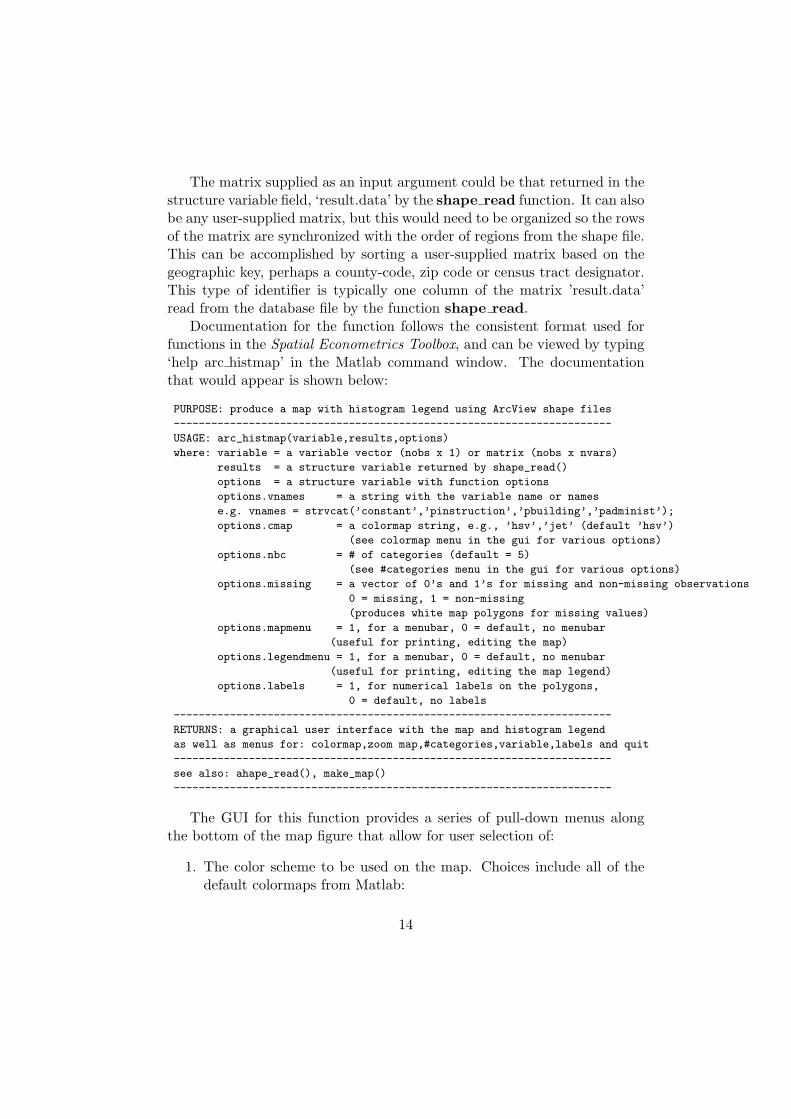
The matrix supplied as an input argument could be that returned in thestructure variable field, ‘result.data’ by the shape read function. It can alsobe any user-supplied matrix, but this would need to be organized so the rowsof the matrix are synchronized with the order of regions from the shape file.This can be accomplished by sorting a user-supplied matrix based on thegeographic key, perhaps a county-code, zip code or census tract designator.This type of identifier is typically one column of the matrix ’result.data’read from the database file by the function shape read.
Documentation for the function follows the consistent format used forfunctions in the Spatial Econometrics Toolbox, and can be viewed by typing‘help arc histmap’ in the Matlab command window. The documentationthat would appear is shown below:
PURPOSE: produce a map with histogram legend using ArcView shape files
----------------------------------------------------------------------
USAGE: arc_histmap(variable,results,options)
where: variable = a variable vector (nobs x 1) or matrix (nobs x nvars)
results = a structure variable returned by shape_read()
options = a structure variable with function options
options.vnames = a string with the variable name or names
e.g. vnames = strvcat(’constant’,’pinstruction’,’pbuilding’,’padminist’);
options.cmap = a colormap string, e.g., ’hsv’,’jet’ (default ’hsv’)
(see colormap menu in the gui for various options)
options.nbc = # of categories (default = 5)
(see #categories menu in the gui for various options)
options.missing = a vector of 0’s and 1’s for missing and non-missing observations
0 = missing, 1 = non-missing
(produces white map polygons for missing values)
options.mapmenu = 1, for a menubar, 0 = default, no menubar
(useful for printing, editing the map)
options.legendmenu = 1, for a menubar, 0 = default, no menubar
(useful for printing, editing the map legend)
options.labels = 1, for numerical labels on the polygons,
0 = default, no labels
----------------------------------------------------------------------
RETURNS: a graphical user interface with the map and histogram legend
as well as menus for: colormap,zoom map,#categories,variable,labels and quit
----------------------------------------------------------------------
see also: ahape_read(), make_map()
----------------------------------------------------------------------
The GUI for this function provides a series of pull-down menus alongthe bottom of the map figure that allow for user selection of:
1. The color scheme to be used on the map. Choices include all of thedefault colormaps from Matlab:
14
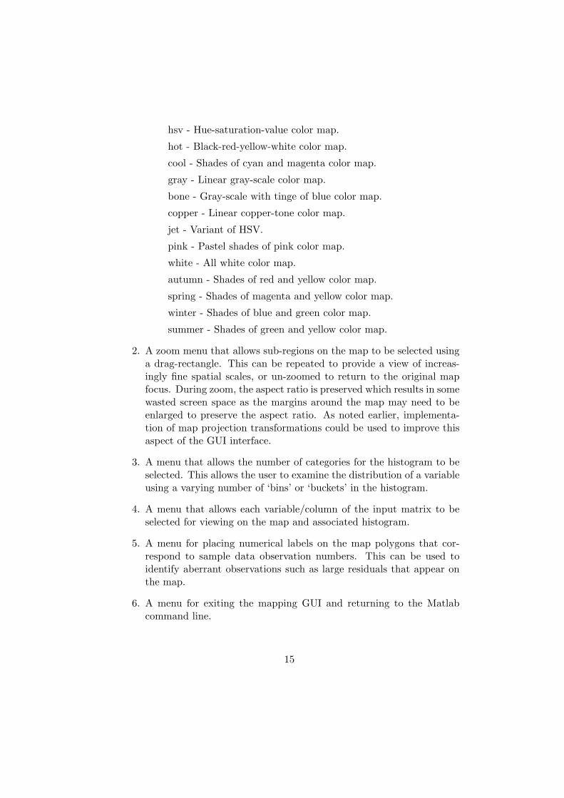
hsv - Hue-saturation-value color map.
hot - Black-red-yellow-white color map.
cool - Shades of cyan and magenta color map.
gray - Linear gray-scale color map.
bone - Gray-scale with tinge of blue color map.
copper - Linear copper-tone color map.
jet - Variant of HSV.
pink - Pastel shades of pink color map.
white - All white color map.
autumn - Shades of red and yellow color map.
spring - Shades of magenta and yellow color map.
winter - Shades of blue and green color map.
summer - Shades of green and yellow color map.
2. A zoom menu that allows sub-regions on the map to be selected usinga drag-rectangle. This can be repeated to provide a view of increas-ingly fine spatial scales, or un-zoomed to return to the original mapfocus. During zoom, the aspect ratio is preserved which results in somewasted screen space as the margins around the map may need to beenlarged to preserve the aspect ratio. As noted earlier, implementa-tion of map projection transformations could be used to improve thisaspect of the GUI interface.
3. A menu that allows the number of categories for the histogram to beselected. This allows the user to examine the distribution of a variableusing a varying number of ‘bins’ or ‘buckets’ in the histogram.
4. A menu that allows each variable/column of the input matrix to beselected for viewing on the map and associated histogram.
5. A menu for placing numerical labels on the map polygons that cor-respond to sample data observation numbers. This can be used toidentify aberrant observations such as large residuals that appear onthe map.
6. A menu for exiting the mapping GUI and returning to the Matlabcommand line.
15

Use of the pull-down menus to select a new colormap, variable, zoomrectangle or number of histogram categories results in returning focus tothe legend figure window so that in cases where this has been overlaid onthe map figure, both figures are visible. There are traditional minimizeand maximize boxes on each figure window, so users can focus on a singlefigure window by minimizing one of the two windows, or expand the viewto full-screen.
Optional input arguments are provided in a structure variable as fields.These allow user input of:
options.vnames - a set of variable names that will appear on the pull-down menu for selecting variables to display on the map.
options.cmap - a color scheme choice to use in the initial map figure.This can be altered in the GUI interface using the pull-down menu.
options.nbc - the number of categories to be used in constructing theinitial histogram and color scheme for the map. This can be alteredin the GUI interface using the pull-down menu.
options.missing - a vector with values of zero and one to indicate mapregions for which there is missing data information. Without thisoptional input vector, the histogram would be distorted by missingvalues. It may be the case that a user-supplied matrix does not containsample data information for all regions on the map that was inputusing the shape read function. This option allows these regions toappear on the map as ‘white’ regions, and these missing values will beignored during construction of the associated histogram figure.
options.mapmenu, and options.legendmenu - a switch that adds a topmenu to the map and legend figures respectively. This menu containsstandard Matlab functions for operating on graphical figures. Forexample, a file menu item allows the figure window to be printed orexported in numerous graphic file formats. Other top menu items allowthe user to add lines and text annotations to the figure windows, anda host of other graphic functionality.
options.labels, which can be used to place numerical labels on the mappolygons. This is useful for checking sample data observations fromthe input matrix that are associated with map regions. This can beturned on or off in the GUI interface using a pull-down menu.
16

The decision to make the top menu an option, rather than the defaultwas made to increase the clarity of presentation, minimizing the amount ofclutter in the GUI interface. Here we see another advantage to operatingin a high-level language environment such as Matlab. The top menu forthe map and legend figures represents a standard property of all Matlabfigure windows. No programming was required to add these features to themapping GUI, simply a change in the state of the figure window properties,achieved with a single call to the functions that operate on the graphicshandles.
A screen capture of the mapping GUI associated with the arc histmapfunction is shown in figure 7. A map of 1,008 Ohio zip code areas is shown,constructed using a matrix containing information on 4th grade studentproficiency test scores for Ohio school buildings. Information from a sampleof nearly 2,000 school building was averaged by zip code area to producethe input matrix. The missing values feature proved particularly importanthere. Some school buildings from the State of Ohio were indeed missingfrom the database provided by the Ohio Department of Education. In othercases, zip code areas had no school buildings or proficiency score informationbecause the zip code area represented a major downtown business districtor industrial/manufacturing region. These regions would not contain schoolbuildings, resulting in missing student proficiency scores that are not missingdue to reporting problems. Users could introduce a binary vector variableto the input matrix to reflect these two scenarios. This variable wouldappear color-coded on the map when selected using the variable selectionpull-down menu in the GUI interface. This might be of interest if therewere concerns about non-reporting school buildings being distributed in aspatially clustered fashion, so that one region of the state exhibited a largeproportion of the reporting problems.
To illustrate the zoom feature, we selected a rectangular sub-region ofthe Ohio zip code areas shown in figure 8, that is centered on Toledo, Ohio.This was done after selecting the ‘zoom’ pull-down menu item labelled ‘selectrectangle’. Both the map figure and associated histogram map legend arerecalculated to reflect the sub-sample of observations selected.3
A clear pattern of lower scores exists for central city school buildings,which is more evident in the zoomed map than that depicting the statewidepatterns. One point to note is that the histogram is based on a number
3Note that the two independent figures showing the map and legend were merged intoa single graphic figure for presentation purposes. Figure 8 does not depict the manner inwhich the map and legend actually appear in the GUI interface.
17

of categories chosen using the GUI interface menu item. This histogrampreserves the number of categories, but places blank bars for values of thevariable that are not represented in the sub-sample. This decision was makefor consistency with the design motivation to not create disorientation ofthe user when viewing sample data information from different perspectives.
3.2 The arc moranplot function
Spatial autocorrelation can be viewed as a map pattern, as well as variousother interpretations. This can be measured using an extension of Pearson’sproduct moment correlation coefficient using a binary spatial weight matrixC, where elements cij = 1 to denote that observation j is relatively closeto location i. This extended correlation coefficient known as the MoranCoefficient becomes:
MC =n∑n
i=1
∑nj=1 cij
∑ni=1
∑nj=1 cij(xi − x)(xj − x)∑n
i=1(xi − x)2(1)
The most common interpretation of spatial autocorrelation is in termsof trends or patterns across a map. In this context, we note that as in thecase of a Pearson product moment correlation coefficient, the value of MCapproaches unity when similar values of the observations tend to cluster onthe map, referred to as positive spatial autocorrelation. Similarly, when thevalue of MC approaches -1, we see dissimilar values clustering on the map,known as negative spatial autocorrelation. A random pattern of values fora variable on the map results in the MC approaching −(1/(n − 1)), whichis asymptotically zero for large values of n.
In contrast to a conventional correlation coefficient, MC is not restrictedto the range [−1, 1], but has a range determined by the minimum and max-imum eigenvalues of the matrix C.
The arc moranplot function attempts to illustrate the strength of spa-tial autocorrelation using a scatter plot of the relation between a variablevector (y − y) measured in deviations from the mean form and the spatiallag of this variable, W (y− y). The spatial weight matrix W differs from thebinary matrix C in that it is row-standardized, so that row-sums are unity.One way to view this scatter plot would be to consider the first-order spatialautoregressive relationship:
(y − y) = ρW (y − y) + ε (2)
Where the disturbance term ε is distributed normally with mean zero andscalar noise variance σ2
εIn.
18

The slope of the Moran scatter plot would be represented by the scalarparameter ρ, so that values near unity indicate high levels of positive spatialautocorrelation. This would correspond to a Moran scatter plot havinga large number of points in quadrant I, where high values of (y − y) areassociated with high values for neighbors W (y− y), and quadrant III, wherelow values are also associated with low values for the neighbors. A valueof ρ near zero points to a random distribution of points across the fourquadrants that make up the Moran scatter plot, pointing to a lack of spatialdependence between observations in the vector (y − y) and the average ofneighboring values W (y− y). Negative values of ρ point to a large number ofpoints in quadrant II, where where low values of (y− y) are associated withhigh values for neighbors W (y− y), and quadrant IV, where high values areassociated with low values for the neighbors.
The ability of the spatial econometric routines to provide maximum like-lihood estimates for the parameter ρ in the first-order spatial autoregressivemodel provides a nice complement to the Moran scatter plot mapping GUI.Another aspect of operating in an environment where spatial econometricroutines are available is the ability to generate sets of different spatial weightmatrices that can be used as an input argument to the Moran scatter plotfunction. For example, one could examine the scatter plot and associatedmap using a spatial weight matrix constructed using first-order neighborsbased on distance or contiguity, as well as higher-order neighbors based oncontiguity or distance. Functions to construct a variety of spatial weightmatrices represent a standard part of the Spatial Econometrics and SpatialStatistics toolboxes are well as the R/Splus spatial functions spdep.
Documentation for the function arc moranplot is shown below:
PURPOSE: produce a map with moran scatterplot using ArcView shape files
----------------------------------------------------------------------
USAGE: arc_moranplot(variable,W,results,options)
where: variable = a variable vector (nobs x 1), which is transformed
to deviations from the mean form by the function.
W = a spatial weight matrix
results = a structure variable returned by shape_read()
options = a structure variable with function options
options.vname = a string with the variable name
options.labels = 1 for labels, 0 = default, no labels
options.mapmenu = 1, for a menubar, 0 = default, no menubar
(useful for printing, editing the map)
options.legendmenu = 1, for a menubar, 0 = default, no menubar
(useful for printing, editing the map)
----------------------------------------------------------------------
RETURNS: a graphical user interface with the map and moran scatterplot
19

as well as menus for: zoom map,labels and quit
----------------------------------------------------------------------
see also: shape_read(), make_nnw(), xy2cont()
----------------------------------------------------------------------
As in the case of the arc histmap function, options are input using astructure variable, and the map and legend menu options are provided aswell as the labelling option that produces numerical labels on the map aswell as the scatter plot. This allows map regions to be identified with theirassociated points in the Moran scatter plot.
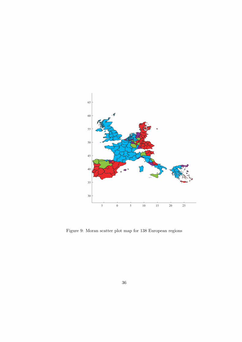
An illustration of the map produced by the function is provided in fig-ure 9 and the associated scatter plot in figure 10. This was constructed usingper capita income growth rates for a sample of 138 European Union regions.There is a great deal of literature that points to a core versus peripherypattern of growth, with regions on the periphery exhibiting high growthwhile those at the core have low growth (Le Gallo, Ertur, and Baumont(2003) and Le Gallo and Ertur (2003)). The color-coding of the map makesthis pattern quite evidence. Cyan-colored core regions occupy the center ofthe map, reflecting low growth for these regions and their neighbors. Red-colored regions represent those where the regions and their neighbors exhibithigh growth rates, which are located on the periphery.
3.3 The arc sarmap function
This function illustrates the benefit from having access to mapping func-tions in a spatial econometric software environment. Fast and efficient spa-tial econometric estimation functions exist for estimating a class of spatialregression models described in Anselin (1988), shown in (3).
y = ρWy + Xβ + u (3)u = λDu + ε, ε ∼ N(0, σ2
εIn)
The terms W and D represent n by n row standardized spatial weightmatrices discussed previously. The n by k matrix X contains k explanatoryvariables, and the dependent variable is y. The parameters to be estimatedare: β, ρ, λ, and σ2
ε . Anselin (1988) notes that a family of models can bederived by: setting the parameter ρ on the spatially lagged dependent vari-able Wy to zero producing a model we label the spatial error model (SEM);setting the parameter λ on the spatially lagged disturbance term to zeroproduces a model we label the spatial autoregressive model (SAR); and a
20

third model can be based on both ρ and λ non-zero, which we label SAC. Yetanother model arises if we introduce spatial lags of the explanatory variablestaking the form WX, along with an associated parameter vector, known asa spatial Durbin model (SDM).
The same functionality of the arc sarmap function that allows the userto explore spatial stability of the SAR model could be provided for theseother models. This could be achieved easily by relying on the fast maximumlikelihood estimation functions from the spatial econometrics toolbox.
In addition to maximum likelihood estimation procedures, algorithms ex-ist for robust Bayesian estimates for this family of models that allow for non-constant variance across the observations. Using Markov Chain Monte Carlo(MCMC) estimation, variance scalar estimates can be produced for each ob-servation using methods described by Geweke (1993) for the case of linearleast-squares and LeSage (1997) for this family of spatial regression models.The ability to plot the variance estimates for each region/observation on amap would help identify regions where the model may be inadequate. Forexample, if urban regions exhibit higher noise variances, this may be anindication of an inadequately modeled regression relationship.
Other approaches to exploring spatial stability that have been proposedare geographically weighted regression (Brunsdon et. al) and Bayesian vari-ants (LeSage, 2004). These models produce locally linear non-parametric es-timates for each observation, based on a sub-sample of observations nearby.Mapping these parameter estimates can be useful in exploring systematicpatterns between the dependent and explanatory variables over space. Paceand LeSage (2004) suggest a spatial autoregressive locally linear estimationprocedure they label SALE, that relies on a recursive estimation schemeto produce estimates for the SAR model for every observation. We useparameter estimates from this model constructed using a function from theSpatial Statistics Toolbox to demonstrate the value of mapping locally linearparameter estimates.
A model from Pace and Barry (1997) of the relationship between voterparticipation in the 1980 presidential election and variables measuring pop-ulation eligible to vote, home ownership, educational attainment and percapita income was estimated using 3,107 observations and the SALE method-ology. This produces 3,107 parameter estimates for each explanatory vari-able in the model. Figure 11 shows the map and legend figures for theestimates of the ‘home ownership’ variable in the model. The histogramlegend shows that this variable exerts a predominately positive impact onvoter participation rates. From the map we see that home ownership exertsa larger impact on voter participation in the south and midwest counties,
21

and a smaller impact for counties on the east and west coasts.
4 Using the Arc Mat Toolbox functions
In this section we discuss issues that arise in using the mapping functions.One is the need to sort spatial econometric data sets to match the orderof the polygon and data information read from the shape files. Anotherissue that arises is the need to construct spatial weight matrices, whichrequire polygon centroids, distances or other features related to the polygonrelationships. These two issues are discussed in the next subsections.
4.1 Merging data for mapping in Matlab
One approach to using the Arc Mat toolbox would be to rely on ArcViewshape files for the mapping polygons and perhaps centroids of the polygons,while relying on a separate data file for spatial econometric analysis. Thisrequires that a geography key be included in the econometric analysis dataset. It is likely such a code would exist in any spatial econometric sampledata. For example, consider a sample of 1,008 Ohio zip code areas and a setof shape files that contain the polygon information as well as the latitudeand longitude centroids for the zip code areas.
An example of the Matlab code needed to sort the spatial econometricdata sample into an order consistent with the polygon ordering in the shapefile is provided below. In this example the shape files are named ‘ohio.dbf’and ‘ohio.shp’, while the spatial econometric data file is named ’odata.txt’.We assume that the zip code identifier is contained in the first column ofthe results.data structure variable matrix obtained from the database file.We also assume that a zip code identifier exists in the first column of thedata file ‘odata.txt’.
22

filename = ‘ohio’;results = shape_read(filename);nobs = results.npoly; % should equal 1,008 the # of observationsmap_zips = results.data(:,1);load odata.txt;dat_zips = odata(:,1);% loop over the map_zips and find an index corresponding to% each of these zip codes in the odata matrixout = zeros(size(odata)); % allocate a matrix for the resultsmissing = zeros(nobs,1); % keep track of missing valuesfor i=1:nobszipi = map_zips(i,1);ind = find(zipi == dat_zips);
if length(ind) > 0out(i,:) = odata(ind,:);
elsemissing(i,1) = 1;
end;end;options.missing = missing;arc_histmap(out,results,options);
The code loops over all zip code areas using the order from the shapefiles. Each zip code area is extracted into the scalar variable ‘zipi’, and thisis used in the Matlab find function that searches the vector ‘dat zips’ for amatching zip code. If a match is found, an index into the vector ‘dat zips’is returned and this index is used to extract a row from the matrix ‘odata’and place it in the matrix ‘out’. If no match is found, we record this in avector ‘missing’ that could be used as an input option to the mapping GUIfunction. Note that in this case the matrix ‘out’ would contain a row ofzero values used to intialize this matrix. This would adversely affect thehistogram legend in the arc histmap function which would interpret theseas actual values without the optional ‘options.missing’ vector used as aninput to the function.
We note that any data information contained in the structure variable‘results.data’ could be combined with the sorted version of the spatial econo-metric sample data matrix. Because these are now sorted by zip code area,Matlab would combine these two matrices with the simple command:
combined = [results.data out];
23

Since regression estimates are unaffected by the ordering of the observa-tions, it would seem that sorting the spatial econometric data to match theorder of the shape file information should occur at the outset. This wouldallow users to map residuals, predicted values and other information using‘results’ structure information returned by the estimation functions in theSpatial Econometrics Toolbox.
4.2 Polygons and spatial weight matrices
Current functions for constructing spatial weight matrices rely on two vec-tors of polygon centroid coordinates. Functions to produce weight matricesbased on contiguity, nearest neighbors and distances using the centroid coor-dinates are part of the Spatial Econometrics and Spatial Statistics Toolboxes.
Centroids of the polygons are returned in the ‘results’ structure of theshape read function. These are constructed using a c/c++ language APIfunction that is part of the public domain shapelib. The function returns thefollowing information regarding latitude and longitude coordinates associ-ated with the polygons, as well as the vectors required to draw the polygons.
results.xmin = an nobs-vector of minimum longitude for each region
results.xmax = an nobs-vector of maximum longitude for each region
results.ymin = an nobs-vector of minimum latitude for each region
results.ymax = an nobs-vector of maximum latitude for each region
results.xc = an nobs-vector with x-centroid for each polygon/region
results.yc = an nobs-vector with y-centroid for each polygon/region
The toolbox functions rely on a Delaunay triangularization scheme tofind neighboring observations, and a Matlab function exists to calculateDelaunay triangles. To illustrate this approach, figure 12 shows a Delaunaytriangularization centered on an observation located at point A. The spaceis partitioned into triangles such that there are no points in the interiorof the circumscribed circle of any triangle. Neighbors could be specifiedusing Delaunay contiguity defined as two points being a vertex of the sametriangle. The neighboring observations to point A that could be used toconstruct a spatial weight matrix are B,C, E, F .
One way to specify a spatial weight matrix W would be to set columnelements associated with neighboring observations B, C,E, F equal to 1 in
24

row A. This would reflect that these observations are neighbors to obser-vation A. Typically, the weight matrix is standardized so that row sumsequal unity, producing a row-stochastic weight matrix. Row-stochastic spa-tial weight matrices, or multidimensional linear filters, have a long historyof application in spatial statistics (e.g., Ord, 1975).
An alternative approach would be to rely on neighbors ranked by dis-tance from observation A. We can simply compute the distance from A toall other observations and rank these by size. In the case of figure 1 wewould have: a nearest neighbor E, the nearest 2 neighbors E, C, nearest3 neighbors E, C,D, and so on. Again, we could set elements WAj = 1for observations j in row A to reflect any number of nearest neighbors toobservation A, and transform to row-stochastic form. This approach mightinvolve including a determination of the appropriate number of neighborsas part of the model estimation problem.
Weight matrices can be constructed using functions: xy2cont and make nnw,which produce contiguity and nearest neighbor weight matrices respectively.Their usage takes the form:
[W1,W2,W3] = xy2cont(latitude,longitude);Wm = make_nnw(latitude,longitude,m);
The function xy2cont returns three sparse weight matrices:
W1 = W*S*W, a symmetric spatial weight matrix with maximumeigenvalue equal to one, and the matrix S represents the adjacencymatrix with Delaunay triangles based on a Voronoi tesselation.
W2 = W*W*S, a row-stochastic spatial weight matrix,
W3 = diagonal matrix with diagonal elements equal to the inverse ofthe row sums.
while the function make nnw returns a row-stochastic sparse weight matrixbased on the m nearest neighbors.
The polygon coordinates produced by extracting information from theArcView shape files should allow additional weight matrix functions. Forexample, weight matrices that rely on the relative length of common bordersbetween two regions could be constructed. Shape files containing informa-tion concerning highway linkages and other geographical features from themap of regions could in theory also be used to provide information for usein constructing weight matrices for use in spatial analysis. This remains atopic for future exploration.
25

There is also the potential to use polygon boundaries along with the data-base information to identify map zones that correspond to abrupt change invariables of interest, a process known as wombling, after a seminal paper onthis topic by Womble (1951). This is a popular technique used by amongothers, geneticists, demographers, and environmental scientists in spatialstatistical work. The goal of these methods is to identify important regionaldifferences across shared borders of the regions of analysis that might relateto “barriers” or “edge detection”. For example, wombling analysis was usedby Bocquet-Appel and Jakobi (1996) to identify barriers in population diffu-sion that impacted the demographic transition in Europe. Recent womblingwork for point level data rather than areal data (where information is ag-gregated or averaged over geopolitical regions) by Banerjee, Gelfand, andSirmans (2004) relies on Bayesian hierarchical spatial statistical models todetermine boundaries by locating points associated with abrupt gradientchanges measured on a fitted spatial surface. The ability to extract mappolygon information into a spatial statistical software environment shouldadvance research on wombling. For this type of modeling, the need for inter-active visualization of polygon boundaries based on statistical classificationcalculations remains a key to this type of analysis. Existing software suchas BoundaySeer Maruca, and Jacquez (2002) provides some functionalityalong these lines but lacks the capability to implement Bayesian hierarchi-cal models and Markov Chain Monte Carlo estimation methods.
5 Conclusions
The ability to the use statistical functionality for spatial modeling and analy-sis in conjunction with a mapping interface in the same environment hasreceived a great deal of attention in the spatial analysis literature, datingat least to Anselin (1994). We demonstrate the feasibility of extractingmap polygon and database information from ArcView shape files for use instatistical software environments. The motivation for extracting databaseinformation for use in a statistical programming environment seems quiteevident. We demonstrate that information containing map polygons canalso be used in these environments to produce high quality mapping func-tionality. Improvements in recent computer graphics hardware and softwarehave arisen from interest in computer gaming. This allows rapid renderingof map polygons on almost all recent desktop and laptop computers usingbasic plotting functionality that is part of statistical software environments.A byproduct of this is that mapping functionality based on the high quality
26

ArcView map polygons can be created in a statistical software environmentin support of spatial econometric and statistical analysis. Although ourfocus was on a particular implementation of these ideas in the Matlab soft-ware environment, a similar approach would be feasible in a number of otherstatistical software environments such as R/Splus, Octave and SciLab.
Polygon information extracted from ArcView shape files can also be usedin conjunction with the GeoXP Toolbox of public domain programs for link-ing spatial statistics in both Matlab and R/Splus software environments.These functions have been constructed to take advantage of polygon coordi-nates, but no facility for importing this information into Matlab or R/Splusenvironments is provided in the toolbox. Polygon plotting in GeoXP takesthe form of line plots not filled polygons which makes the task of visual-ization slightly more difficult. One area for future development would beadditional GUI mapping functions along the lines of the extensive set offunctionality contained in GeoXP.
Another avenue for future development of the Arc Mat Toolbox mightinclude the ability to produce shape files as output. These might contain al-tered information based on spatial statistical analysis, for example womblingmethods. Since this type of spatial analysis leads to creation of new spatialconnectivity or linkage structures, the ability to write this information tonew shape files would be valuable.
27
6 References
Anselin L. (1988), Spatial Econometrics: Methods and Models, KluwerAcademic Publishers, Dordrecht.
Anselin, L. (1994), “Exploratory Spatial Data Analysis and GeographicInformation Systems,” in M. Painho (ed.), New Tools for Spatial Analy-sis, Eurostat, Luxembourg, 1994, pp. 4554.
Luc Anselin, Ibnu Syabri and Oleg Smirnov (2002), “Visualizing Mul-tivariate Spatial Correlation with Dynamically Linked Windows,” InL. Anselin and S. Rey (Eds.), Proceedings, CSISS Workshop on NewTools for Spatial Data Analysis, Santa Barbara, CA, May 10-11, 2002.Center for Spatially Integrated Social Science, CD-ROM (pdf file,20pp, 517K).
Banerjee, S., A.E. Gelfand and C.F. Sirmans (2004) “Directional ratesof change under spatial process models,” Journal of the American Sta-tistical Association, Vol. 98, pp. 946-954.
Anselin, Luc and Shuming Bao. 1997. “Exploratory Spatial DataAnalysis Linking SpaceStat and ArcView,” In: Manfred Fischer andArthur Getis (Eds.), Recent Developments in Spatial Analysis, Berlin:Springer-Verlag, pp35-59.
Barry R., Pace R.K. (1999), ”A Monte Carlo Estimator of the LogDeterminant of Large Sparse Matrices”, Linear Algebra and its Appli-cations, Vol. 289, pp. 41-54.
Bivand, Roger S. (2002) “Spatial econometrics functions in R: Classesand methods”, Journal of Geographical Systems, Vol. 4, pp. 405-421.
Bocquet-Appel, J.P., and L. Jakobi. (1996) “Barriers for the spatialdiffusion for the demographic transition in Europe,” in Spatial Analysisof Biodemographic Data, J.P. Bocquet-Appel, D. Courgeau and D.Pumain (eds.) Eurotext, John Libbey, London and Paris.
Brunsdon, C., A. S. Fotheringham, and M.E. Charlton (1996), “Geo-graphically weighted regression: A method for exploring spatial non-stationarity,” Geographical Analysis, Vol. 28, pp. 281-298.
Geweke J. (1993), “Bayesian Treatment of the Independent Student tLinear Model,” Journal of Applied Econometrics, Vol. 8, pp. 19-40.
28

Goodchild, Michael F. and Robert Haining (2003), “GIS and spatialdata analysis: Converging perspectives,” Papers in Regional Science,Vol. 83, pp. 363-385.
Heba, Ines, Eric Malin and Christine Thomas-Agnan, (2002) “Ex-ploratory spatial data analysis with GEOXP,” European Regional Sci-ence Association conference papers.
Le Gallo, J., C. Ertur C., Baumont C. (2003) “A Spatial Economet-ric Analysis of Convergence across European Regions, 1980-1995,” inEuropean Regional Growth, B. Fingleton, (ed.), Springer-Verlag, Ad-vances in Spatial Science, pp. 99-130.
Le Gallo J., and C. Ertur (2003) “Exploratory spatial data analysisof the distribution of regional per capita GDP in Europe, 1980-1995,”Papers in Regional Science, Vol. 82 no. 2, pp. 175-201.
LeSage, James P. (1997) “Bayesian Estimation of Spatial Autoregres-sive Models,” International Regional Science Review, Vol. 20, nos.1&2, pp. 113-129.
LeSage, J.P. (2004) “A Family of Geographically Weighted Regres-sion Models,” forthcoming in Advances in Spatial Econometrics, LucAnselin, J.G.M. Florax and S.J. Rey (eds.) Springer-Verlag.
Maruca, S.L., and G.M. Jacquez. (2002) “Area-based tests for associ-ation between spatial patterns,” Journal of Geographic Systems Vol.4 no. 1, pp. 69-83.
Ord, J.K. (1975), “Estimation Methods for Models of Spatial Inter-action,” Journal of the American Statistical Association, Vol. 70, pp.120-126.
Pace, R. Kelley, and Ronald Barry, “Quick Computation of Regres-sions with a Spatially Autoregressive Dependent Variable,” Geograph-ical Analysis, 29, 3, 1997, 232-247.
Pace, R.K, LeSage. James P., (2004) “Spatial Autoregressive LocalEstimation,” in Recent Advances in Spatial Econometrics, Jesus Mur,Henri Zoller and Arthur Getis (eds.), Palgrave Publishers, pp. 31-51.
Womble, W. (1951) “Differential systematics,” Science, Vol. 114, pp.315-322.
29

3 2.5 2 1.5 1 0.5 0 0.5 1 1.5 2
x 106
�0.5
0
0.5
1
1.5
2
2.5
3
3.5
4
4.5
x 106
Figure 1: China map of population growth rates 1980-1995
0.1 0.15 0.2 0.25 0.3 0.35 0.40
2
4
6
8
10
12
pop growth 80-95
Figure 2: Legend for China map of population growth rates
30

−0.1 −0.05 0 0.05 0.1 0.15
−0.06
−0.04
−0.02
0
0.02
0.04
1
2
3
4
5
6
7
8
910
11
12
13
14
15
16
17
18 1920
21
22
23
24
25
26
27
28
29
30
population growth
W*p
opul
atio
n gr
owth
Figure 3: Moran scatter plot for Chinese provincial population growth rates
3 2.5 2 1.5 1 0.5 0 0.5 1 1.5 2
x 106
�0.5
0
0.5
1
1.5
2
2.5
3
3.5
4
4.5
x 106
1
23
4
5
6
7
8
9
10
11
12
13
14
15
16
17
18
1920
21
22
23
24
25
26
27
2829
30
Figure 4: China map linked to the moran scatter plot
31

1.3 1.2 1.1 1 0.9 0.8
x 107
2
3
4
5
6
7
x 106
Figure 5: SAR model selection map
32

Figure 6: SAR model comparison of global and sub-sample estimates
33

Figure 7: A screen showing the arc histmap GUI
34

20 30 40 50 60 70 80 90 1000
0.5
1
1.5
2
2.5
3
3.5
4
4.5
5
4th grade citizenship
Figure 8: Histogram with linked map zoomed in on Toledo, Ohio
35
5 0 5 10 15 20 25
30
35
40
45
50
55
60
65
Figure 9: Moran scatter plot map for 138 European regions
36

0.05 0 0.05 0.1
0.02
0.01
0
0.01
0.02
0.03
0.04
0.05
0.06
0.07
0.08
per capita income growth
W*p
er c
apit
a in
com
e g
row
th
Figure 10: Moran scatter plot for European Union regions
37

Figure 11: SALE parameter estimates for the home ownership variable
38

0 1 2 3 4 5 6 7 8
0
1
2
3
4
5
A
B
C
D
E
F
G
X-Coordinates
Y-Coordinates
Figure 12: Delaunay triangularization
39