lecture 2: over tting. regularization · lecture 2: over tting. regularization generalizing...

Lecture 2: Overfitting. Regularization

• Generalizing regression

• Overfitting

• Cross-validation

• L2 and L1 regularization for linear estimators

• A Bayesian interpretation of regularization

• Bias-variance trade-off

COMP-652 and ECSE-608, Lecture 2 - January 10, 2017 1

Recall: Overfitting

• A general, HUGELY IMPORTANT problem for all machine learningalgorithms

• We can find a hypothesis that predicts perfectly the training data butdoes not generalize well to new data

• E.g., a lookup table!


Another overfitting example

x

t

M = 0

0 1

−1

0

1

x

t

M = 1

0 1

−1

0

1

x

t

M = 3

0 1

−1

0

1

x

t

M = 9

0 1

−1

0

1

• The higher the degree of the polynomial M , the more degrees of freedom,and the more capacity to “overfit” the training data

• Typical overfitting means that error on the training data is very low, buterror on new instances is high


Overfitting more formally

• Assume that the data is drawn from some fixed, unknown probabilitydistribution

• Every hypothesis has a ”true” error J∗(h), which is the expected errorwhen data is drawn from the distribution.

• Because we do not have all the data, we measure the error on the trainingset JD(h)

• Suppose we compare hypotheses h1 and h2 on the training set, andJD(h1) < JD(h2)

• If h2 is ”truly” better, i.e. J∗(h2) < J∗(h1), our algorithm is overfitting.

• We need theoretical and empirical methods to guard against it!


Typical overfitting plot

M

ERMS

0 3 6 90

0.5

1TrainingTest

• The training error decreases with the degree of the polynomial M , i.e.the complexity of the hypothesis• The testing error, measured on independent data, decreases at first, then

starts increasing• Cross-validation helps us:

– Find a good hypothesis class (M in our case), using a validation setof data

– Report unbiased results, using a test set, untouched during eitherparameter training or validation


Cross-validation

• A general procedure for estimating the true error of a predictor

• The data is split into two subsets:

– A training and validation set used only to find the right predictor– A test set used to report the prediction error of the algorithm

• These sets must be disjoint!

• The process is repeated several times, and the results are averaged toprovide error estimates.


Example: Polynomial regression

x

y

x

y

x

y

x

y


Leave-one-out cross-validation

1. For each order of polynomial, d:

(a) Repeat the following procedure m times:i. Leave out ith instance from the training set, to estimate the true

prediction error; we will put it in a validation setii. Use all the other instances to find best parameter vector, wd,i

iii. Measure the error in predicting the label on the instance left out,for the wd,i parameter vector; call this Jd,i

iv. This is a (mostly) unbiased estimate of the true prediction error(b) Compute the average of the estimated errors: Jd = 1

m

∑mi=1 Jd,i

2. Choose the d with lowest average estimated error: d∗ = arg mind J(d)


Estimating true error for d = 1

D = {(0.86, 2.49), (0.09, 0.83), (−0.85,−0.25), (0.87, 3.10), (−0.44, 0.87),(−0.43, 0.02), (−1.10,−0.12), (0.40, 1.81), (−0.96,−0.83), (0.17, 0.43)}.

Iter Dtrain Dvalid Errortrain Errorvalid (J1,i)1 D − {(0.86, 2.49)} (0.86, 2.49) 0.4928 0.00442 D − {(0.08, 0.83)} (0.09, 0.83) 0.1995 0.18693 D − {(−0.85,−0.25)} (−0.85,−0.25) 0.3461 0.00534 D − {(0.87, 3.10)} (0.87, 3.10) 0.3887 0.86815 D − {(−0.44, 0.87)} (−0.44, 0.87) 0.2128 0.34396 D − {(−0.43, 0.02)} (−0.43, 0.02) 0.1996 0.15677 D − {(−1.10,−0.12)} (−1.10,−0.12) 0.5707 0.72058 D − {(0.40, 1.81)} (0.40, 1.81) 0.2661 0.02039 D − {(−0.96,−0.83)} (−0.96,−0.83) 0.3604 0.2033

10 D − {(0.17, 0.43)} (0.17, 0.43) 0.2138 1.0490mean: 0.2188 0.3558


Leave-one-out cross-validation results

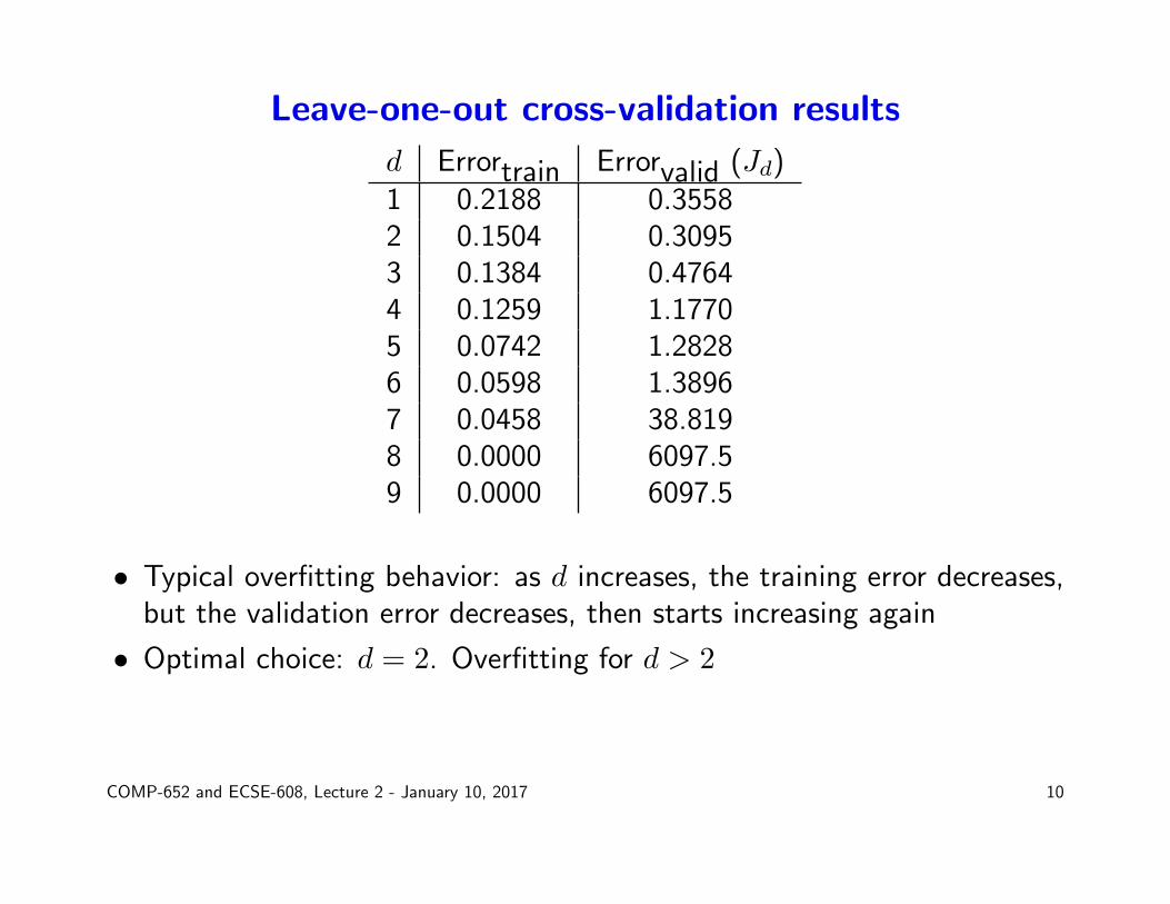
d Errortrain Errorvalid (Jd)1 0.2188 0.35582 0.1504 0.30953 0.1384 0.47644 0.1259 1.17705 0.0742 1.28286 0.0598 1.38967 0.0458 38.8198 0.0000 6097.59 0.0000 6097.5

• Typical overfitting behavior: as d increases, the training error decreases,but the validation error decreases, then starts increasing again

• Optimal choice: d = 2. Overfitting for d > 2


Estimating both hypothesis class and true error

• Suppose we want to compare polynomial regression with some otheralgorithm

• We chose the hypothesis class (i.e. the degree of the polynomial, d∗)based on the estimates Jd

• Hence Jd∗ is not unbiased - our procedure was aimed at optimizing it

• If we want to have both a hypothesis class and an unbiased error estimate,we need to tweak the leave-one-out procedure a bit


Cross-validation with validation and testing sets

1. For each example j:

(a) Create a test set consisting just of the jth example, Dj = {(xj, yj)}and a training and validation set D̄j = D − {(xj, yj)}

(b) Use the leave-one-out procedure from above on Dj (once!) to find ahypothesis, h∗j• Note that this will split the data internally, in order to both train

and validate!• Typically, only one such split is used, rather than all possible splits

(c) Evaluate the error of h∗j on Dj (call it J(h∗j))2. Report the average of the J(h∗j), as a measure of performance of the

whole algorithm

• Note that at this point we do not have one predictor, but several!• Several methods can then be used to come up with just one predictor

(more on this later)


Summary of leave-one-out cross-validation

• A very easy to implement algorithm

• Provides a great estimate of the true error of a predictor

• It can indicate problematic examples in a data set (when using multiplealgorithms)

• Computational cost scales with the number of instances (examples), soit can be prohibitive, especially if finding the best predictor is expensive

• We do not obtain one predictor, but many!

• Alternative: k-fold cross-validation: split the data set into k parts, thenproceed as above.


Regularization

• Remember the intuition: complicated hypotheses lead to overfitting

• Idea: change the error function to penalize hypothesis complexity:

J(w) = JD(w) + λJpen(w)

This is called regularization in machine learning and shrinkage in statistics

• λ is called regularization coefficient and controls how much we valuefitting the data well, vs. a simple hypothesis


Regularization for linear models

• A squared penalty on the weights would make the math work nicely inour case:

1

2(Φw − y)T (Φw − y) +

λ

2wTw

• This is also known as L2 regularization, or weight decay in neuralnetworks

• By re-grouping terms, we get:

JD(w) =1

2(wT (ΦTΦ + λI)w −wTΦTy − yTΦw + yTy)

• Optimal solution (obtained by solving ∇wJD(w) = 0)

w = (ΦTΦ + λI)−1ΦTy


What L2 regularization does

arg minw

1

2(Φw − y)T (Φw − y) +

λ

2wTw = (ΦTΦ + λI)−1ΦTy

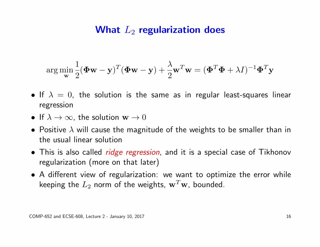
• If λ = 0, the solution is the same as in regular least-squares linearregression

• If λ→∞, the solution w→ 0

• Positive λ will cause the magnitude of the weights to be smaller than inthe usual linear solution

• This is also called ridge regression, and it is a special case of Tikhonovregularization (more on that later)

• A different view of regularization: we want to optimize the error whilekeeping the L2 norm of the weights, wTw, bounded.


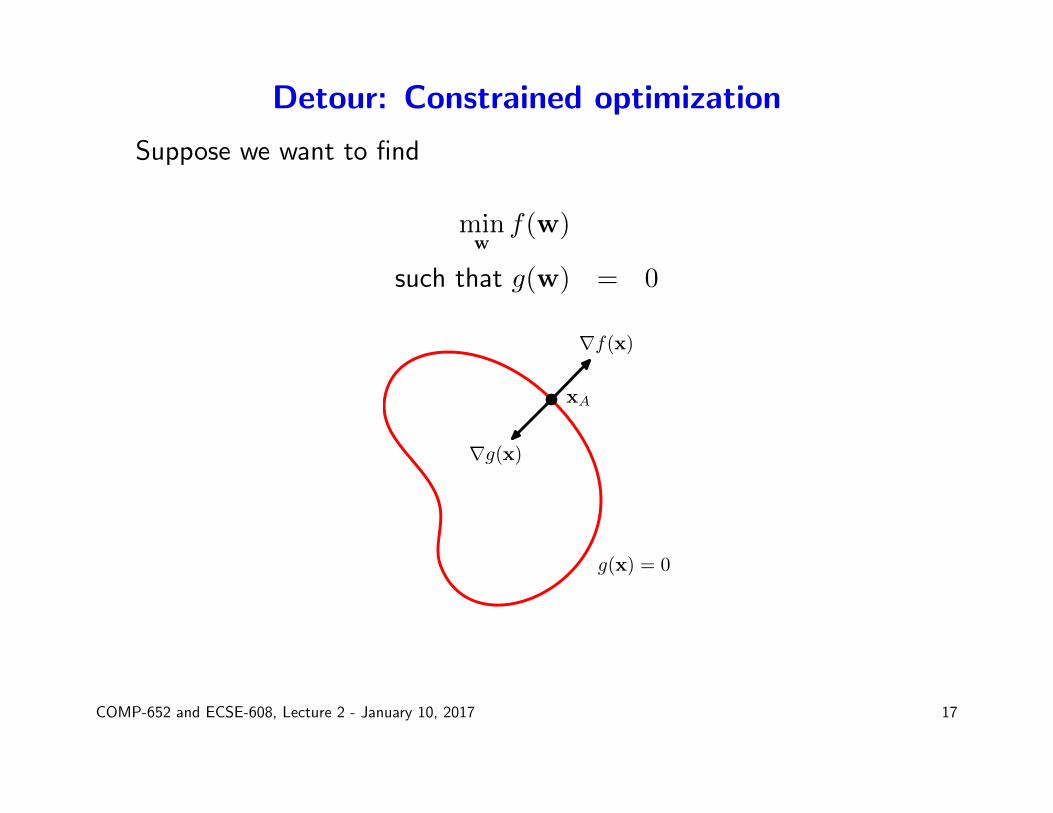
Detour: Constrained optimization

Suppose we want to find

minwf(w)

such that g(w) = 0

∇f(x)

∇g(x)

xA

g(x) = 0


Detour: Lagrange multipliers

∇f(x)

∇g(x)

xA

g(x) = 0

• ∇g has to be orthogonal to the constraint surface (red curve)

• At the optimum, ∇f and ∇g have to be parallel (in same or oppositedirection)

• Hence, there must exist some λ ∈ R such that ∇f + λ∇g = 0

• Lagrangian function: L(x, λ) = f(x) + λg(x)λ is called Lagrange multiplier

• We obtain the solution to our optimization problem by setting both∇xL = 0 and ∂L

∂λ = 0


Detour: Inequality constraints

• Suppose we want to find

minwf(w)

such that g(w) ≥ 0

∇f(x)

∇g(x)

xA

xB

g(x) = 0g(x) > 0

• In the interior (g(x > 0)) - simply find ∇f(x) = 0

• On the boundary (g(x = 0)) - same situation as before, but the signmatters this timeFor minimization, we want ∇f pointing in the same direction as ∇g


Detour: KKT conditions

• Based on the previous observations, let the Lagrangian be L(x, λ) =f(x)− λg(x)

• We minimize L wrt x subject to the following constraints:

λ ≥ 0

g(x) ≥ 0

λg(x) = 0

• These are called Karush-Kuhn-Tucker (KKT) conditions


L2 Regularization for linear models revisited

• Optimization problem: minimize error while keeping norm of the weightsbounded

minwJD(w) = min

w(Φw − y)T (Φw − y)

such that wTw ≤ η

• The Lagrangian is:

L(w, λ) = JD(w)−λ(η−wTw) = (Φw−y)T (Φw−y) +λwTw−λη

• For a fixed λ, and η = λ−1, the best w is the same as obtained byweight decay


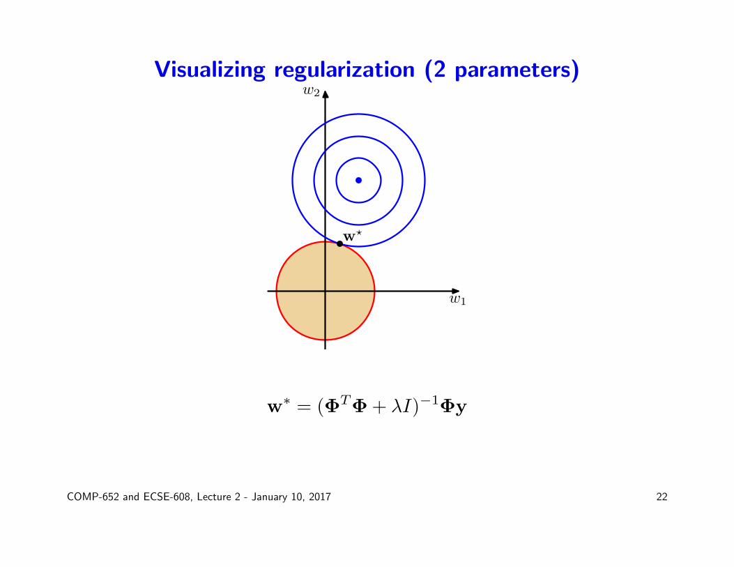
Visualizing regularization (2 parameters)

w1

w2

w?

w∗ = (ΦTΦ + λI)−1Φy


Pros and cons of L2 regularization

• If λ is at a “good” value, regularization helps to avoid overfitting

• Choosing λ may be hard: cross-validation is often used

• If there are irrelevant features in the input (i.e. features that do notaffect the output), L2 will give them small, but non-zero weights.

• Ideally, irrelevant input should have weights exactly equal to 0.


L1 Regularization for linear models

• Instead of requiring the L2 norm of the weight vector to be bounded,make the requirement on the L1 norm:

minwJD(w) = min

w(Φw − y)T (Φw − y)

such thatn∑i=1

|wi| ≤ η

• This yields an algorithm called Lasso (Tibshirani, 1996)


Solving L1 regularization

• The optimization problem is a quadratic program

• There is one constraint for each possible sign of the weights (2n

constraints for n weights)

• For example, with two weights:

minw1,w2

m∑j=1

(yj − w1x1 − w2x2)2

such that w1 + w2 ≤ η

w1 − w2 ≤ η

−w1 + w2 ≤ η

−w1 − w2 ≤ η

• Solving this program directly can be done for problems with a smallnumber of inputs


Visualizing L1 regularization

w1

w2

w?

• If λ is big enough, the circle is very likely to intersect the diamond atone of the corners

• This makes L1 regularization much more likely to make some weightsexactly 0


Pros and cons of L1 regularization

• If there are irrelevant input features, Lasso is likely to make their weights0, while L2 is likely to just make all weights small

• Lasso is biased towards providing sparse solutions in general

• Lasso optimization is computationally more expensive than L2

• More efficient solution methods have to be used for large numbers ofinputs (e.g. least-angle regression, 2003).

• L1 methods of various types are very popular


Example of L1 vs L2 effect

Example: lasso vs. ridge

From HTF: prostate dataRed lines: choice of � by 10-fold CV.

Degrees of Freedom

Coe

ffici

ents

0 2 4 6 8

-0.2

0.0

0.2

0.4

0.6

•

••••••

••

••

••

••

••

••

•••••

•

lcavol

••••••••••••••••••••••••

•

lweight

•••••••••••••••••••••••••

age

•••••••••••••••••••••••••

lbph

••••••••••••••••••••••••

•

svi

•

•••••

••

••

•••••••••••••••

lcp

••••••••••••••••••••••••

•gleason

••••••••••••••••••••••••

•

pgg45

Shrinkage Factor s

Coe

ffici

ents

0.0 0.2 0.4 0.6 0.8 1.0

-0.2

0.0

0.2

0.4

0.6

•

•

•

•

•

••

• • • • • • • • • • • • • • • • • • lcavol

• • • • ••

••

•• • • • • • • • • • • • • • • • lweight

• • • • • • • • • • • • • • • • • • • • • • • • •age

• • • • • • • • • ••

••

•• • • • • • • • • • • lbph

• • • • • • ••

••

••

•• • • • • • • • • • • •svi

• • • • • • • • • • • • • • • ••

••

••

••

•• lcp

• • • • • • • • • • • • • • • • • • • • • • • • •gleason• • • • • • • • • • • • • • • • • • • • • • • ••pgg45

CS195-5 2006 – Lecture 14 7

• Note the sparsity in the coefficients induces by L1

• Lasso is an efficient way of performing the L1 optimization


Bayesian view of regularization

• Start with a prior distribution over hypotheses

• As data comes in, compute a posterior distribution

• We often work with conjugate priors, which means that when combiningthe prior with the likelihood of the data, one obtains the posterior in thesame form as the prior

• Regularization can be obtained from particular types of prior (usually,priors that put more probability on simple hypotheses)

• E.g. L2 regularization can be obtained using a circular Gaussian prior forthe weights, and the posterior will also be Gaussian

• E.g. L1 regularization uses double-exponential prior (see (Tibshirani,1996))


Bayesian view of regularization

• Prior is round Gaussian

• Posterior will be skewed by the data


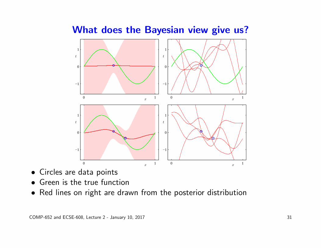
What does the Bayesian view give us?

x

t

0 1

−1

0

1

x

t

0 1

−1

0

1

x

t

0 1

−1

0

1

x

t

0 1

−1

0

1

• Circles are data points• Green is the true function• Red lines on right are drawn from the posterior distribution



x

t

0 1

−1

0

1

x

t

0 1

−1

0

1

x

t

0 1

−1

0

1

x

t

0 1

−1

0

1

• Functions drawn from the posterior can be very different

• Uncertainty decreases where there are data points



• Uncertainty estimates, i.e. how sure we are of the value of the function

• These can be used to guide active learning: ask about inputs for whichthe uncertainty in the value of the function is very high

• In the limit, Bayesian and maximum likelihood learning converge to thesame answer

• In the short term, one needs a good prior to get good estimates of theparameters

• Sometimes the prior is overwhelmed by the data likelihood too early.

• Using the Bayesian approach does NOT eliminate the need to do cross-validation in general

• More on this later...


The anatomy of the error of an estimator

• Suppose we have examples 〈x, y〉 where y = f(x) + ε and ε is Gaussiannoise with zero mean and standard deviation σ• We fit a linear hypothesis h(x) = wTx, such as to minimize sum-squared

error over the training data:

m∑i=1

(yi − h(xi))2

• Because of the hypothesis class that we chose (hypotheses linear inthe parameters) for some target functions f we will have a systematicprediction error• Even if f were truly from the hypothesis class we picked, depending on

the data set we have, the parameters w that we find may be different;this variability due to the specific data set on hand is a different sourceof error


Bias-variance analysis

• Given a new data point x, what is the expected prediction error?• Assume that the data points are drawn independently and identically

distributed (i.i.d.) from a unique underlying probability distributionP (〈x, y〉) = P (x)P (y|x)• The goal of the analysis is to compute, for an arbitrary given point x,

EP[(y − h(x))2|x

]where y is the value of x in a data set, and the expectation is over alltraining sets of a given size, drawn according to P• For a given hypothesis class, we can also compute the true error, which

is the expected error over the input distribution:∑x

EP[(y − h(x))2|x

]P (x)

(if x continuous, sum becomes integral with appropriate conditions).• We will decompose this expectation into three components


Recall: Statistics 101

• Let X be a random variable with possible values xi, i = 1 . . . n and withprobability distribution P (X)

• The expected value or mean of X is:

E[X] =

n∑i=1

xiP (xi)

• If X is continuous, roughly speaking, the sum is replaced by an integral,and the distribution by a density function

• The variance of X is:

V ar[X] = E[(X − E(X))2]

= E[X2]− (E[X])2


The variance lemma

V ar[X] = E[(X − E[X])2]

=

n∑i=1

(xi − E[X])2P (xi)

=

n∑i=1

(x2i − 2xiE[X] + (E[X])2)P (xi)

=

n∑i=1

x2iP (xi)− 2E[X]

n∑i=1

xiP (xi) + (E[X])2n∑i=1

P (xi)

= E[X2]− 2E[X]E[X] + (E[X])2 · 1= E[X2]− (E[X])2

We will use the form:

E[X2] = (E[X])2 + V ar[X]


Bias-variance decomposition

• Simple algebra:

EP[(y − h(x))2|x

]= EP

[(h(x))2 − 2yh(x) + y2|x

]= EP

[(h(x))2|x

]+ EP

[y2|x

]− 2EP [y|x]EP [h(x)|x]

• Let h̄(x) = EP [h(x)|x] denote the mean prediction of the hypothesis atx, when h is trained with data drawn from P

• For the first term, using the variance lemma, we have:

EP [(h(x))2|x] = EP [(h(x)− h̄(x))2|x] + (h̄(x))2

• Note that EP [y|x] = EP [f(x) + ε|x] = f(x) (because of linearity ofexpectation and the assumption on ε ∼ N (0, σ))

• For the second term, using the variance lemma, we have:

E[y2|x] = E[(y − f(x))2|x] + (f(x))2


Bias-variance decomposition (2)

• Putting everything together, we have:

EP[(y − h(x))2|x

]= EP [(h(x)− h̄(x))2|x] + (h̄(x))2 − 2f(x)h̄(x)

+ EP [(y − f(x))2|x] + (f(x))2

= EP [(h(x)− h̄(x))2|x] + (f(x)− h̄(x))2

+ E[(y − f(x))2|x]

• The first term, EP [(h(x) − h̄(x))2|x], is the variance of the hypothesish at x, when trained with finite data sets sampled randomly from P

• The second term, (f(x) − h̄(x))2, is the squared bias (or systematicerror) which is associated with the class of hypotheses we are considering

• The last term, E[(y−f(x))2|x] is the noise, which is due to the problemat hand, and cannot be avoided


Error decomposition

ln λ

−3 −2 −1 0 1 20

0.03

0.06

0.09

0.12

0.15

(bias)2

variance

(bias)2 + variancetest error

• The bias-variance sum approximates well the test error over a set of 1000points

• x-axis measures the hypothesis complexity (decreasing left-to-right)

• Simple hypotheses usually have high bias (bias will be high at manypoints, so it will likely be high for many possible input distributions)

• Complex hypotheses have high variance: the hypothesis is very dependenton the data set on which it was trained.


Bias-variance trade-off

• Typically, bias comes from not having good hypotheses in the consideredclass

• Variance results from the hypothesis class containing “too many”hypotheses

• MLE estimation is typically unbiased, but has high variance

• Bayesian estimation is biased, but typically has lower variance

• Hence, we are faced with a trade-off: choose a more expressive classof hypotheses, which will generate higher variance, or a less expressiveclass, which will generate higher bias

• Making the trade-off has to depend on the amount of data available tofit the parameters (data usually mitigates the variance problem)


More on overfitting

• Overfitting depends on the amount of data, relative to the complexity ofthe hypothesis

• With more data, we can explore more complex hypotheses spaces, andstill find a good solution

x

t

N = 15

0 1

−1

0

1

x

t

N = 100

0 1

−1

0

1


lecture 2: over tting. regularization · lecture 2: over tting. regularization generalizing...

Documents