lecture 2 production, costs, profits - university of...
TRANSCRIPT
Lecture 2Production, Costs, Profits
1
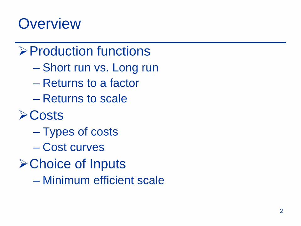
Overview
Production functions– Short run vs. Long run– Returns to a factor– Returns to scale
Costs– Types of costs– Cost curves
Choice of Inputs– Minimum efficient scale
2
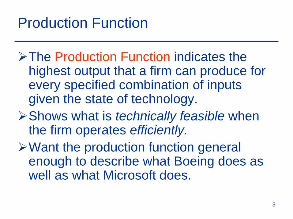
Production Function
The Production Function indicates the highest output that a firm can produce for every specified combination of inputs given the state of technology.Shows what is technically feasible when
the firm operates efficiently.Want the production function general
enough to describe what Boeing does as well as what Microsoft does.
3
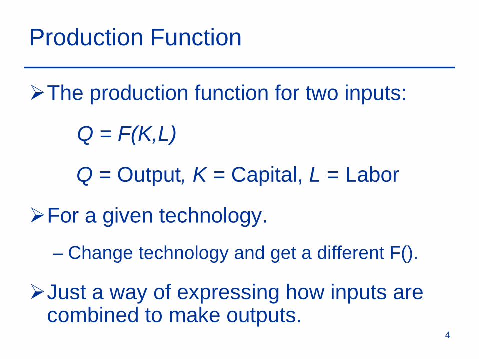
Production Function
The production function for two inputs:
Q = F(K,L)
Q = Output, K = Capital, L = Labor
For a given technology.
– Change technology and get a different F().
Just a way of expressing how inputs are combined to make outputs.
4
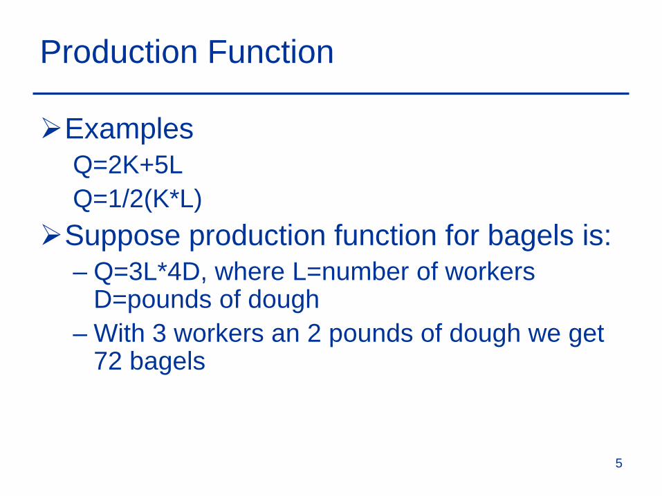
Production Function
ExamplesQ=2K+5LQ=1/2(K*L)
Suppose production function for bagels is: – Q=3L*4D, where L=number of workers
D=pounds of dough– With 3 workers an 2 pounds of dough we get
72 bagels
5
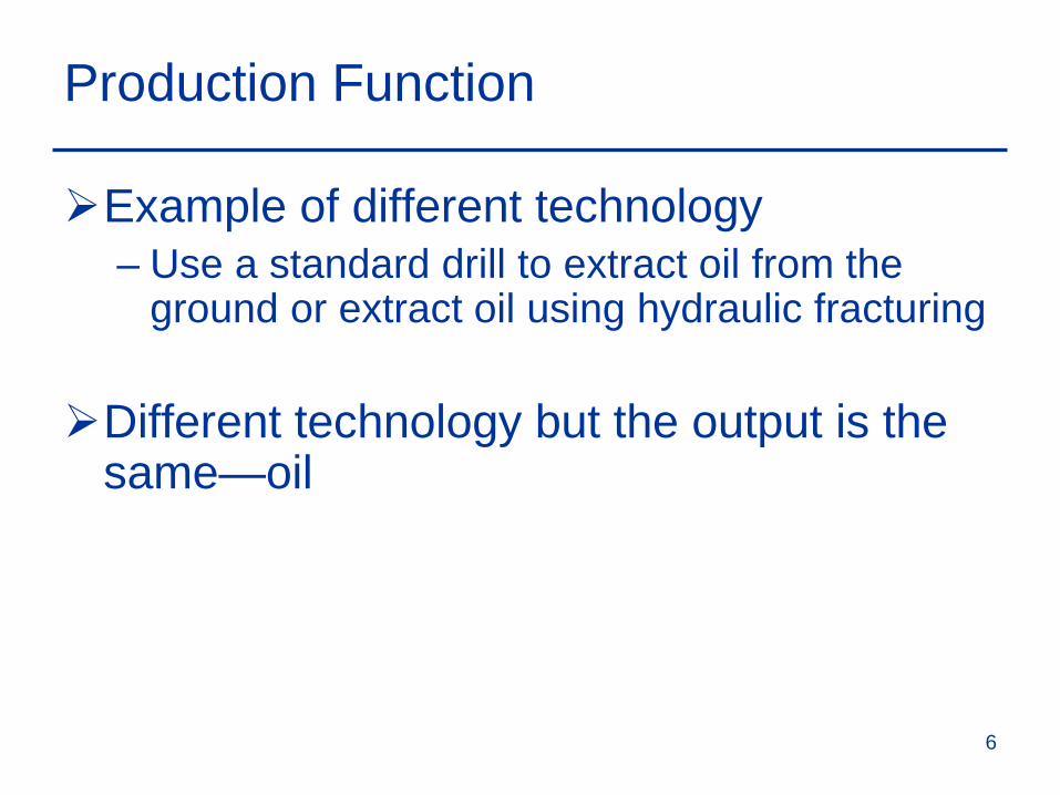
Production Function
Example of different technology– Use a standard drill to extract oil from the
ground or extract oil using hydraulic fracturing
Different technology but the output is the same—oil
6
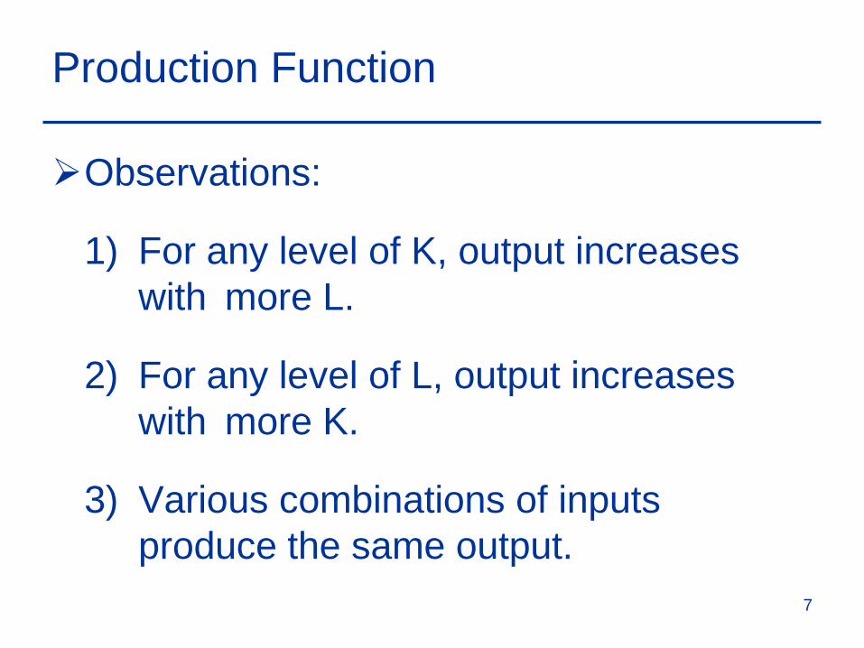
Production Function
Observations:
1) For any level of K, output increases with more L.
2) For any level of L, output increases with more K.
3) Various combinations of inputs produce the same output.
7
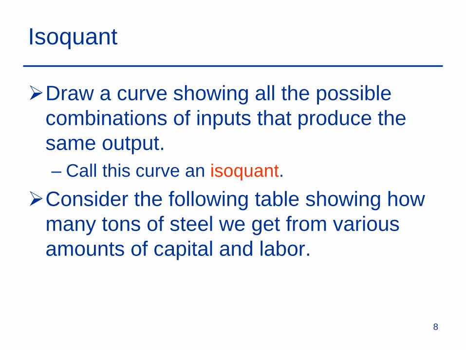
Isoquant
Draw a curve showing all the possible combinations of inputs that produce the same output.– Call this curve an isoquant.
Consider the following table showing how many tons of steel we get from various amounts of capital and labor.
8
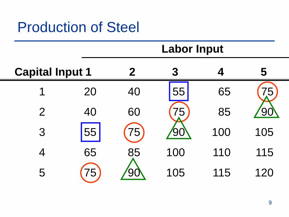
Production of Steel
1 20 40 55 65 75
2 40 60 75 85 90
3 55 75 90 100 105
4 65 85 100 110 115
5 75 90 105 115 120
Capital Input 1 2 3 4 5
Labor Input
9
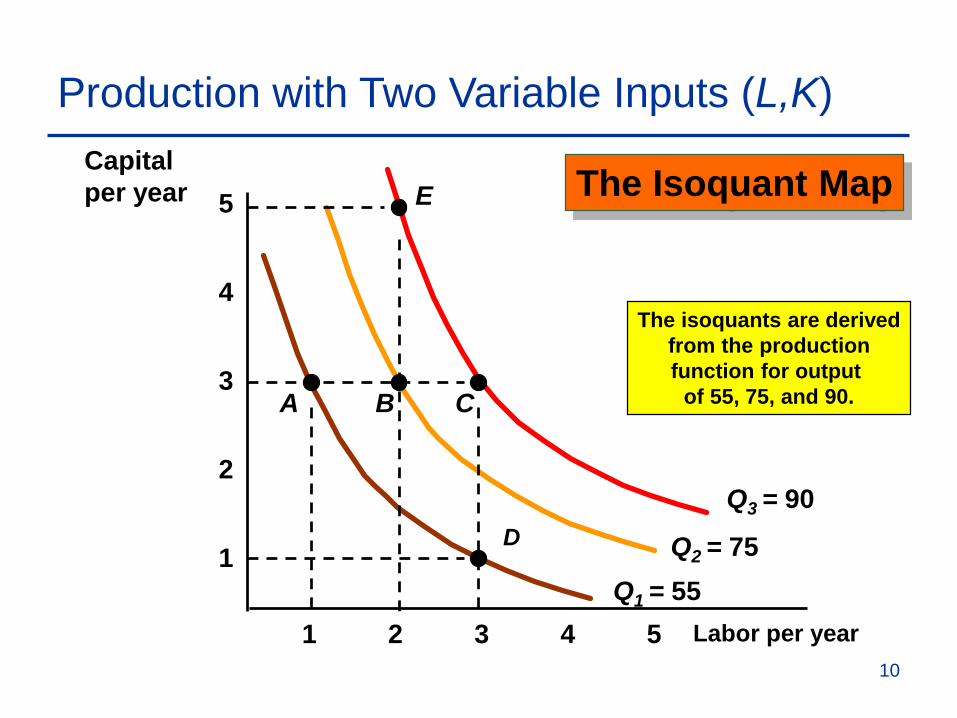
Production with Two Variable Inputs (L,K)
Labor per year
1
2
3
4
1 2 3 4 5
5
Q1 = 55
The isoquants are derivedfrom the productionfunction for output
of 55, 75, and 90.A
D
B
Q2 = 75
Q3 = 90
C
ECapitalper year The Isoquant Map
10
Isoquants
The isoquants emphasize how different input combinations can be used to produce the same output.
This information allows the producer to respond efficiently to changes in the markets for inputs.
An isoquant is drawn assuming both factors can be changed.– It may take longer to vary some inputs
11
Short Run vs. Long Run
Short-Run is the period of time in which quantities of one or more factors of production cannot be changed.
These inputs are called fixed inputs. Long-Run is the amount of time needed to
make all production inputs variable.
12
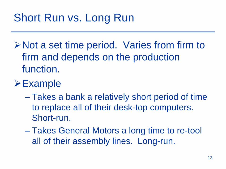
Short Run vs. Long Run
Not a set time period. Varies from firm to firm and depends on the production function.Example
– Takes a bank a relatively short period of time to replace all of their desk-top computers. Short-run.
– Takes General Motors a long time to re-tool all of their assembly lines. Long-run.
13
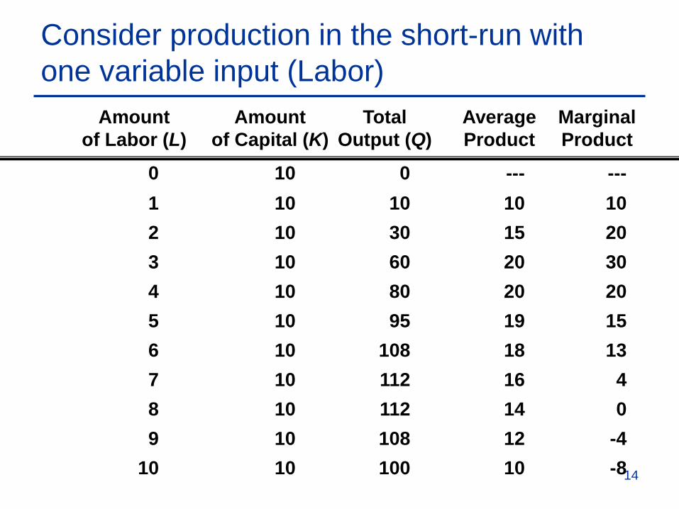
Consider production in the short-run with one variable input (Labor)
Amount Amount Total Average Marginalof Labor (L) of Capital (K) Output (Q) Product Product
0 10 0 --- ---1 10 10 10 102 10 30 15 203 10 60 20 304 10 80 20 205 10 95 19 156 10 108 18 137 10 112 16 48 10 112 14 09 10 108 12 -4
10 10 100 10 -814

Production with one variable input (Labor)
With additional workers output (Q) initially increases, reaches a maximum, and then decreases.The average product of labor (AP), or
output per worker, increases and then decreases.
LQ
Input LaborOutput AP ==
15
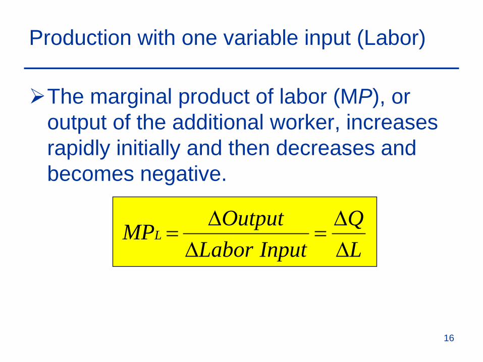
Production with one variable input (Labor)
The marginal product of labor (MP), or output of the additional worker, increases rapidly initially and then decreases and becomes negative.
LQ
Input LaborOutput MPL
∆∆
=∆∆
=
16
Production with one variable input (Labor)
Total Product
A: slope of tangent = MP (20)B: slope of 0B = AP (20)C: slope of 0C= MP & AP
Labor per Month
Outputper
Month
60
112
0 2 3 4 5 6 7 8 9 101
A
B
C
D
17
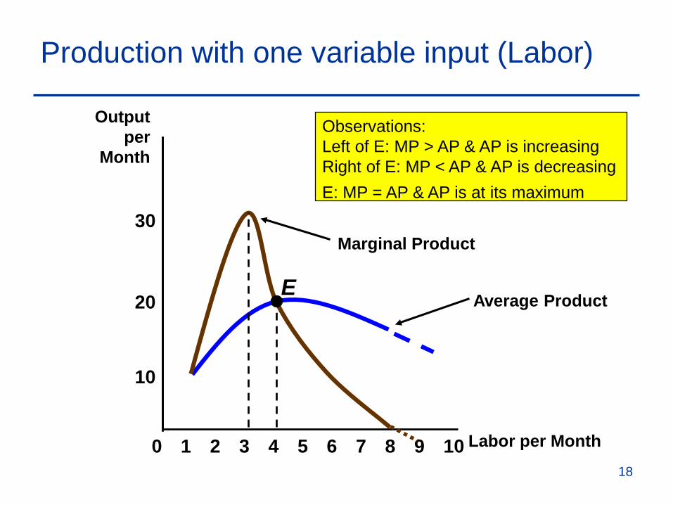
Production with one variable input (Labor)
Average Product
8
10
20
Outputper
Month
0 2 3 4 5 6 7 9 101 Labor per Month
30
E
Marginal Product
Observations:Left of E: MP > AP & AP is increasingRight of E: MP < AP & AP is decreasingE: MP = AP & AP is at its maximum
18
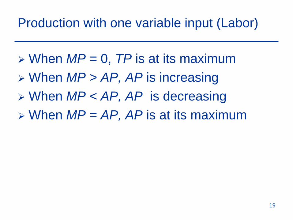
Production with one variable input (Labor)
When MP = 0, TP is at its maximum When MP > AP, AP is increasing When MP < AP, AP is decreasing When MP = AP, AP is at its maximum
19
Production with one variable input (Labor)
As the use of an input increases in equal increments, a point will be reached at which the resulting additions to output decreases (i.e. MP declines).Known as the Law of Diminishing Marginal
Returns.
20
Law of Diminishing Marginal Returns
When the labor input is small, MP increases due to specialization.
When the labor input is large, MPdecreases due to inefficiencies.
21

Production with one variable input (Labor)
Assumes the quality of the variable input is constant.
Explains a declining MP, not necessarily a negative one
Assumes a constant technology
22
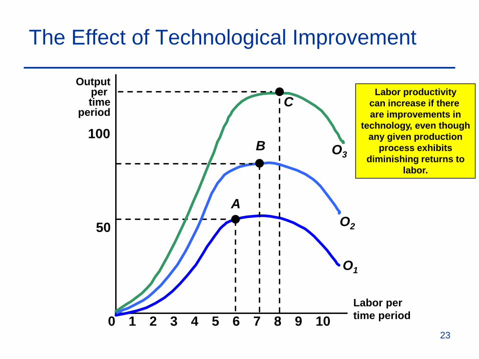
The Effect of Technological Improvement
Labor pertime period
Outputper time
period
50
100
0 2 3 4 5 6 7 8 9 101
A
O1
C
O3
O2
B
Labor productivitycan increase if there are improvements in
technology, even thoughany given production
process exhibitsdiminishing returns to
labor.
23
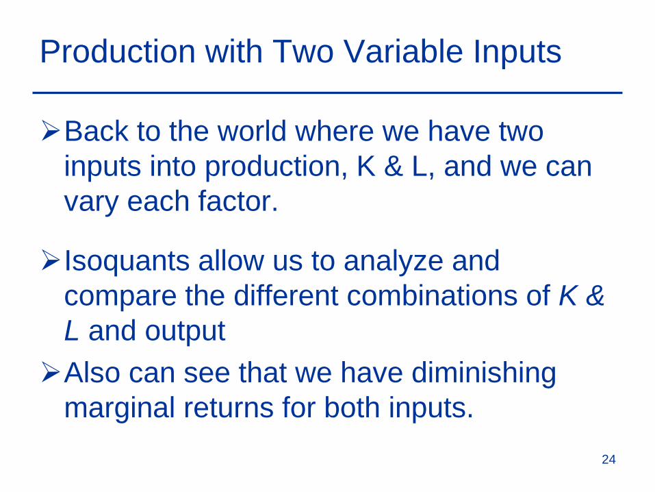
Production with Two Variable Inputs
Back to the world where we have two inputs into production, K & L, and we can vary each factor.
Isoquants allow us to analyze and compare the different combinations of K & L and outputAlso can see that we have diminishing
marginal returns for both inputs.24
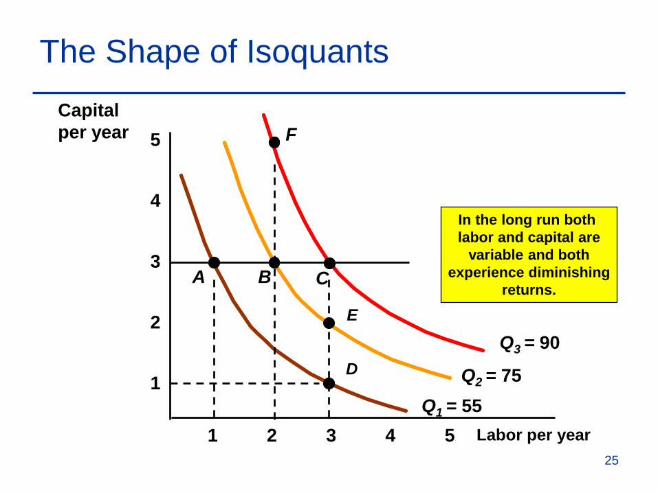
The Shape of Isoquants
Labor per year
1
2
3
4
1 2 3 4 5
5
In the long run both labor and capital are
variable and bothexperience diminishing
returns.
Q1 = 55Q2 = 75
Q3 = 90
Capitalper year
A
D
B C
F
E
25
Production with Two Variable Inputs
Assume capital is 3 and labor increases from 0 to 1 to 2 to 3 (A→B→C). – Notice output increases at a decreasing rate
(55, 20, 15) illustrating diminishing returns from labor in the short-run and long-run.
Assume labor is 3 and capital increases from 0 to 1 to 2 to 3 (D→E→C).– Output also increases at a decreasing rate
(55, 20, 15) due to diminishing returns from capital.
26
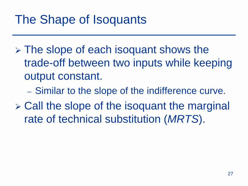
The Shape of Isoquants
The slope of each isoquant shows the trade-off between two inputs while keeping output constant.– Similar to the slope of the indifference curve.
Call the slope of the isoquant the marginal rate of technical substitution (MRTS).
27
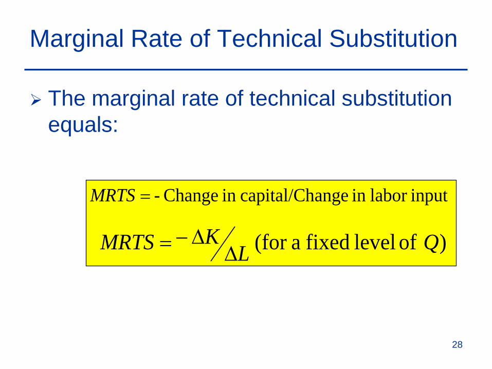
Marginal Rate of Technical Substitution
The marginal rate of technical substitution equals:
inputlabor in angecapital/Chin Change - MRTS =
) of level fixed a(for QLK MRTS ∆
∆−=
28
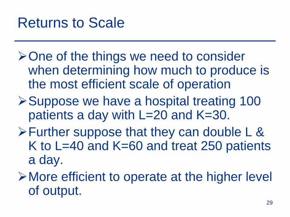
Returns to Scale
One of the things we need to consider when determining how much to produce is the most efficient scale of operationSuppose we have a hospital treating 100
patients a day with L=20 and K=30.Further suppose that they can double L &
K to L=40 and K=60 and treat 250 patients a day.More efficient to operate at the higher level
of output.29
Returns to scale
Returns to Scale measures the relationship between the scale or size of a firm and output.
3 possibilities.
30
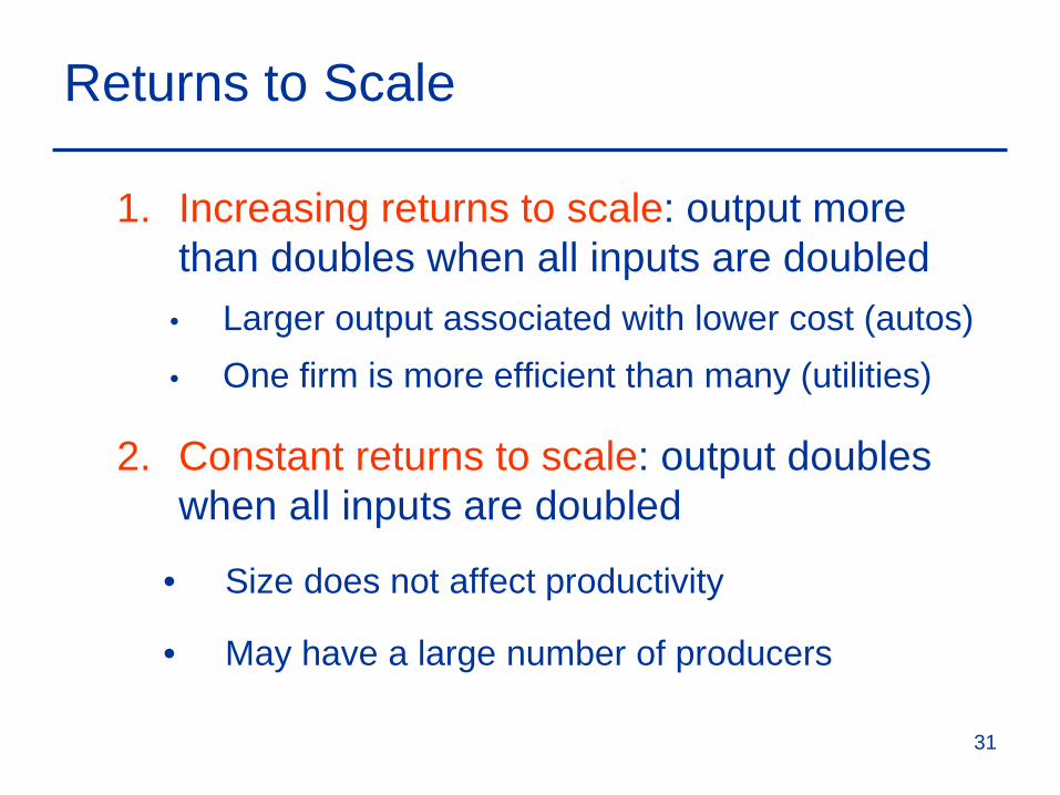
Returns to Scale
1. Increasing returns to scale: output more than doubles when all inputs are doubled
• Larger output associated with lower cost (autos)• One firm is more efficient than many (utilities)
2. Constant returns to scale: output doubles when all inputs are doubled
• Size does not affect productivity
• May have a large number of producers
31
Returns to Scale
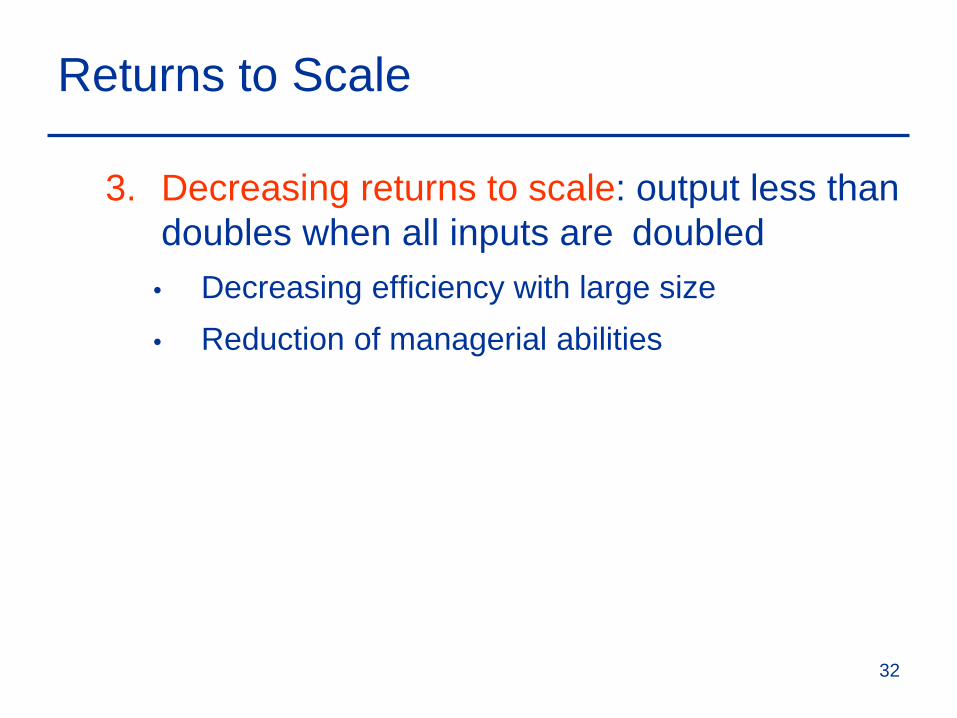
3. Decreasing returns to scale: output less than doubles when all inputs are doubled
• Decreasing efficiency with large size• Reduction of managerial abilities
32
Returns to Scale
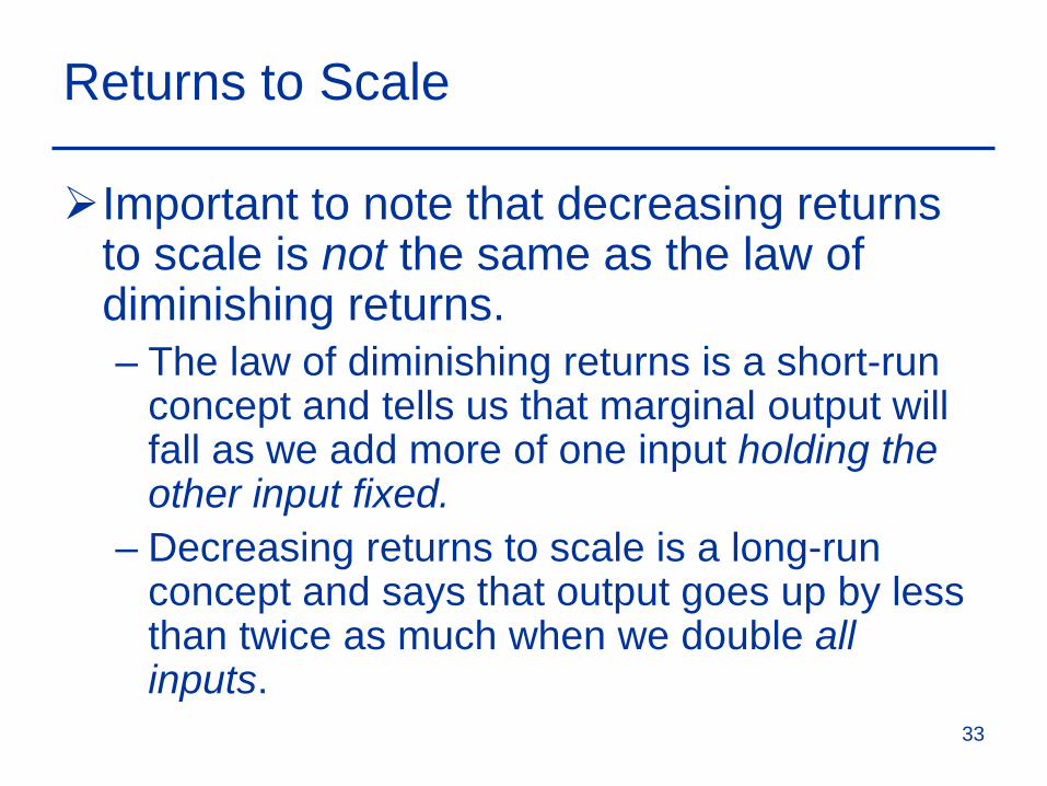
Important to note that decreasing returns to scale is not the same as the law of diminishing returns. – The law of diminishing returns is a short-run
concept and tells us that marginal output will fall as we add more of one input holding the other input fixed.
– Decreasing returns to scale is a long-run concept and says that output goes up by less than twice as much when we double all inputs.
33
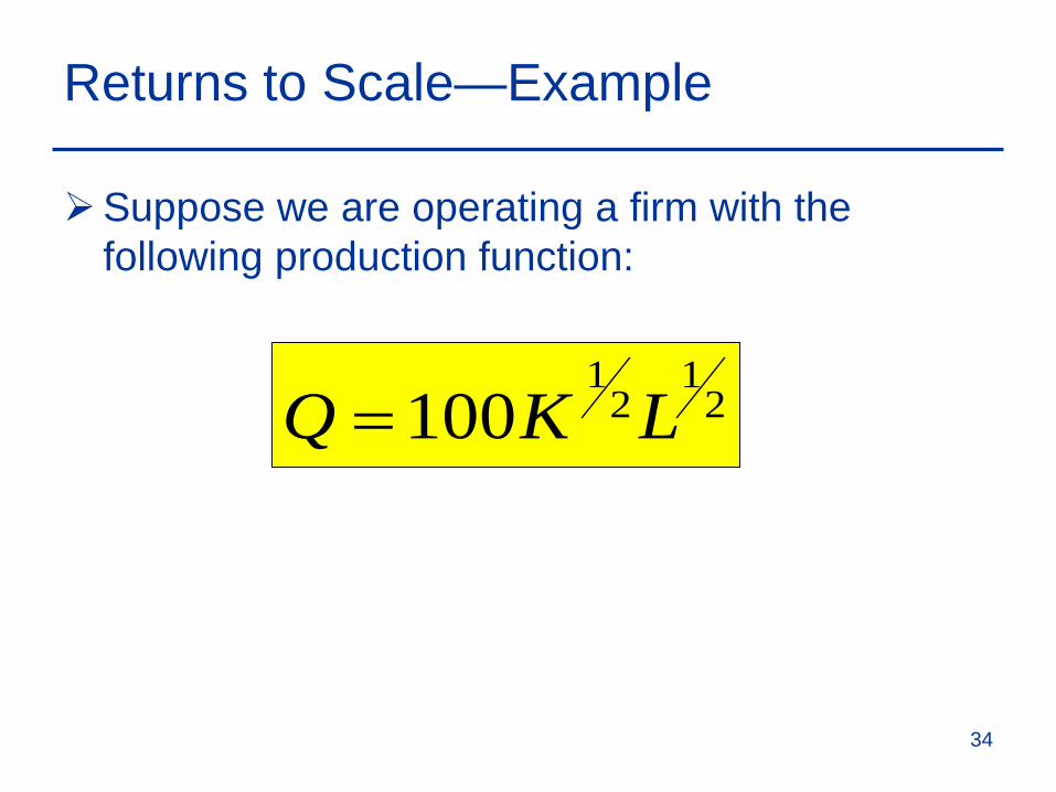
Returns to Scale—Example
Suppose we are operating a firm with the following production function:
21
21
100 LKQ =
34
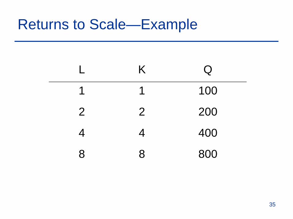
Returns to Scale—Example
L K Q
1 1 100
2 2 200
4 4 400
8 8 800
35

Returns to Scale—Example
Now consider the following production function:
LKQ 21
100=
36
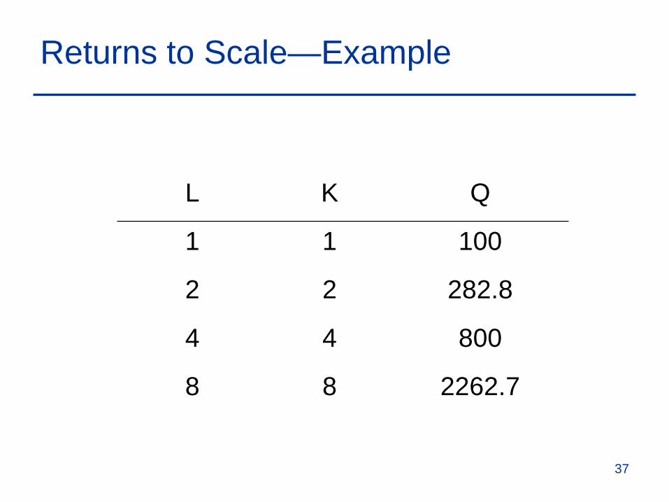
L K Q
1 1 100
2 2 282.8
4 4 800
8 8 2262.7
Returns to Scale—Example
37
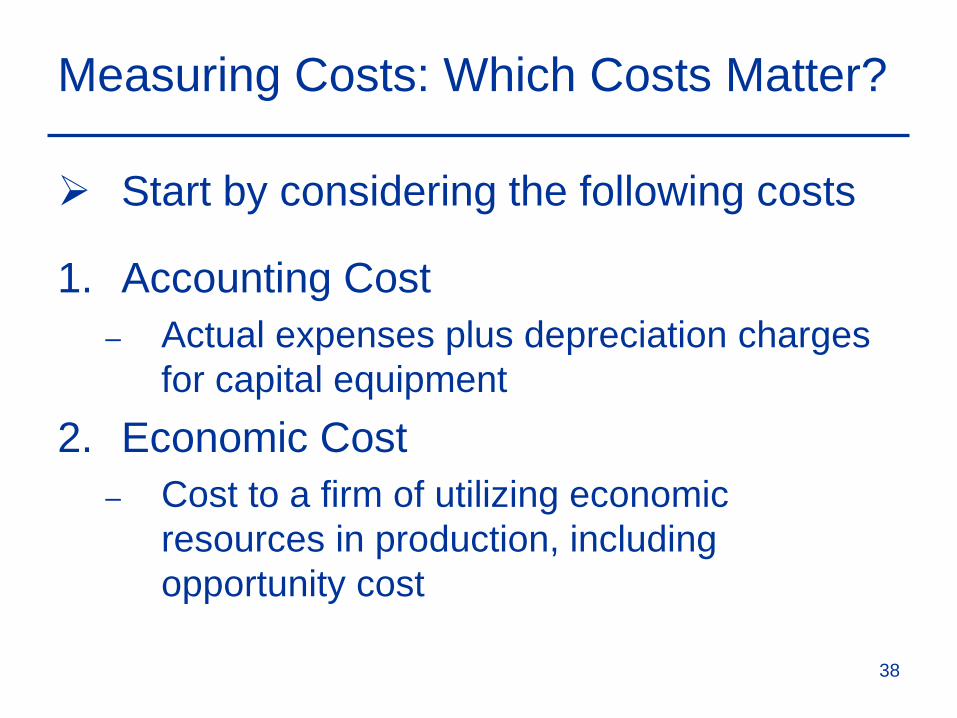
Measuring Costs: Which Costs Matter?
Start by considering the following costs
1. Accounting Cost– Actual expenses plus depreciation charges
for capital equipment2. Economic Cost
– Cost to a firm of utilizing economic resources in production, including opportunity cost
38
Opportunity Cost
Opportunity Cost is the value of a resource when the resource is employed in it’s best alternative use.
39
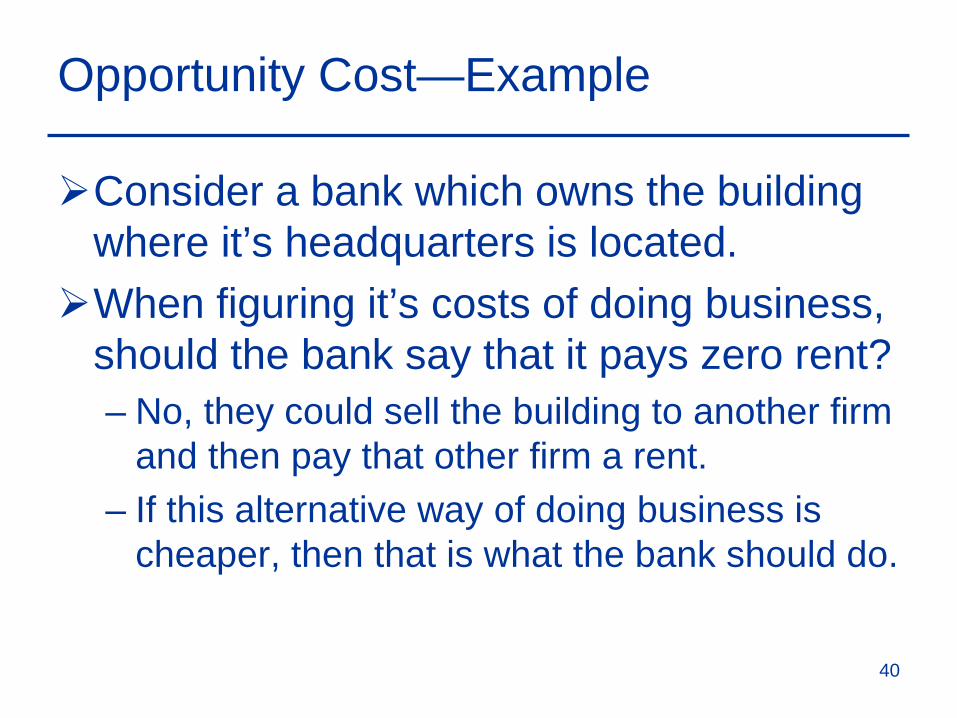
Opportunity Cost—Example
Consider a bank which owns the building where it’s headquarters is located.When figuring it’s costs of doing business,
should the bank say that it pays zero rent?– No, they could sell the building to another firm
and then pay that other firm a rent.– If this alternative way of doing business is
cheaper, then that is what the bank should do.
40
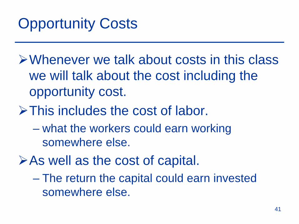
Opportunity Costs
Whenever we talk about costs in this class we will talk about the cost including the opportunity cost. This includes the cost of labor.
– what the workers could earn working somewhere else.
As well as the cost of capital.– The return the capital could earn invested
somewhere else.41
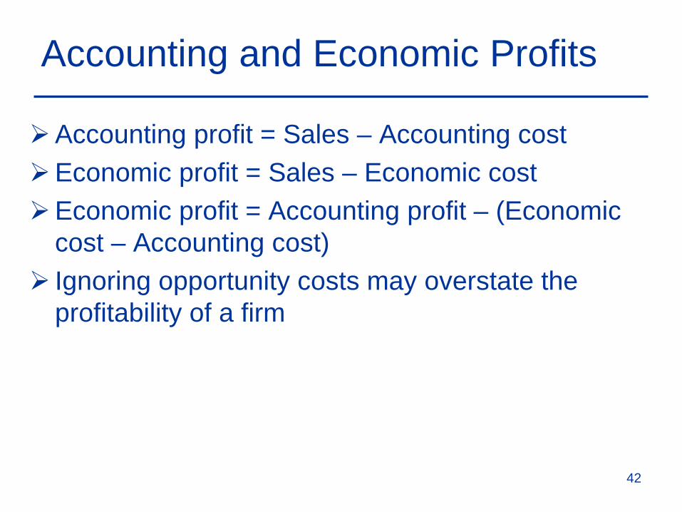
Accounting and Economic Profits
Accounting profit = Sales – Accounting costEconomic profit = Sales – Economic costEconomic profit = Accounting profit – (Economic
cost – Accounting cost) Ignoring opportunity costs may overstate the
profitability of a firm
42
Sunk Cost
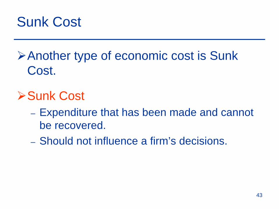
Another type of economic cost is Sunk Cost.
Sunk Cost– Expenditure that has been made and cannot
be recovered. – Should not influence a firm’s decisions.
43
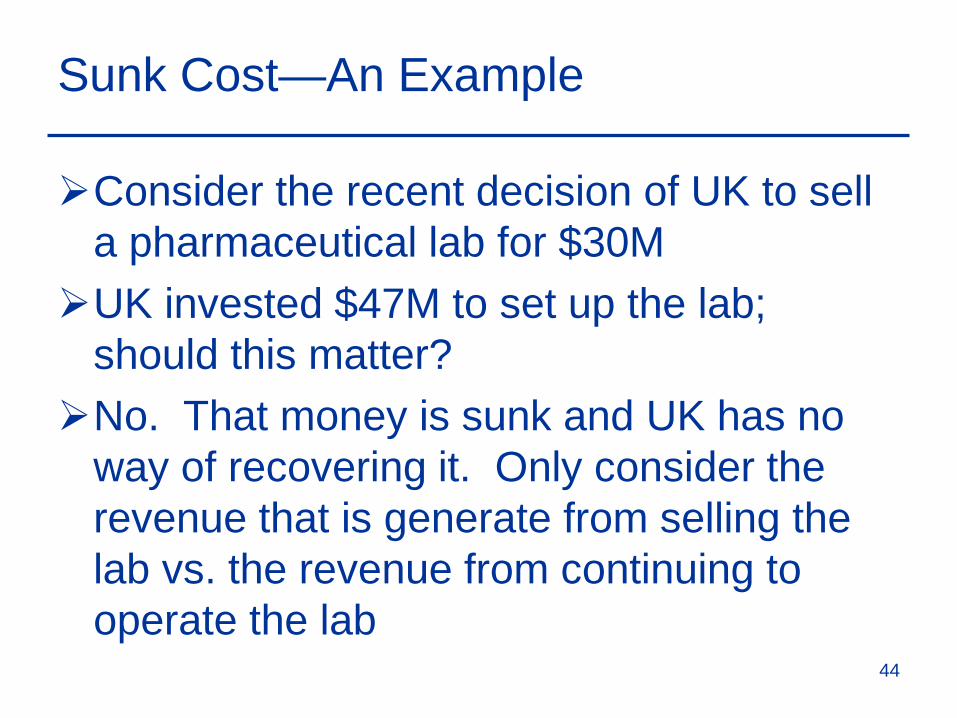
Sunk Cost—An Example
Consider the recent decision of UK to sell a pharmaceutical lab for $30MUK invested $47M to set up the lab;
should this matter?No. That money is sunk and UK has no
way of recovering it. Only consider the revenue that is generate from selling the lab vs. the revenue from continuing to operate the lab
44
Sunk Cost—An Example
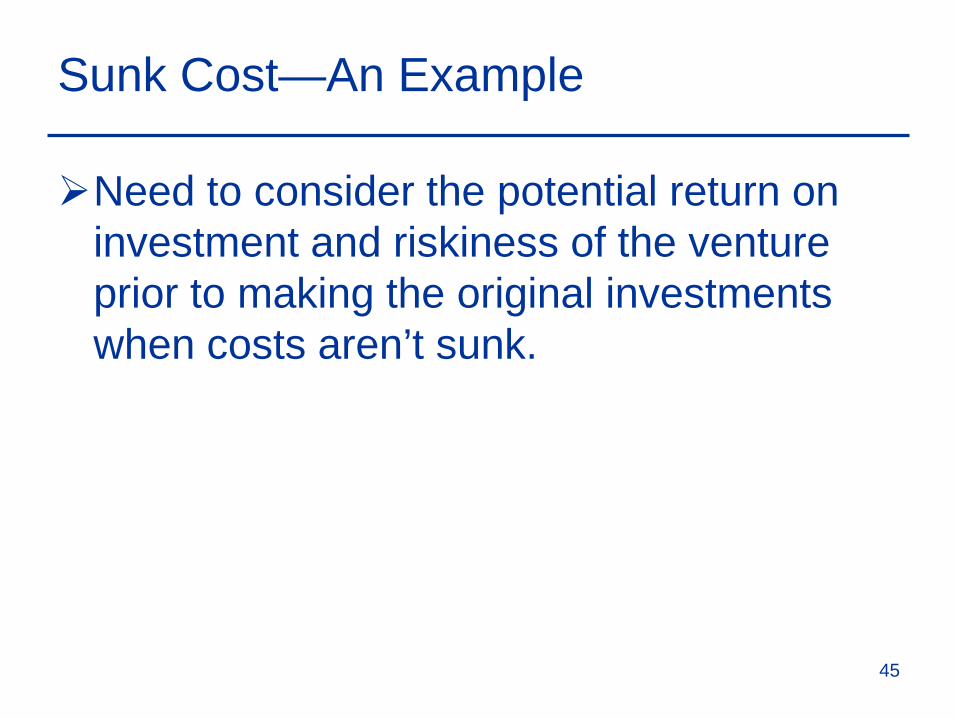
Need to consider the potential return on investment and riskiness of the venture prior to making the original investments when costs aren’t sunk.
45
Measuring Costs: Which Costs Matter?
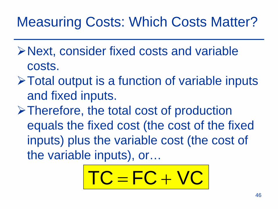
Next, consider fixed costs and variable costs.Total output is a function of variable inputs
and fixed inputs. Therefore, the total cost of production
equals the fixed cost (the cost of the fixed inputs) plus the variable cost (the cost of the variable inputs), or…
VC FC TC +=46

Measuring Costs: Which Costs Matter?
Fixed Cost (FC)
– Does not vary with the level of output
Variable Cost (VC)
– Cost that varies as output varies
47
Measuring Costs: Which Costs Matter?
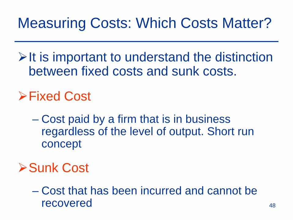
It is important to understand the distinction between fixed costs and sunk costs.
Fixed Cost
– Cost paid by a firm that is in business regardless of the level of output. Short run concept
Sunk Cost
– Cost that has been incurred and cannot be recovered 48
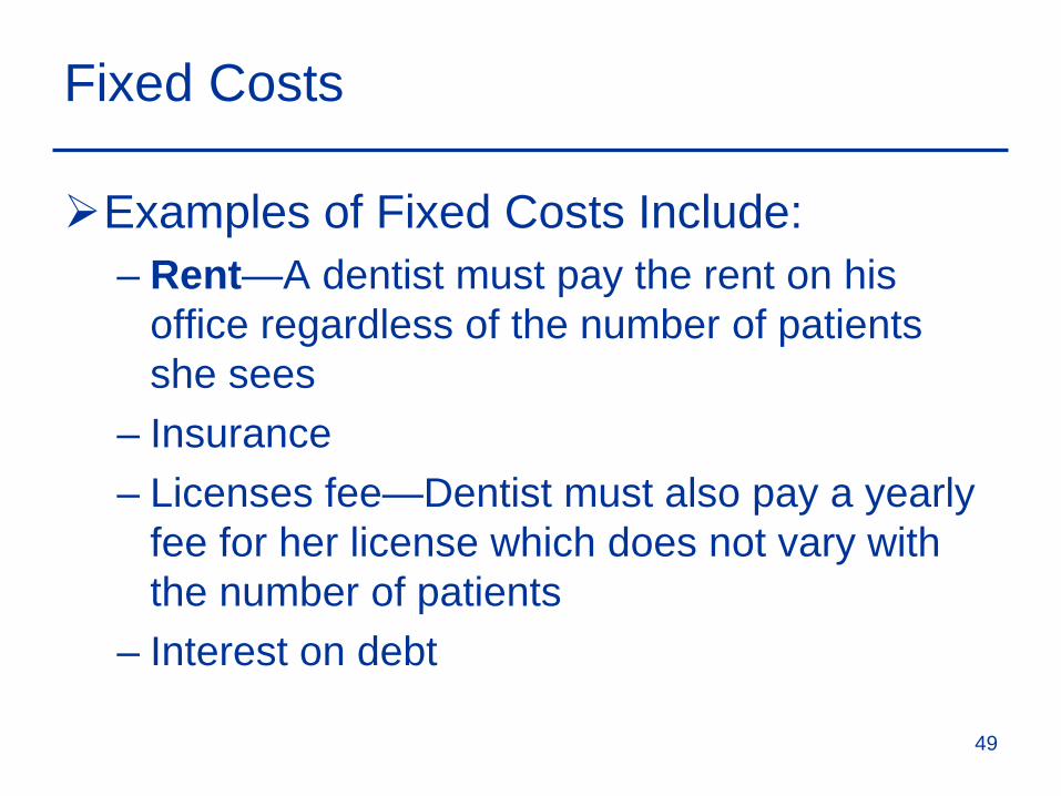
Fixed Costs
Examples of Fixed Costs Include:– Rent—A dentist must pay the rent on his
office regardless of the number of patients she sees
– Insurance– Licenses fee—Dentist must also pay a yearly
fee for her license which does not vary with the number of patients
– Interest on debt
49
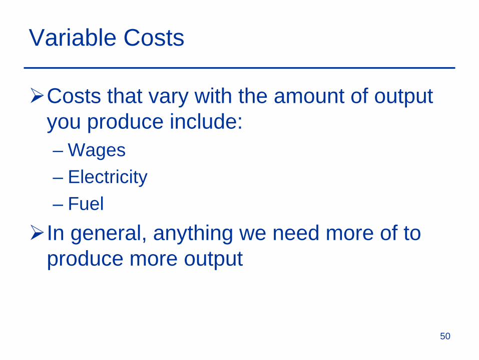
Variable Costs
Costs that vary with the amount of output you produce include:– Wages– Electricity– Fuel
In general, anything we need more of to produce more output
50
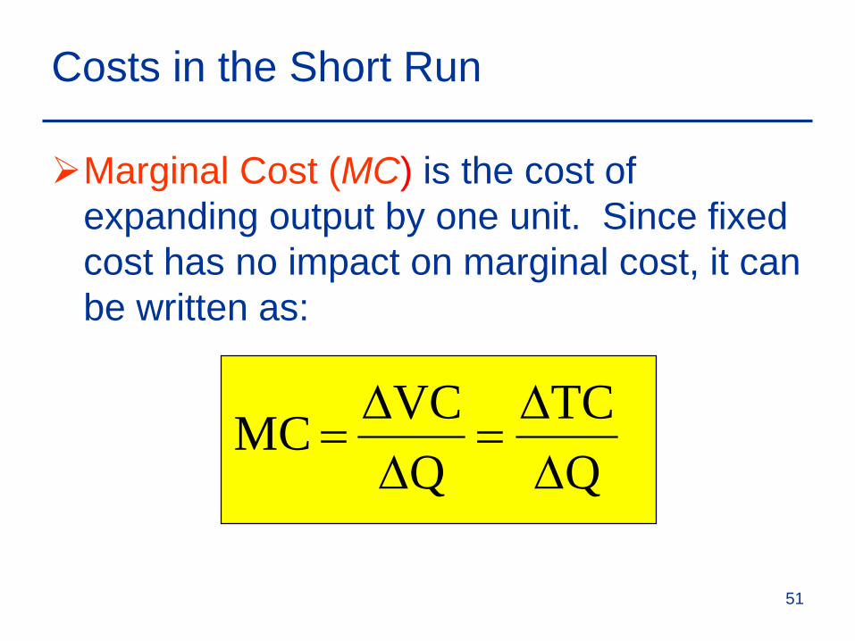
Costs in the Short Run
Marginal Cost (MC) is the cost of expanding output by one unit. Since fixed cost has no impact on marginal cost, it can be written as:
QTC
QVC MC
∆∆
=∆∆
=
51
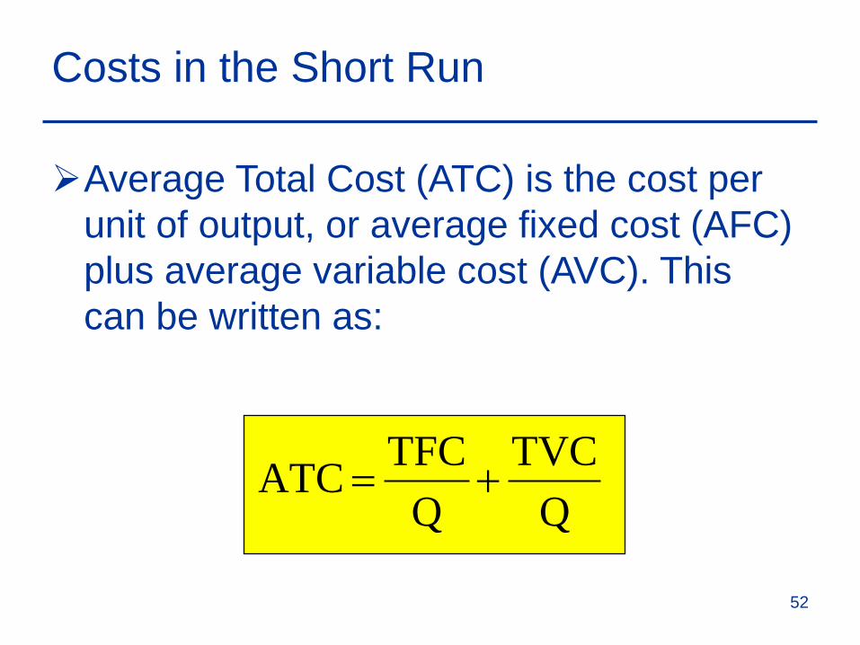
Costs in the Short Run
Average Total Cost (ATC) is the cost per unit of output, or average fixed cost (AFC) plus average variable cost (AVC). This can be written as:
QTVC
QTFC ATC +=
52
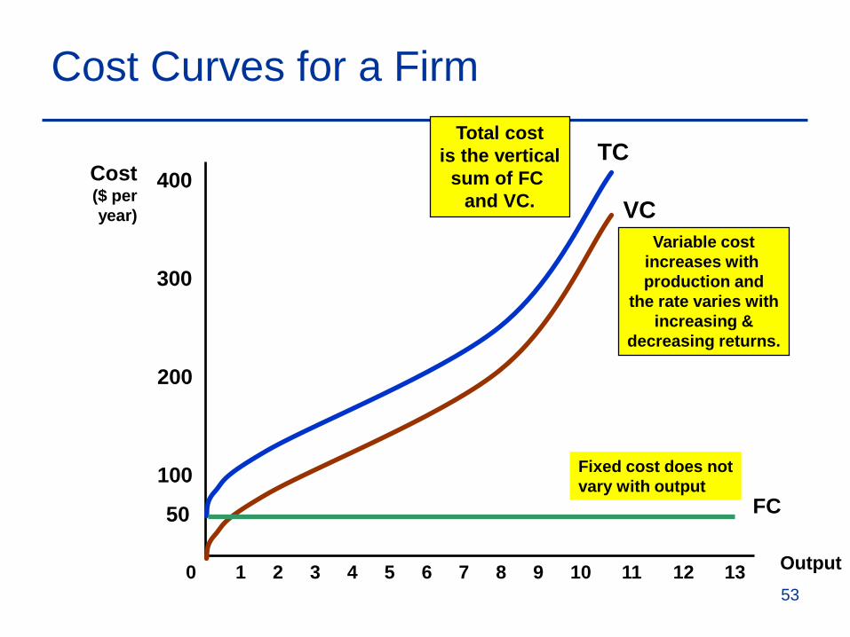
Cost Curves for a Firm
Output
Cost($ peryear)
100
200
300
400
0 1 2 3 4 5 6 7 8 9 10 11 12 13
VCVariable cost
increases with production and
the rate varies withincreasing &
decreasing returns.
TCTotal cost
is the verticalsum of FC
and VC.
FC50
Fixed cost does notvary with output
53
Cost Curves for a Firm
Output (units/yr.)
Cost($ perunit)
25
50
75
100
0 1 2 3 4 5 6 7 8 9 10 11
MC
ATCAVC
AFC
54
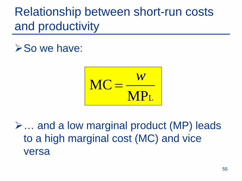
Relationship between short-run costs and productivity
So we have:
… and a low marginal product (MP) leads to a high marginal cost (MC) and vice versa
LMP MC w=
55
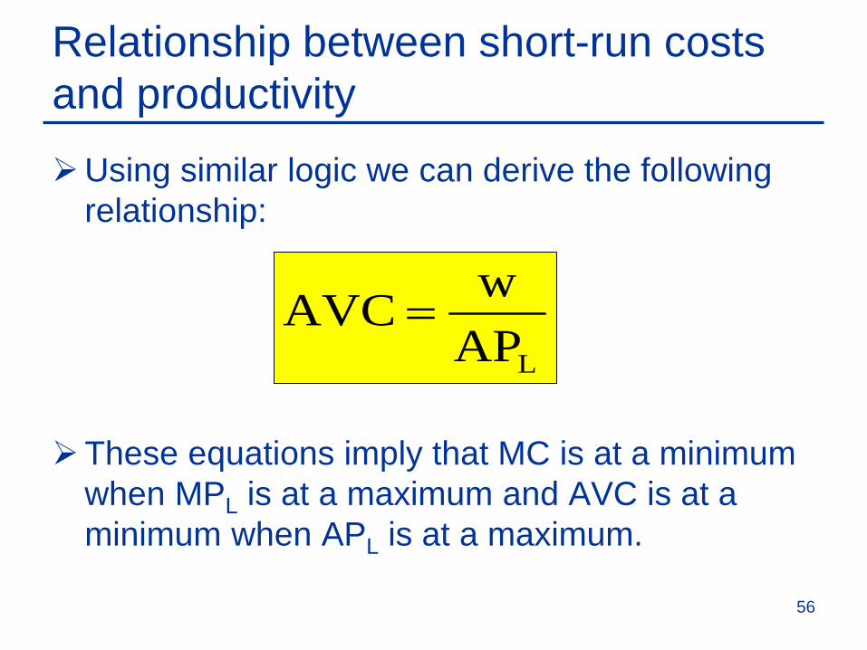
Relationship between short-run costs and productivity
Using similar logic we can derive the following relationship:
These equations imply that MC is at a minimum when MPL is at a maximum and AVC is at a minimum when APL is at a maximum.
LAPwAVC =
56
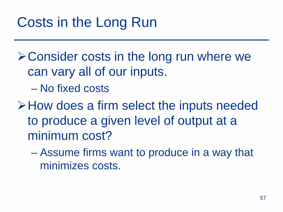
Costs in the Long Run
Consider costs in the long run where we can vary all of our inputs.– No fixed costs
How does a firm select the inputs needed to produce a given level of output at a minimum cost?– Assume firms want to produce in a way that
minimizes costs.
57
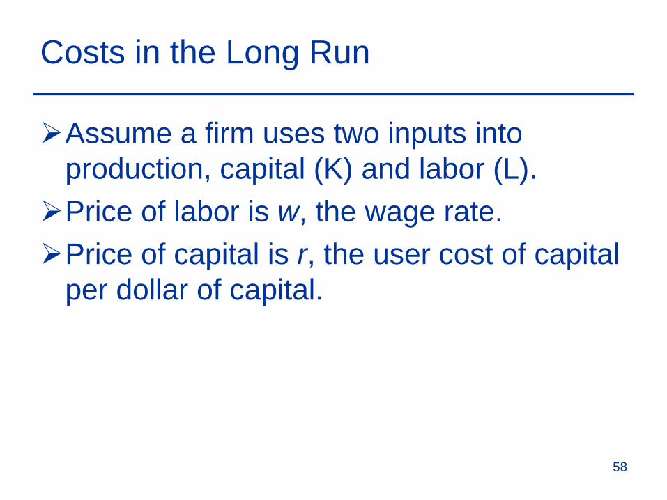
Costs in the Long Run
Assume a firm uses two inputs into production, capital (K) and labor (L).Price of labor is w, the wage rate.Price of capital is r, the user cost of capital
per dollar of capital.
58
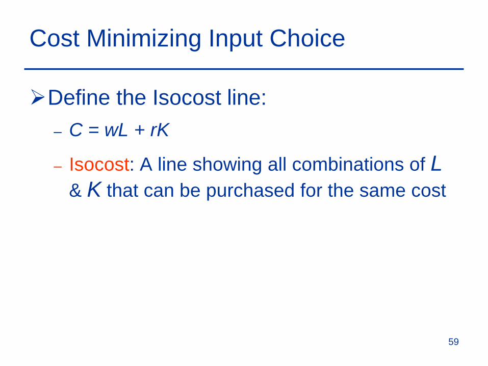
Cost Minimizing Input Choice
Define the Isocost line:– C = wL + rK
– Isocost: A line showing all combinations of L& K that can be purchased for the same cost
59
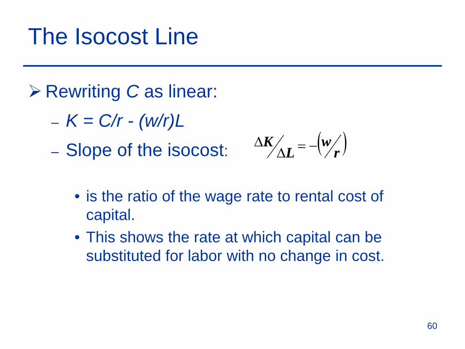
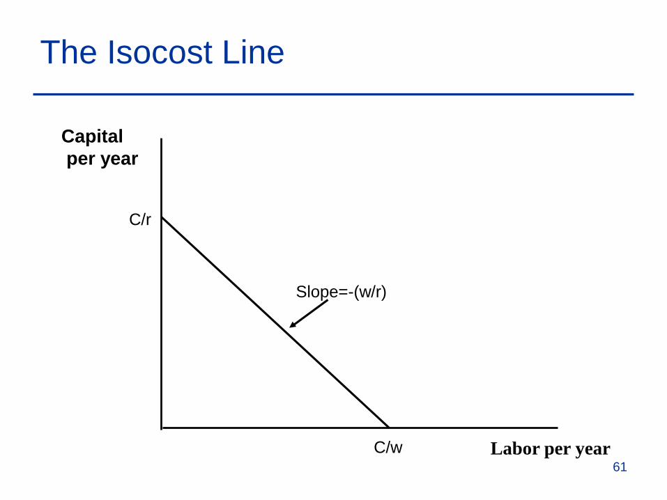
The Isocost Line
Rewriting C as linear:– K = C/r - (w/r)L– Slope of the isocost:
• is the ratio of the wage rate to rental cost of capital.
• This shows the rate at which capital can be substituted for labor with no change in cost.
( )rw
LK −=∆
∆
60
The Isocost Line
Labor per year
Capitalper year
C/r
C/w
Slope=-(w/r)
61

The Isocost Line
Suppose, w=$36,000/year and r=$18,000/year. What does the budget line look like when
C=$180,000/year?
62
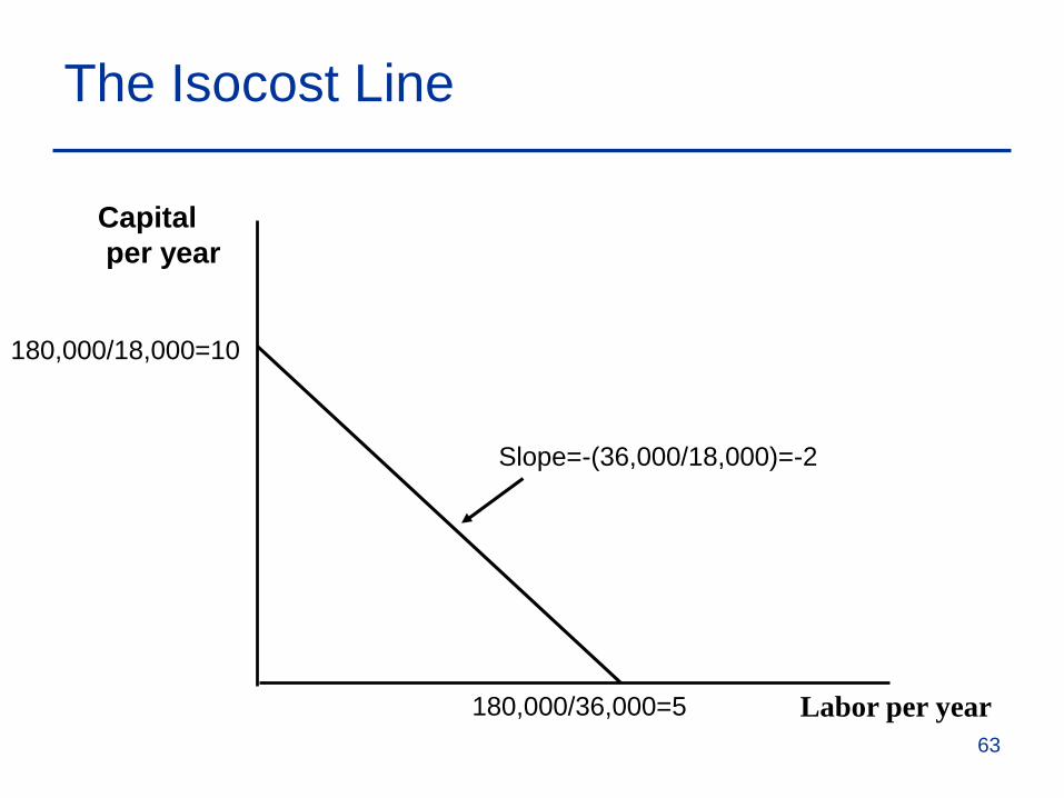
The Isocost Line
Labor per year
Capitalper year
180,000/18,000=10
180,000/36,000=5
Slope=-(36,000/18,000)=-2
63
Cost Minimizing Input Choice
In order to choose the cost minimizing input choice we combined the isocost line with the isoquant.
64
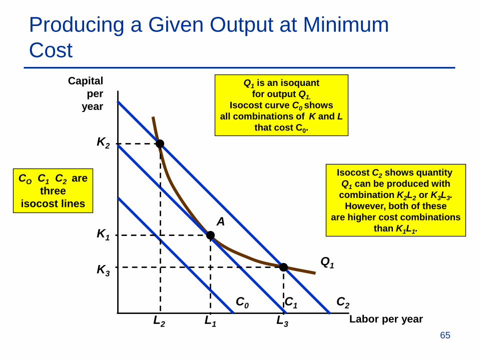
Producing a Given Output at Minimum Cost
Labor per year
Capital per
year
Isocost C2 shows quantity Q1 can be produced withcombination K2L2 or K3L3.
However, both of theseare higher cost combinations
than K1L1.
Q1
Q1 is an isoquantfor output Q1.
Isocost curve C0 showsall combinations of K and L
that cost C0.
C0 C1 C2
CO C1 C2 arethree
isocost linesA
K1
L1
K3
L3
K2
L265

Costs in the Long Run
Relationship between Isoquants and Isocosts and the Production Function
rw
MPMP
K
L =
L
K
MPKMRTS L MP∆= − = −∆
Slope of isocost line wKL r
∆= − = −∆
66
Costs in the Long Run
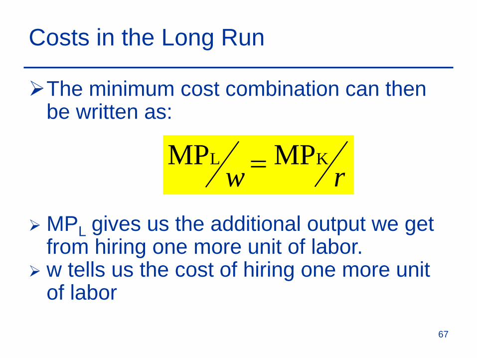
The minimum cost combination can then be written as:
MPL gives us the additional output we get from hiring one more unit of labor.
w tells us the cost of hiring one more unit of labor
rwKL MPMP =
67
Costs in the Long Run
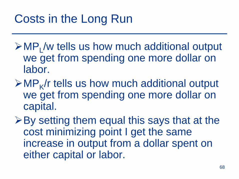
MPL/w tells us how much additional output we get from spending one more dollar on labor.MPK/r tells us how much additional output
we get from spending one more dollar on capital.By setting them equal this says that at the
cost minimizing point I get the same increase in output from a dollar spent on either capital or labor.
68
Input Substitution When an InputPrice Changes
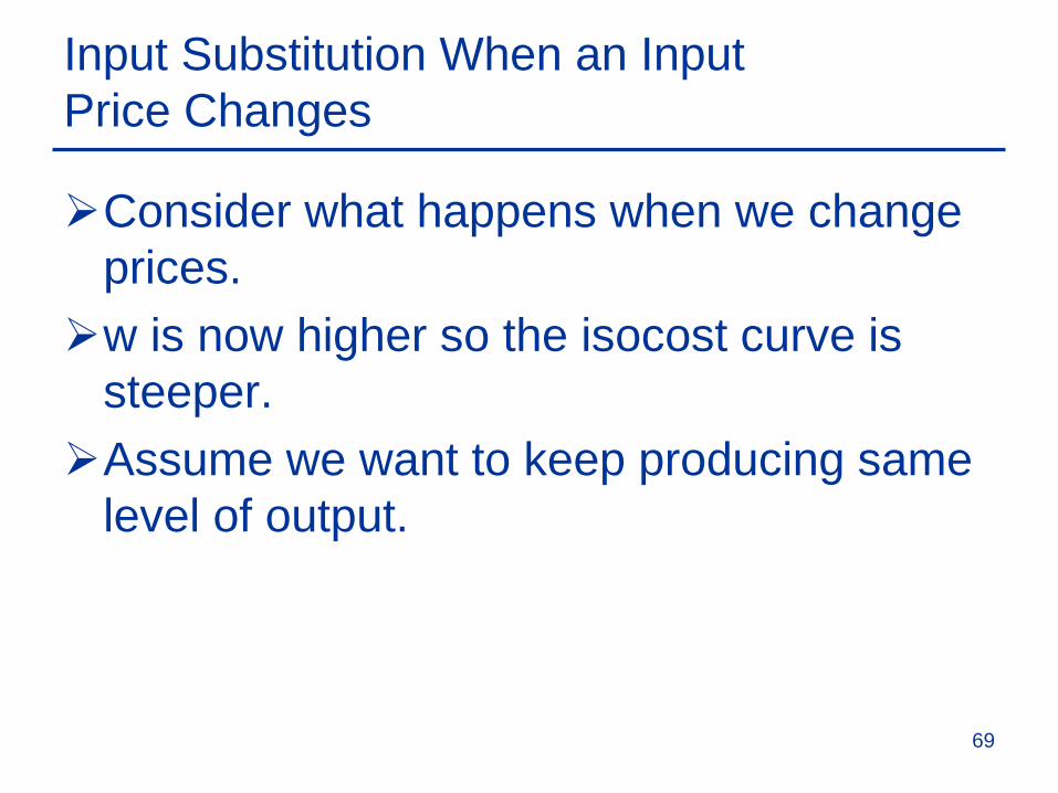
Consider what happens when we change prices.w is now higher so the isocost curve is
steeper.Assume we want to keep producing same
level of output.
69
Input Substitution When an InputPrice Changes
C2
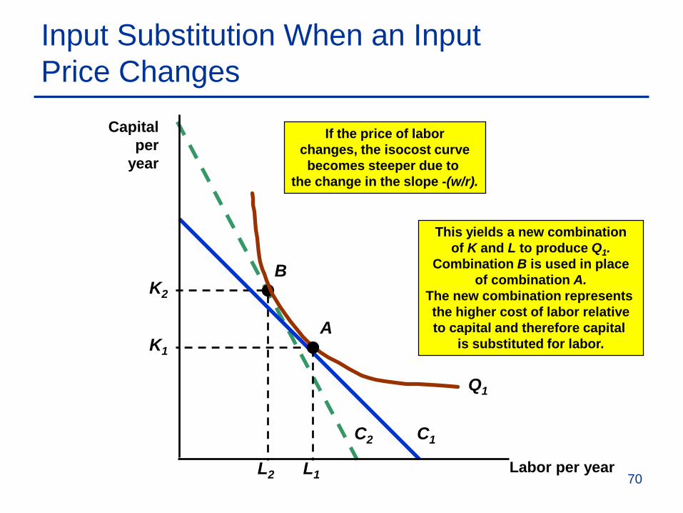
This yields a new combinationof K and L to produce Q1.
Combination B is used in placeof combination A.
The new combination represents the higher cost of labor relativeto capital and therefore capital
is substituted for labor.
K2
L2
B
C1
K1
L1
A
Q1
If the price of laborchanges, the isocost curvebecomes steeper due to
the change in the slope -(w/r).
Labor per year
Capitalper
year
70
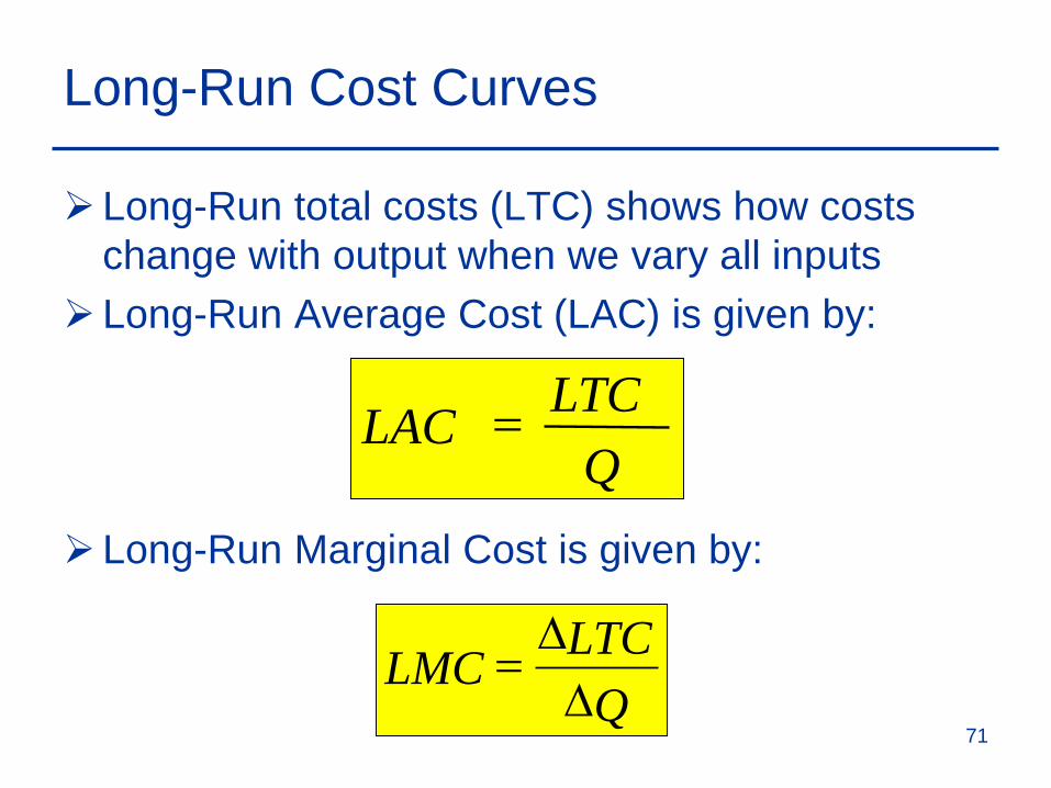
Long-Run Cost Curves
Long-Run total costs (LTC) shows how costs change with output when we vary all inputs
Long-Run Average Cost (LAC) is given by:
Long-Run Marginal Cost is given by:
QLTCLAC =
QLTCLMC∆
∆=
71
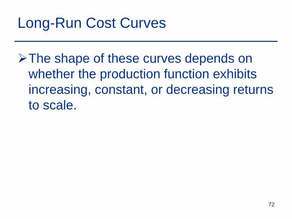
Long-Run Cost Curves
The shape of these curves depends on whether the production function exhibits increasing, constant, or decreasing returns to scale.
72

Long-Run Average Cost (LAC)
Constant Returns to Scale– If input is doubled, output will double and
average cost is constant at all levels of output.– LAC curve will be a flat line.
Increasing Returns to Scale– If input is doubled, output will more than
double and average cost decreases at all levels of output.
– LAC curve is downward sloping.
73

Long-Run Average Cost (LAC)
Decreasing Returns to Scale– If input is doubled, the increase in output is
less than twice as large and average cost increases with output.
– LAC curve is upward sloping.
74
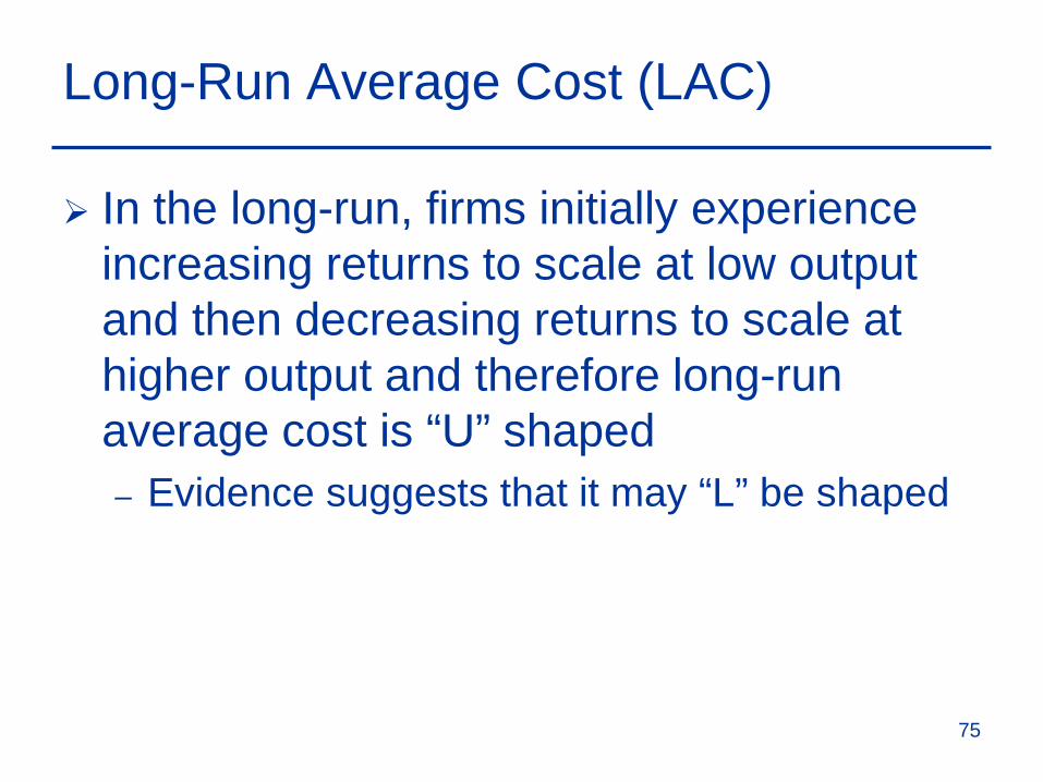
Long-Run Average Cost (LAC)
In the long-run, firms initially experience increasing returns to scale at low output and then decreasing returns to scale at higher output and therefore long-run average cost is “U” shaped– Evidence suggests that it may “L” be shaped
75
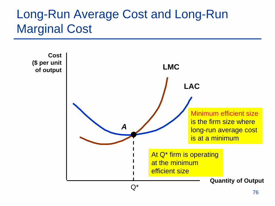
Long-Run Average Cost and Long-RunMarginal Cost
Quantity of Output
Cost($ per unitof output
LAC
LMC
A
Q*
At Q* firm is operating at the minimum efficient size
Minimum efficient size is the firm size where long-run average cost is at a minimum
76
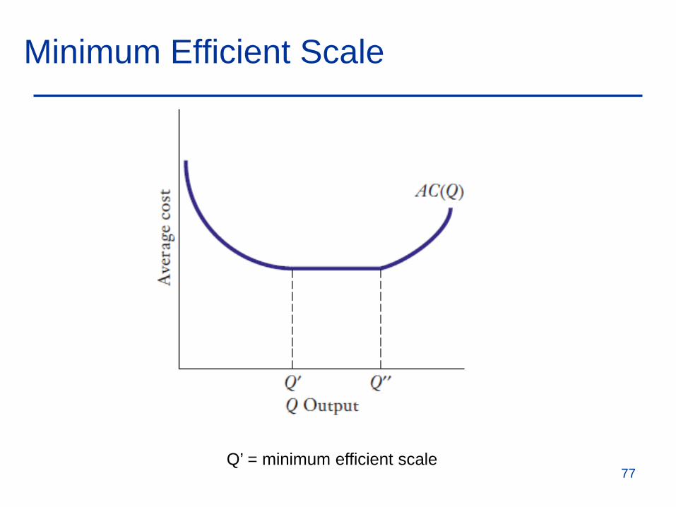
Minimum Efficient Scale
Q’ = minimum efficient scale77
Minimum Efficient Scale
Number of firms in an industry is determined by the minimum efficient scale of production and the market demand for the product.
78

Summary
A production function describes the maximum output a firm can produce for each specified combination of inputs.
An isoquant is a curve that shows all combinations of inputs that yield a given level of output.
79
Summary
Average product of labor measures the productivity of the average worker, whereas marginal product of labormeasures the productivity of the last worker added.
The law of diminishing returns explains that the marginal product of an input eventually diminishes as its quantity is increased.
80
Summary
Managers must take into account the opportunity cost associated with the use of the firm’s resources.
Firms are faced with both fixed and variable costs in the short-run.
81
Summary
When there is a single variable input, as in the short run, the presence of diminishing returns determines the shape of the cost curves.In the long run, all inputs to the production
process are variable.A firm enjoys economies of scale when it
can double its output at less than twice the cost.
82
Summary
In long-run analysis, we focus on the firm’s choice of its scale or size of operation.
83