Lecture 2: The SVM classifierC19 Machine Learning Hilary 2015 A. Zisserman

• Review of linear classifiers • Linear separability• Perceptron

• Support Vector Machine (SVM) classifier • Wide margin • Cost function• Slack variables• Loss functions revisited• Optimization

Binary Classification

Given training data (xi, yi) for i = 1 . . . N , with

xi ∈ Rd and yi ∈ {−1,1}, learn a classifier f(x)such that

f(xi)

(≥ 0 yi = +1< 0 yi = −1

i.e. yif(xi) > 0 for a correct classification.

Linear separability

linearly separable

not linearly

separable

Linear classifiers

X2

X1

A linear classifier has the form

• in 2D the discriminant is a line

• is the normal to the line, and b the bias

• is known as the weight vector

f(x) = 0

f(x) = w>x+ b

f(x) > 0f(x) < 0

Linear classifiers

A linear classifier has the form

• in 3D the discriminant is a plane, and in nD it is a hyperplane

For a K-NN classifier it was necessary to `carry’ the training data

For a linear classifier, the training data is used to learn w and then discarded

Only w is needed for classifying new data

f(x) = 0

f(x) = w>x+ b

Given linearly separable data xi labelled into two categories yi = {-1,1} , find a weight vector w such that the discriminant function

separates the categories for i = 1, .., N• how can we find this separating hyperplane ?

The Perceptron Classifier

f(xi) = w>xi+ b

The Perceptron Algorithm

Write classifier as

• Initialize w = 0

• Cycle though the data points { xi, yi }

• if xi is misclassified then

• Until all the data is correctly classified

w← w+ α sign(f(xi))xi

f(xi) = w̃>x̃i+ w0 = w>xi

where w = (w̃, w0),xi = (x̃i,1)

For example in 2D

X2

X1

X2

X1

w

before update after update

w

NB after convergence w =PNi αixi

• Initialize w = 0

• Cycle though the data points { xi, yi }

• if xi is misclassified then

• Until all the data is correctly classified

w← w+ α sign(f(xi))xi

xi

• if the data is linearly separable, then the algorithm will converge

• convergence can be slow …

• separating line close to training data

• we would prefer a larger margin for generalization

-15 -10 -5 0 5 10

-10

-8

-6

-4

-2

0

2

4

6

8

Perceptron example

What is the best w?

• maximum margin solution: most stable under perturbations of the inputs

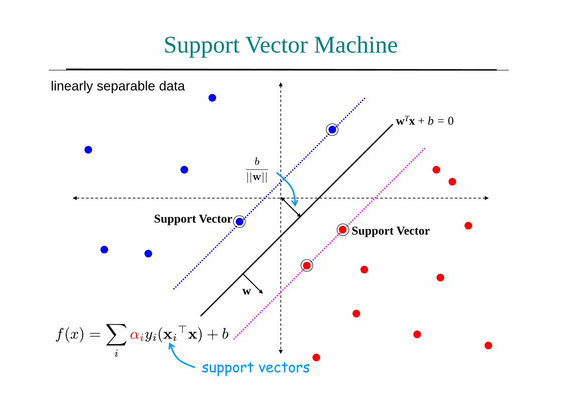
Support Vector Machine

w

Support VectorSupport Vector

b

||w||

f(x) =Xi

αiyi(xi>x) + b

support vectors

wTx + b = 0

linearly separable data

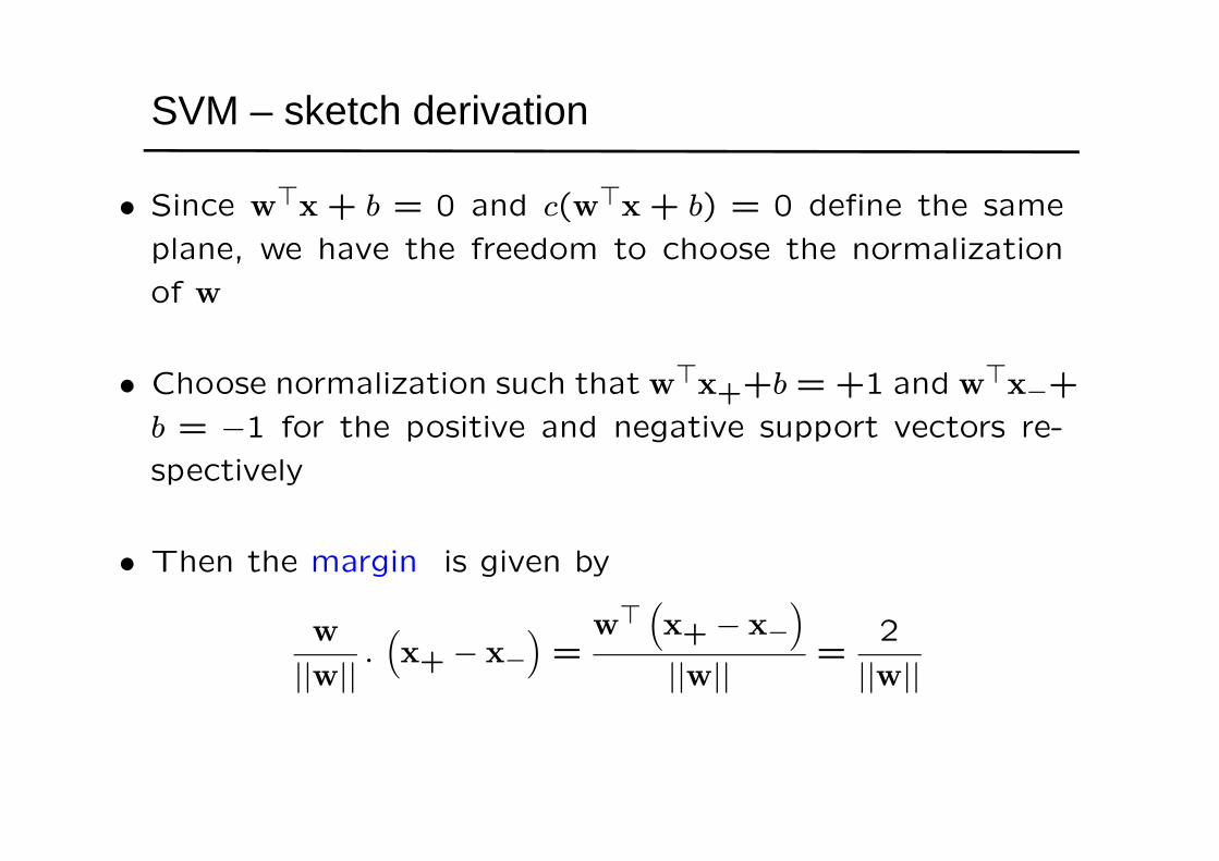
SVM – sketch derivation

• Since w>x+ b = 0 and c(w>x+ b) = 0 define the same

plane, we have the freedom to choose the normalization

of w

• Choose normalization such that w>x++b = +1 and w>x−+b = −1 for the positive and negative support vectors re-

spectively

• Then the margin is given by

w

||w|| .³x+ − x−

´=w>

³x+ − x−

´||w|| =

2

||w||

Support Vector Machine

w

Support VectorSupport Vector

wTx + b = 0

wTx + b = 1

wTx + b = -1

Margin = 2

||w||

linearly separable data

SVM – Optimization

• Learning the SVM can be formulated as an optimization:

maxw

2

||w|| subject to w>xi+b

≥ 1 if yi = +1≤ −1 if yi = −1 for i = 1 . . . N

• Or equivalently

minw||w||2 subject to yi

³w>xi+ b

´≥ 1 for i = 1 . . . N

• This is a quadratic optimization problem subject to linear

constraints and there is a unique minimum

Linear separability again: What is the best w?

• the points can be linearly separated but there is a very narrow margin

• but possibly the large margin solution is better, even though one constraint is violated

In general there is a trade off between the margin and the number of mistakes on the training data

Introduce “slack” variables

w

Support VectorSupport Vector

wTx + b = 0

wTx + b = 1

wTx + b = -1

Margin = 2

||w||Misclassified point

ξi||w|| >

2

||w||

= 0

ξi||w|| <

1

||w||

ξi ≥ 0

• for 0 < ξ ≤ 1 point is between

margin and correct side of hyper-

plane. This is amargin violation

• for ξ > 1 point is misclassified

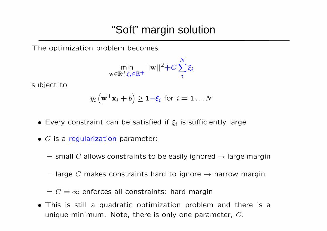
“Soft” margin solutionThe optimization problem becomes

minw∈Rd,ξi∈R+

||w||2+CNXi

ξi

subject to

yi³w>xi+ b

´≥ 1−ξi for i = 1 . . . N

• Every constraint can be satisfied if ξi is sufficiently large

• C is a regularization parameter:

— small C allows constraints to be easily ignored→ large margin

— large C makes constraints hard to ignore → narrow margin

— C =∞ enforces all constraints: hard margin

• This is still a quadratic optimization problem and there is a

unique minimum. Note, there is only one parameter, C.

-1 -0.8 -0.6 -0.4 -0.2 0 0.2 0.4 0.6 0.8-0.8

-0.6

-0.4

-0.2

0

0.2

0.4

0.6

0.8

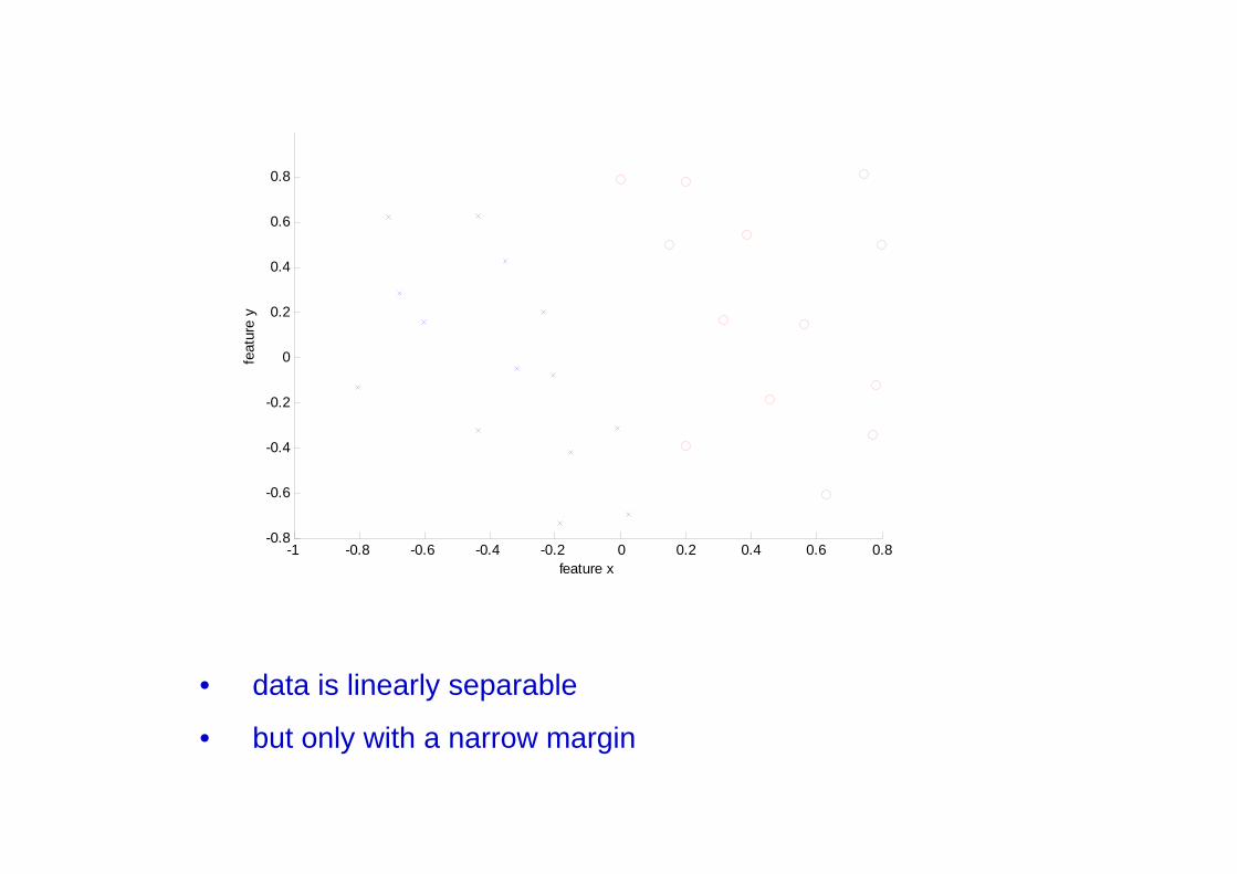
feature x

feat

ure

y

• data is linearly separable

• but only with a narrow margin

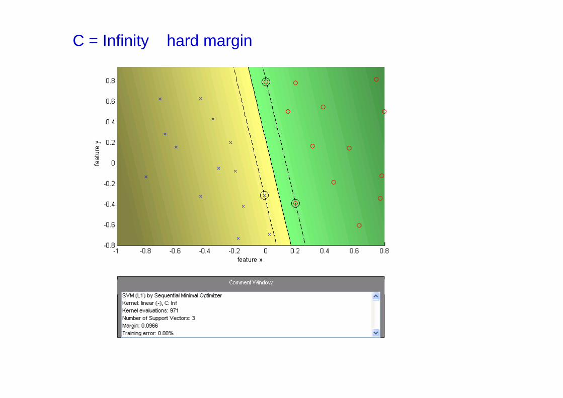
C = Infinity hard margin

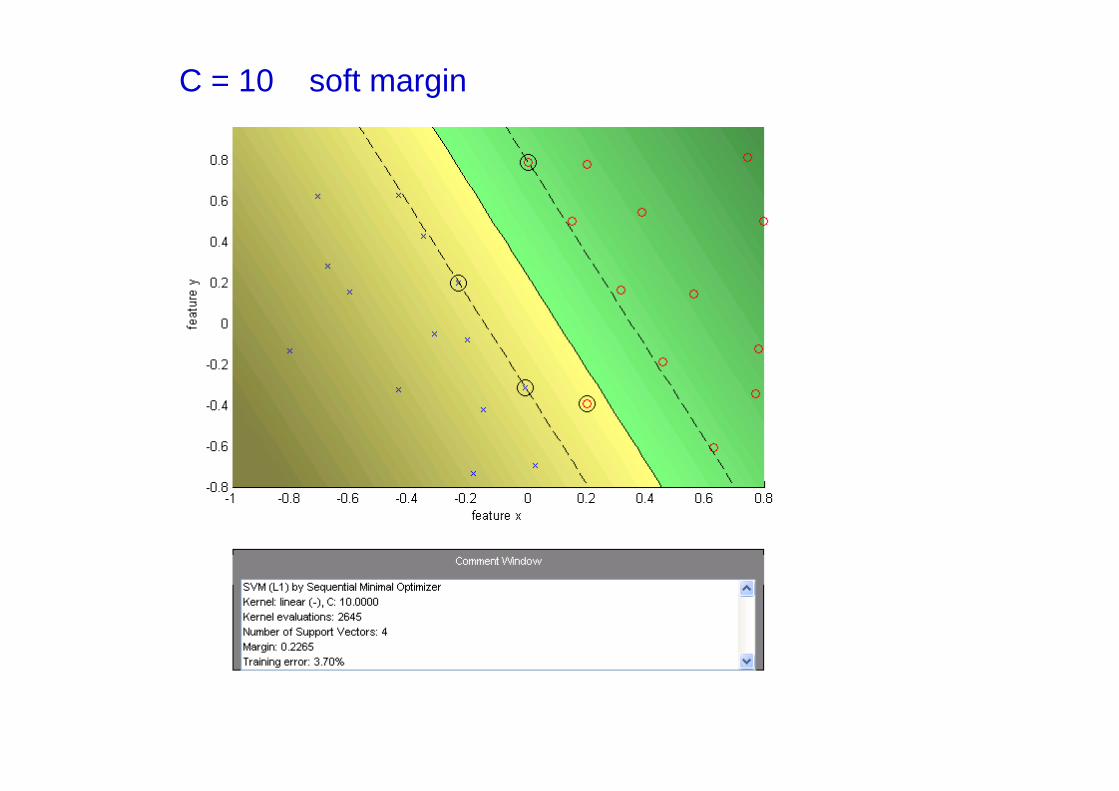
C = 10 soft margin

Application: Pedestrian detection in Computer Vision

Objective: detect (localize) standing humans in an image• cf face detection with a sliding window classifier

• reduces object detection to binary classification

• does an image window contain a person or not?

Method: the HOG detector

• Positive data – 1208 positive window examples

• Negative data – 1218 negative window examples (initially)

Training data and features

Feature: histogram of oriented gradients (HOG)

Feature vector dimension = 16 x 8 (for tiling) x 8 (orientations) = 1024

imagedominant direction HOG

frequ

ency

orientation

• tile window into 8 x 8 pixel cells

• each cell represented by HOG

Averaged positive examples

Training (Learning)• Represent each example window by a HOG feature vector

• Train a SVM classifier

Testing (Detection)

• Sliding window classifier

Algorithm

f(x) = w>x+ b

xi ∈ Rd, with d = 1024

Dalal and Triggs, CVPR 2005

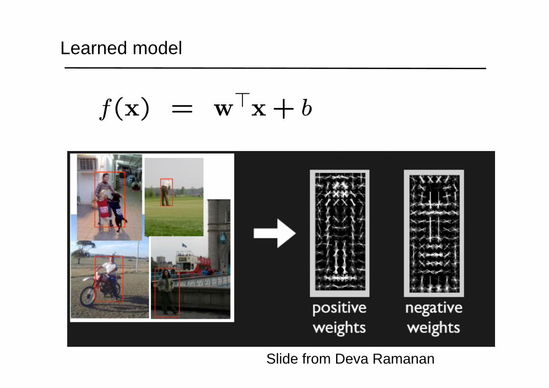
Learned model

Slide from Deva Ramanan

f(x) = w>x+ b

Slide from Deva Ramanan

OptimizationLearning an SVM has been formulated as a constrained optimization prob-

lem over w and ξ

minw∈Rd,ξi∈R+

||w||2 + CNXi

ξi subject to yi³w>xi+ b

´≥ 1− ξi for i = 1 . . . N

The constraint yi³w>xi+ b

´≥ 1− ξi, can be written more concisely as

yif(xi) ≥ 1− ξi

which, together with ξi ≥ 0, is equivalent to

ξi = max (0,1− yif(xi))Hence the learning problem is equivalent to the unconstrained optimiza-

tion problem over w

minw∈Rd

||w||2 + CNXi

max (0,1− yif(xi))

loss functionregularization

Loss function

w

Support Vector

Support Vector

wTx + b = 0

minw∈Rd

||w||2 + CNXi

max (0,1− yif(xi))

Points are in three categories:

1. yif(xi) > 1

Point is outside margin.

No contribution to loss

2. yif(xi) = 1

Point is on margin.

No contribution to loss.

As in hard margin case.

3. yif(xi) < 1

Point violates margin constraint.

Contributes to loss

loss function

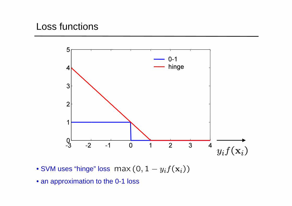
Loss functions

• SVM uses “hinge” loss

• an approximation to the 0-1 loss

max (0,1− yif(xi))

yif(xi)

minw∈Rd

CNXi

max (0,1− yif(xi)) + ||w||2

• Does this cost function have a unique solution?

• Does the solution depend on the starting point of an iterative optimization algorithm (such as gradient descent)?

local minimum

global minimum

If the cost function is convex, then a locally optimal point is globally optimal (provided the optimization is over a convex set, which it is in our case)

Optimization continued

Convex functions

Convex function examples

convex Not convex

A non-negative sum of convex functions is convex

SVM

minw∈Rd

CNXi

max (0,1− yif(xi)) + ||w||2

+

convex

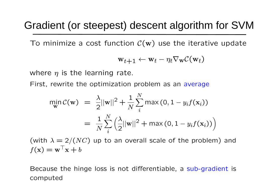
Gradient (or steepest) descent algorithm for SVM

First, rewrite the optimization problem as an average

minwC(w) =

λ

2||w||2 + 1

N

NXi

max (0,1− yif(xi))

=1

N

NXi

µλ

2||w||2 +max (0,1− yif(xi))

¶(with λ = 2/(NC) up to an overall scale of the problem) and

f(x) = w>x+ b

Because the hinge loss is not differentiable, a sub-gradient is

computed

To minimize a cost function C(w) use the iterative update

wt+1 ← wt − ηt∇wC(wt)where η is the learning rate.

Sub-gradient for hinge loss

L(xi, yi;w) = max (0,1− yif(xi)) f(xi) = w>xi+ b

yif(xi)

∂L∂w

= −yixi

∂L∂w

= 0

Sub-gradient descent algorithm for SVM

C(w) = 1

N

NXi

µλ

2||w||2 + L(xi, yi;w)

¶

The iterative update is

wt+1 ← wt − η∇wtC(wt)

← wt − η1

N

NXi

(λwt+∇wL(xi, yi;wt))

where η is the learning rate.

Then each iteration t involves cycling through the training data with the

updates:

wt+1 ← wt − η(λwt − yixi) if yif(xi) < 1

← wt − ηλwt otherwise

In the Pegasos algorithm the learning rate is set at ηt =1λt

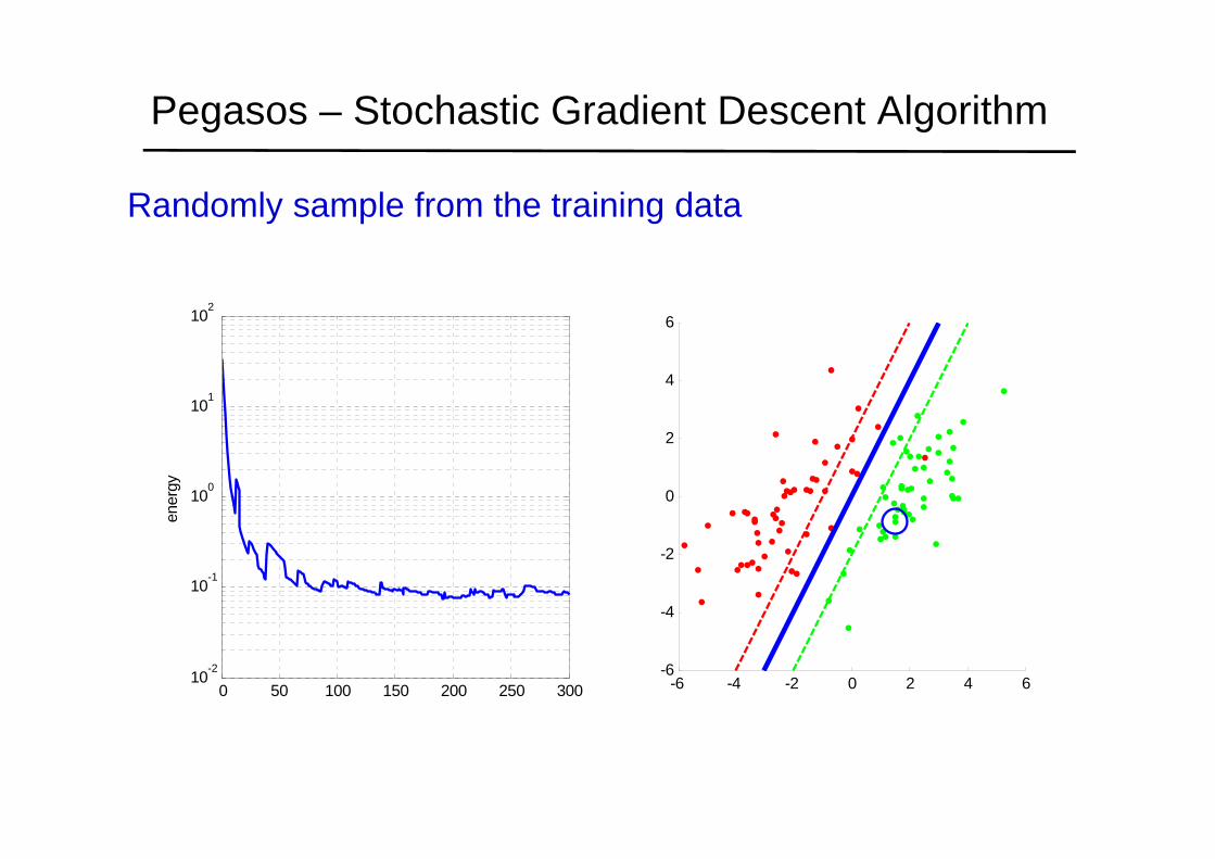
Pegasos – Stochastic Gradient Descent Algorithm

Randomly sample from the training data

0 50 100 150 200 250 30010-2

10-1

100

101

102

ener

gy

-6 -4 -2 0 2 4 6-6

-4

-2

0

2

4

6

Background reading and more …

• Next lecture – see that the SVM can be expressed as a sum over the support vectors:

• On web page: http://www.robots.ox.ac.uk/~az/lectures/ml

• links to SVM tutorials and video lectures

• MATLAB SVM demo

f(x) =Xi

αiyi(xi>x) + b

support vectors