lecture 24: partial correlation, multiple regression, and correlation … · 2017-12-11 · chapter...
TRANSCRIPT
Lecture 24:Partial correlation, multiple regression, and correlation
Ernesto F. L. Amaral
November 21, 2017Advanced Methods of Social Research (SOCI 420)
Source: Healey, Joseph F. 2015. ”Statistics: A Tool for Social Research.” Stamford: Cengage Learning. 10th edition. Chapter 15 (pp. 405–441).
Chapter learning objectives• Compute and interpret partial correlation
coefficients• Find and interpret the least-squares multiple
regression equation with partial slopes• Find and interpret standardized partial slopes or
beta-weights (b*)• Calculate and interpret the coefficient of multiple
determination (R2)• Explain the limitations of partial and regression
analysis
2
Multiple regression• Discuss ordinary least squares (OLS) multiple
regressions– OLS: linear regression– Multiple: at least two independent variables
• Disentangle and examine the separate effects of the independent variables
• Use all of the independent variables to predict Y• Assess the combined effects of the independent
variables on Y
3
Partial correlation• Partial correlation measures the correlation
between X and Y, controlling for Z
• Comparing the bivariate (zero-order) correlation to the partial (first-order) correlation– Allows us to determine if the relationship between X
and Y is direct, spurious, or intervening
– Interaction cannot be determined with partial correlations
4
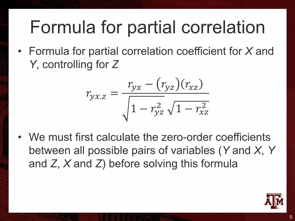
Formula for partial correlation• Formula for partial correlation coefficient for X and
Y, controlling for Z
• We must first calculate the zero-order coefficients between all possible pairs of variables (Y and X, Yand Z, X and Z) before solving this formula
5
𝑟"#.% =𝑟"# − 𝑟"% 𝑟#%
1 − 𝑟"%)� 1 − 𝑟#%)
�
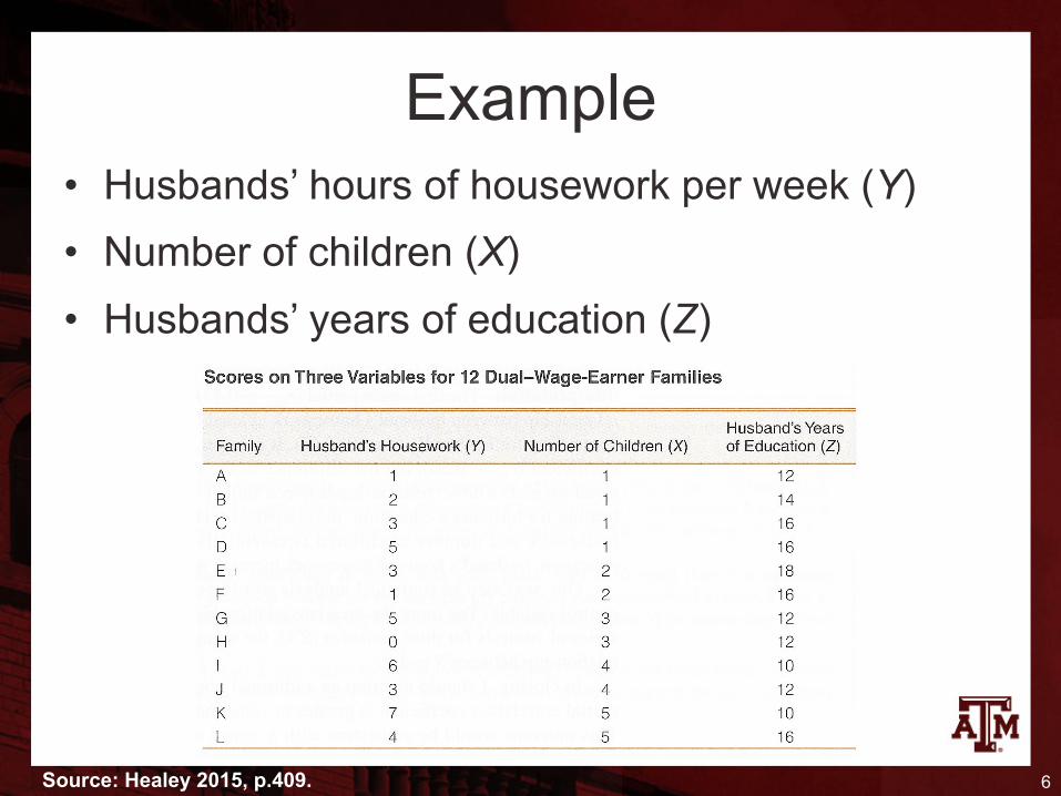
Example• Husbands’ hours of housework per week (Y)• Number of children (X)• Husbands’ years of education (Z)
6Source: Healey 2015, p.409.
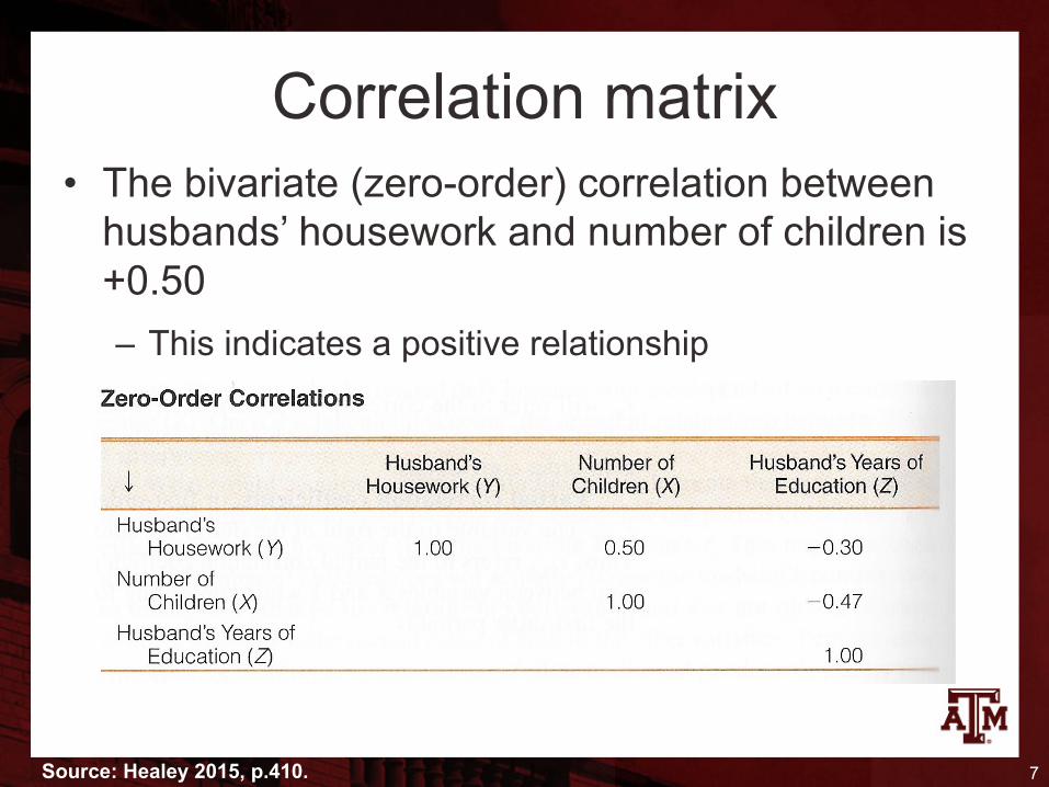
Correlation matrix• The bivariate (zero-order) correlation between
husbands’ housework and number of children is +0.50– This indicates a positive relationship
7Source: Healey 2015, p.410.
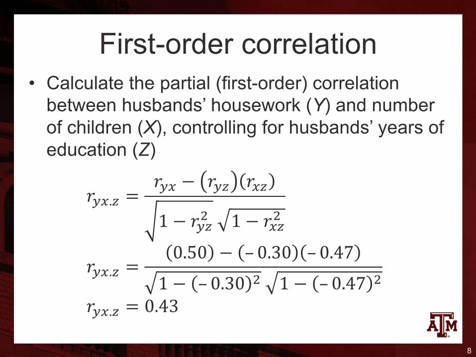
First-order correlation• Calculate the partial (first-order) correlation
between husbands’ housework (Y) and number of children (X), controlling for husbands’ years of education (Z)
8
𝑟"#.% =𝑟"# − 𝑟"% 𝑟#%
1 − 𝑟"%)� 1 − 𝑟#%)
�
𝑟"#.% =0.50 − –0.30 – 0.47
1 − –0.30 )� 1 − – 0.47 )�
𝑟"#.% = 0.43
Interpretation• Comparing the bivariate correlation (+0.50) to
the partial correlation (+0.43) finds little change
• The relationship between number of children and husbands’ housework has not changed, controlling for husbands’ education
• Therefore, we have evidence of a direct relationship
9
Bivariate & multiple regressions• Bivariate regression equation
Y = a + bX = β0 + β1X– a = β0 = Y intercept– b = β1 = slope
• Multivariate regression equationY = a + b1X1 + b2X2 = β0 + β1X1 + β2X2
– b1 = β1 = partial slope of the linear relationship between the first independent variable and Y
– b2 = β1 = partial slope of the linear relationship between the second independent variable and Y
10
Multiple regressionY = a + b1X1 + b2X2 = β0 + β1X1 + β2X2
• a = β0 = the Y intercept, where the regression line crosses the Y axis
• b1 = β1 = partial slope for X1 on Y– β1 indicates the change in Y for one unit change in X1,
controlling for X2
• b2 = β2 = partial slope for X2 on Y– β2 indicates the change in Y for one unit change in X2,
controlling for X1
11
Partial slopes• The partial slopes indicate the effect of each
independent variable on Y
• While controlling for the effect of the other independent variables
• This control is called ceteris paribus– Other things equal– Other things held constant
– All other things being equal12
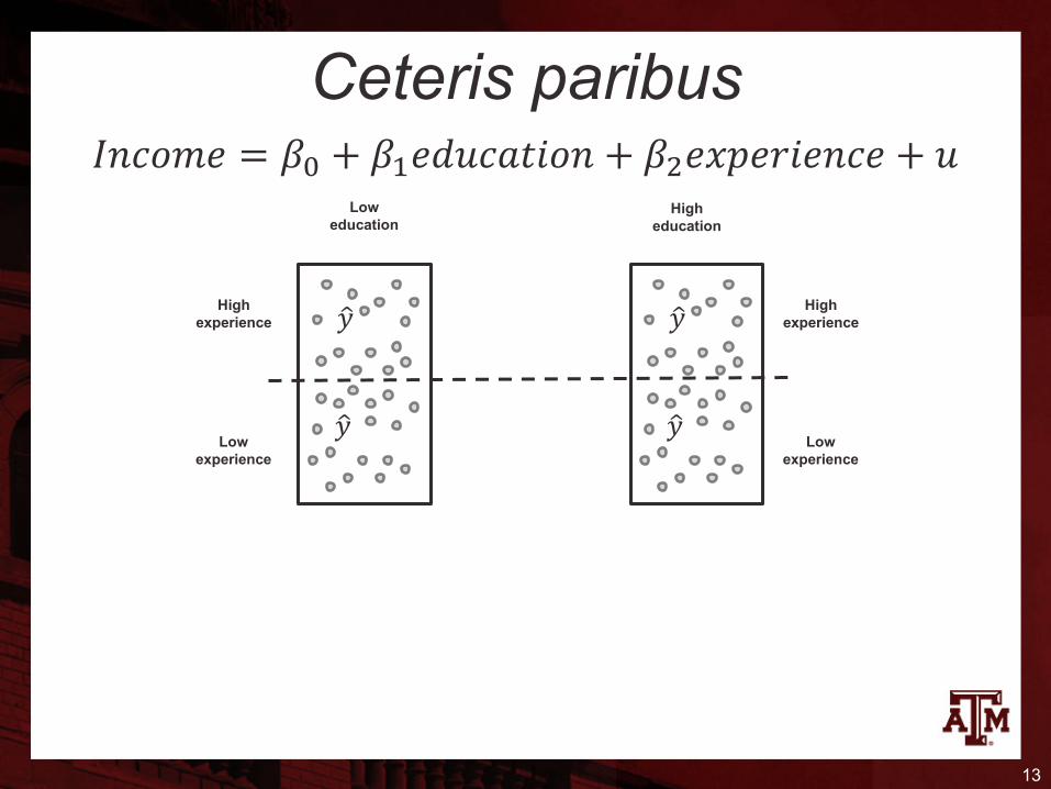
Ceteris paribus
13
Highexperience
Lowexperience
Loweducation
Higheducation
𝑦3
𝑦3
Highexperience
Lowexperience
𝑦3
𝑦3
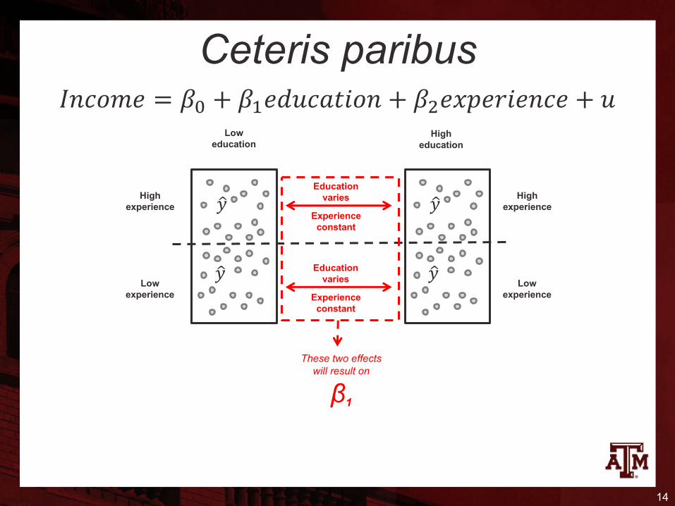
𝐼𝑛𝑐𝑜𝑚𝑒 = 𝛽; + 𝛽=𝑒𝑑𝑢𝑐𝑎𝑡𝑖𝑜𝑛 + 𝛽)𝑒𝑥𝑝𝑒𝑟𝑖𝑒𝑛𝑐𝑒 + 𝑢
Ceteris paribus
14
Highexperience
Lowexperience
Loweducation
Higheducation
𝑦3
𝑦3
Highexperience
Lowexperience
𝑦3
𝑦3
Experienceconstant
Educationvaries
Experienceconstant
Educationvaries
These two effectswill result on
β1
𝐼𝑛𝑐𝑜𝑚𝑒 = 𝛽; + 𝛽=𝑒𝑑𝑢𝑐𝑎𝑡𝑖𝑜𝑛 + 𝛽)𝑒𝑥𝑝𝑒𝑟𝑖𝑒𝑛𝑐𝑒 + 𝑢
Ceteris paribus
15
Highexperience
Lowexperience
Loweducation
Higheducation
𝑦3
𝑦3
Highexperience
Lowexperience
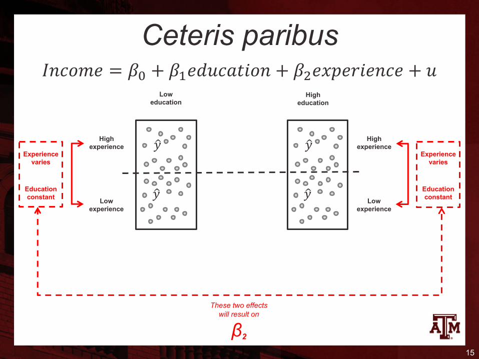
Educationconstant
Experiencevaries
Educationconstant
Experiencevaries
These two effectswill result on
β2
𝑦3
𝑦3
𝐼𝑛𝑐𝑜𝑚𝑒 = 𝛽; + 𝛽=𝑒𝑑𝑢𝑐𝑎𝑡𝑖𝑜𝑛 + 𝛽)𝑒𝑥𝑝𝑒𝑟𝑖𝑒𝑛𝑐𝑒 + 𝑢
Ceteris paribus
16
Highexperience
Lowexperience
Loweducation
Higheducation
𝑦3
𝑦3
Highexperience
Lowexperience
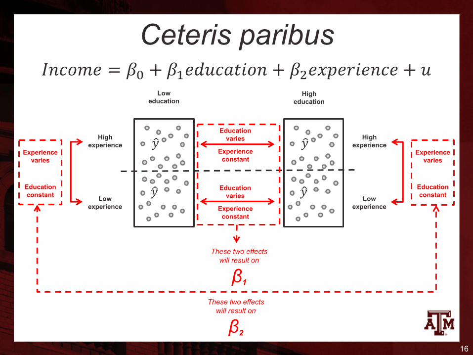
Educationconstant
Experiencevaries
Educationconstant
Experiencevaries
These two effectswill result on
β2
𝑦3
𝑦3
Experienceconstant
Educationvaries
Experienceconstant
Educationvaries
These two effectswill result on
β1
𝐼𝑛𝑐𝑜𝑚𝑒 = 𝛽; + 𝛽=𝑒𝑑𝑢𝑐𝑎𝑡𝑖𝑜𝑛 + 𝛽)𝑒𝑥𝑝𝑒𝑟𝑖𝑒𝑛𝑐𝑒 + 𝑢
• The partial slopes show the effects of the X’s in their original units
• These values can be used to predict scores on Y
• Partial slopes must be computed before computing the Y intercept (β0)
Interpretation of partial slopes
17
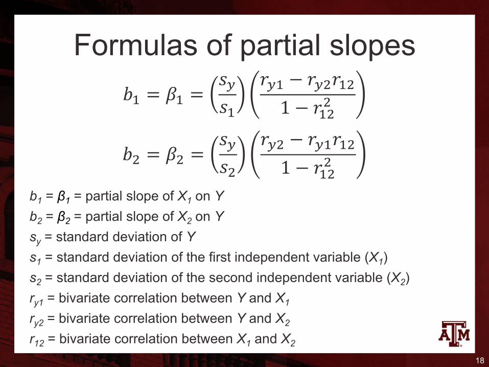
Formulas of partial slopes
18
b1 = β1 = partial slope of X1 on Yb2 = β2 = partial slope of X2 on Ysy = standard deviation of Ys1 = standard deviation of the first independent variable (X1)s2 = standard deviation of the second independent variable (X2)ry1 = bivariate correlation between Y and X1
ry2 = bivariate correlation between Y and X2
r12 = bivariate correlation between X1 and X2
𝑏= = 𝛽= =𝑠"𝑠=
𝑟"= − 𝑟")𝑟=)1 − 𝑟=))
𝑏) = 𝛽) =𝑠"𝑠)
𝑟") − 𝑟"=𝑟=)1 − 𝑟=))
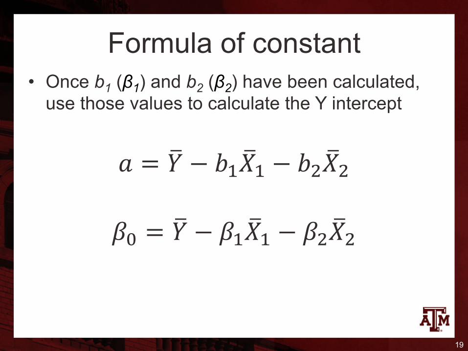
Formula of constant• Once b1 (β1) and b2 (β2) have been calculated,
use those values to calculate the Y intercept
19
𝑎 = 𝑌H − 𝑏=𝑋H= − 𝑏)𝑋H)
𝛽; = 𝑌H − 𝛽=𝑋H= − 𝛽)𝑋H)
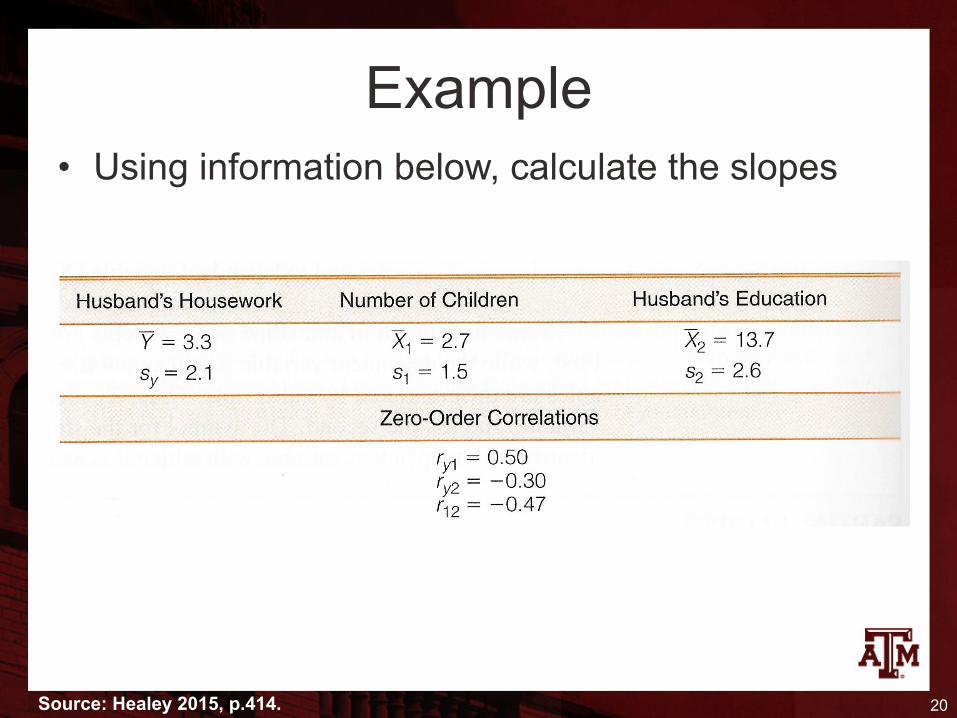
Example• Using information below, calculate the slopes
20Source: Healey 2015, p.414.
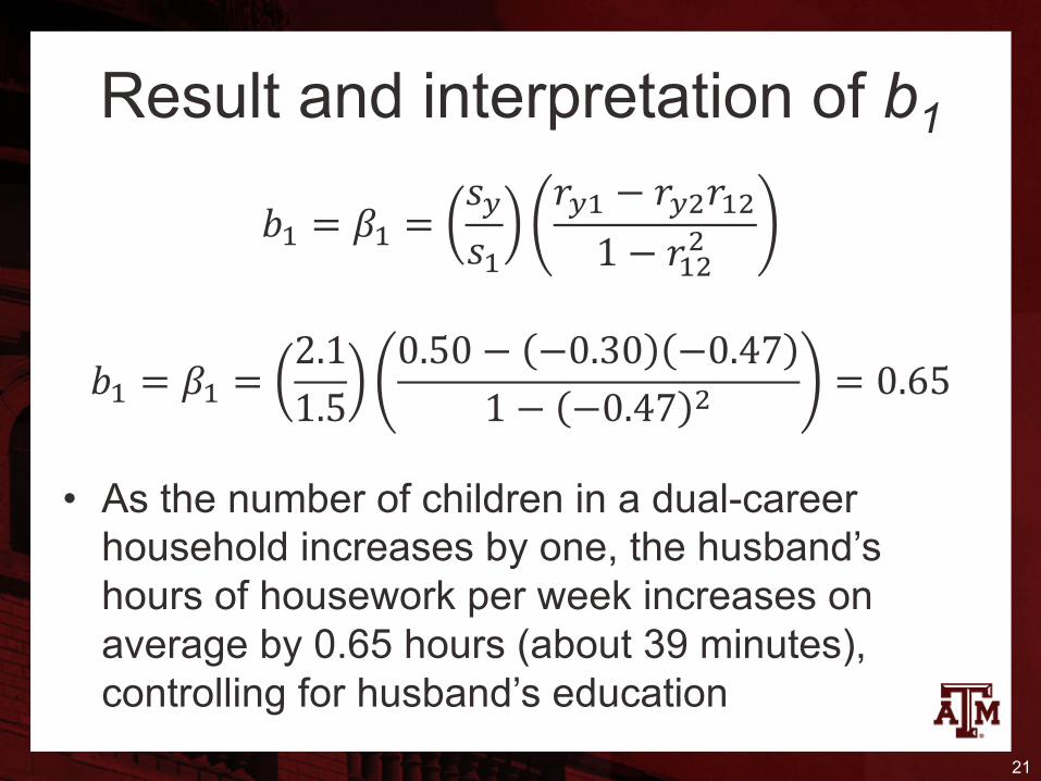
Result and interpretation of b1
• As the number of children in a dual-career household increases by one, the husband’s hours of housework per week increases on average by 0.65 hours (about 39 minutes), controlling for husband’s education
21
𝑏= = 𝛽= =𝑠"𝑠=
𝑟"= − 𝑟")𝑟=)1 − 𝑟=))
𝑏= = 𝛽= =2.11.5
0.50 − −0.30 −0.471 − −0.47 ) = 0.65
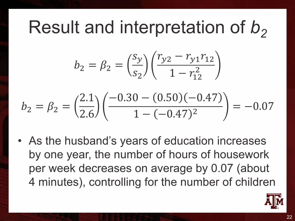
Result and interpretation of b2
• As the husband’s years of education increases by one year, the number of hours of housework per week decreases on average by 0.07 (about 4 minutes), controlling for the number of children
22
𝑏) = 𝛽) =𝑠"𝑠)
𝑟") − 𝑟"=𝑟=)1 − 𝑟=))
𝑏) = 𝛽) =2.12.6
−0.30 − 0.50 −0.471 − −0.47 ) = −0.07
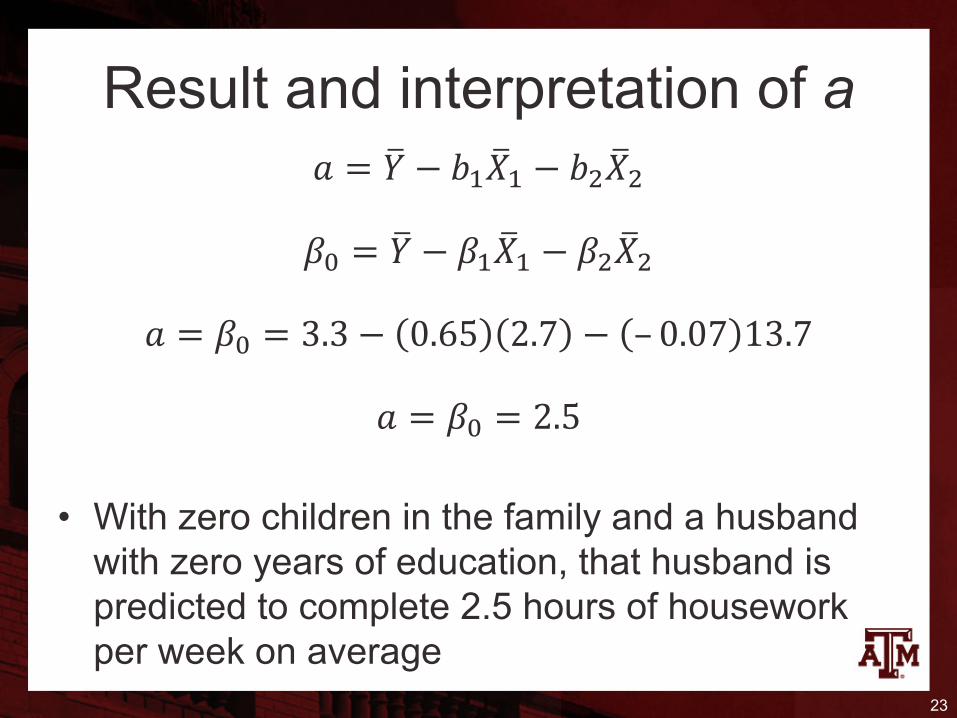
Result and interpretation of a𝑎 = 𝑌H − 𝑏=𝑋H= − 𝑏)𝑋H)
𝛽; = 𝑌H − 𝛽=𝑋H= − 𝛽)𝑋H)
𝑎 = 𝛽; = 3.3 − 0.65 2.7 − – 0.07 13.7
𝑎 = 𝛽; = 2.5
• With zero children in the family and a husband with zero years of education, that husband is predicted to complete 2.5 hours of housework per week on average
23
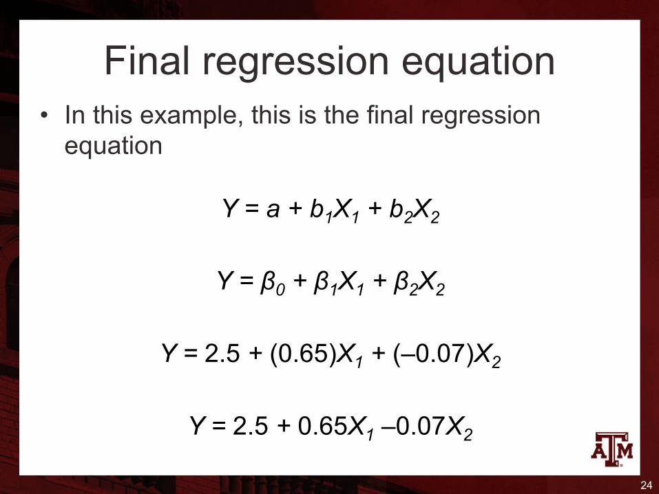
Final regression equation• In this example, this is the final regression
equation
Y = a + b1X1 + b2X2
Y = β0 + β1X1 + β2X2
Y = 2.5 + (0.65)X1 + (–0.07)X2
Y = 2.5 + 0.65X1 –0.07X2
24
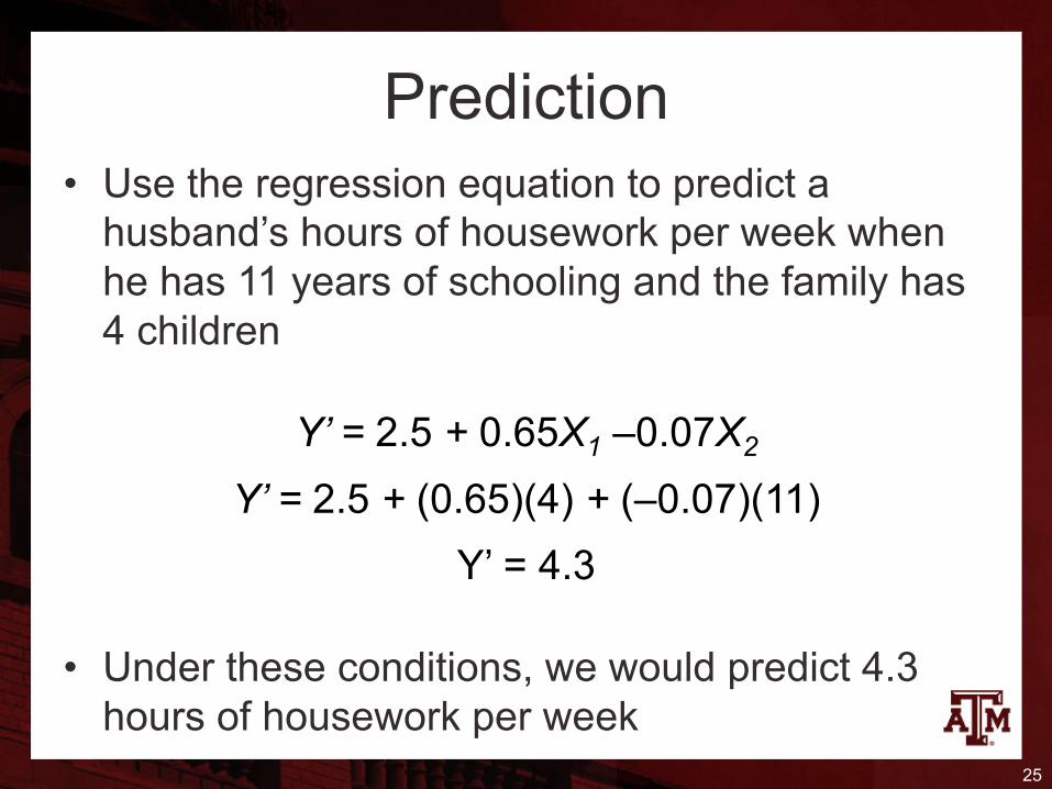
Prediction• Use the regression equation to predict a
husband’s hours of housework per week when he has 11 years of schooling and the family has 4 children
Y’ = 2.5 + 0.65X1 –0.07X2
Y’ = 2.5 + (0.65)(4) + (–0.07)(11)Y’ = 4.3
• Under these conditions, we would predict 4.3 hours of housework per week
25
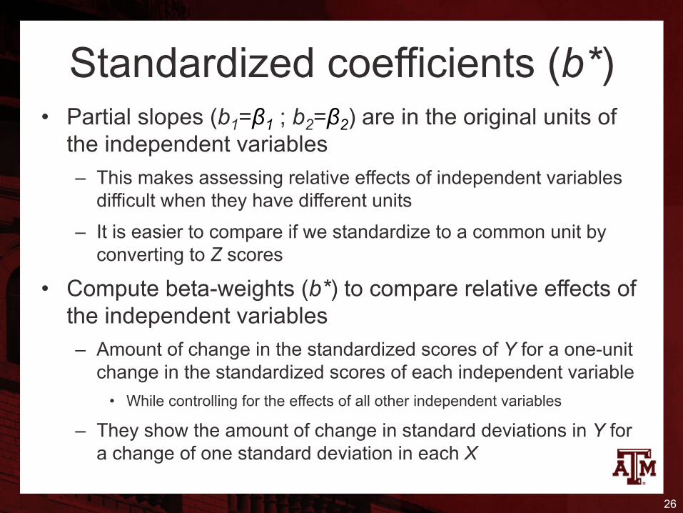
Standardized coefficients (b*)• Partial slopes (b1=β1 ; b2=β2) are in the original units of
the independent variables– This makes assessing relative effects of independent variables
difficult when they have different units– It is easier to compare if we standardize to a common unit by
converting to Z scores
• Compute beta-weights (b*) to compare relative effects of the independent variables– Amount of change in the standardized scores of Y for a one-unit
change in the standardized scores of each independent variable• While controlling for the effects of all other independent variables
– They show the amount of change in standard deviations in Y for a change of one standard deviation in each X
26
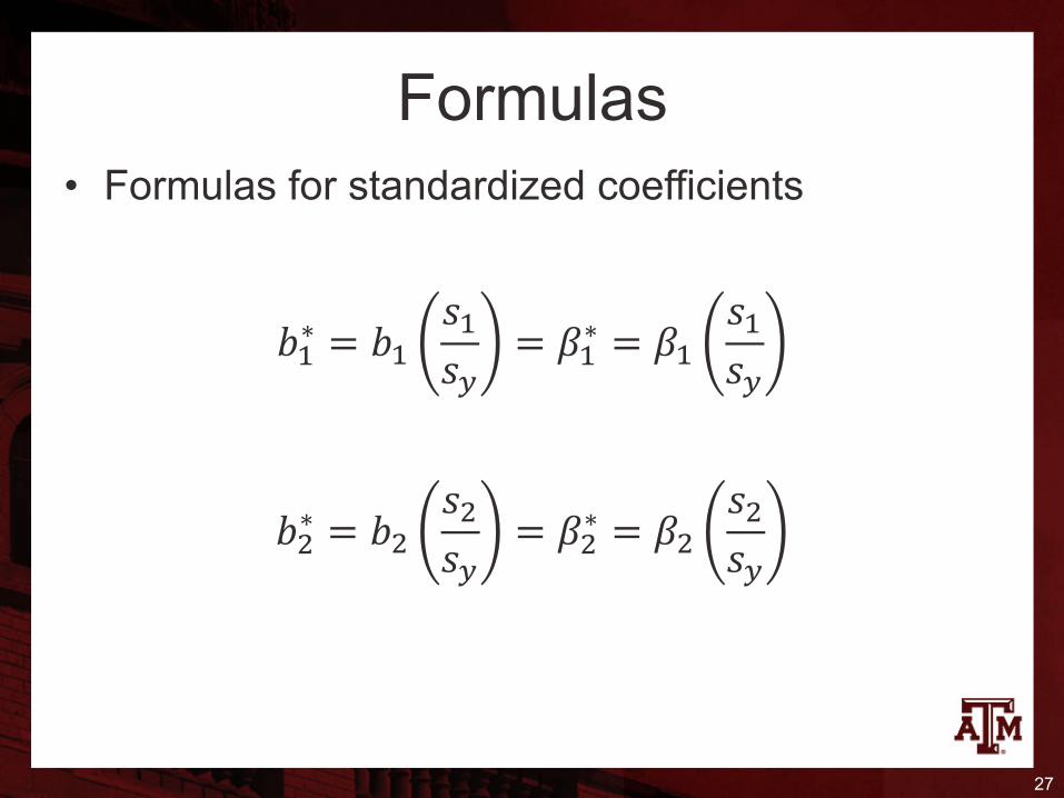
Formulas• Formulas for standardized coefficients
𝑏=∗ = 𝑏=𝑠=𝑠"
= 𝛽=∗ = 𝛽=𝑠=𝑠"
𝑏)∗ = 𝑏)𝑠)𝑠"
= 𝛽)∗ = 𝛽)𝑠)𝑠"
27
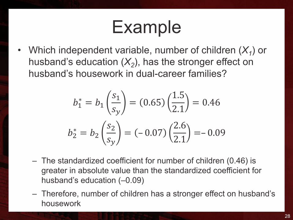
Example• Which independent variable, number of children (X1) or
husband’s education (X2), has the stronger effect on husband’s housework in dual-career families?
𝑏=∗ = 𝑏=𝑠=𝑠"
= 0.651.52.1
= 0.46
𝑏)∗ = 𝑏)𝑠)𝑠"
= – 0.072.62.1
=– 0.09
– The standardized coefficient for number of children (0.46) is greater in absolute value than the standardized coefficient for husband’s education (–0.09)
– Therefore, number of children has a stronger effect on husband’s housework
28
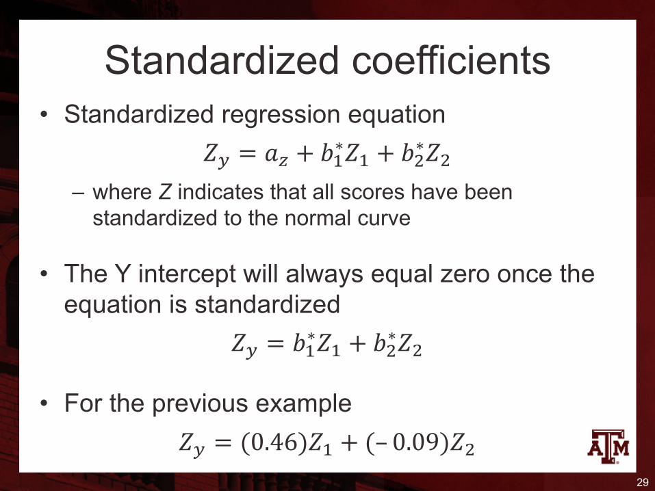
Standardized coefficients• Standardized regression equation
𝑍" = 𝑎% + 𝑏=∗𝑍= + 𝑏)∗𝑍)– where Z indicates that all scores have been
standardized to the normal curve
• The Y intercept will always equal zero once the equation is standardized
𝑍" = 𝑏=∗𝑍= + 𝑏)∗𝑍)
• For the previous example𝑍" = (0.46)𝑍= + (– 0.09)𝑍)
29
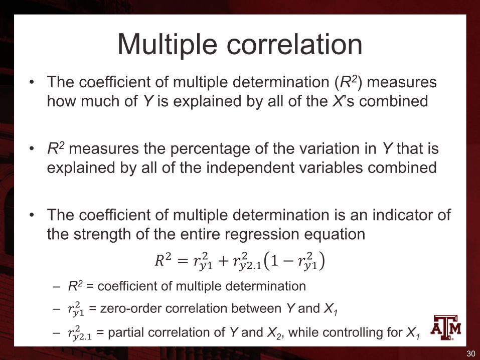
Multiple correlation• The coefficient of multiple determination (R2) measures
how much of Y is explained by all of the X’s combined
• R2 measures the percentage of the variation in Y that is explained by all of the independent variables combined
• The coefficient of multiple determination is an indicator of the strength of the entire regression equation
𝑅) = 𝑟"=) + 𝑟").=) 1 − 𝑟"=)
– R2 = coefficient of multiple determination– 𝑟"=) = zero-order correlation between Y and X1
– 𝑟").=) = partial correlation of Y and X2, while controlling for X1
30
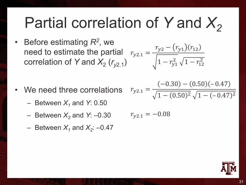
Partial correlation of Y and X2• Before estimating R2, we
need to estimate the partial correlation of Y and X2 (ry2.1)
• We need three correlations– Between X1 and Y: 0.50
– Between X2 and Y: –0.30
– Between X1 and X2: –0.47
31
𝑟").= =𝑟") − 𝑟"= 𝑟=)
1 − 𝑟"=)� 1 − 𝑟=))
�
𝑟").= =−0.30 − 0.50 – 0.47
1 − 0.50 )� 1 − – 0.47 )�
𝑟").= = −0.08
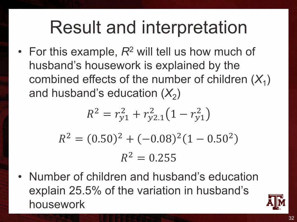
Result and interpretation• For this example, R2 will tell us how much of
husband’s housework is explained by the combined effects of the number of children (X1) and husband’s education (X2)
• Number of children and husband’s education explain 25.5% of the variation in husband’s housework
32
𝑅) = 𝑟"=) + 𝑟").=) 1 − 𝑟"=)
𝑅) = 0.50 ) + −0.08 ) 1 − 0.50)
𝑅) = 0.255
Normality assumption• OLS regressions require normal distribution for
its interval-ratio-level variables
• We can analyze histograms to determine if variables have a normal distribution
33
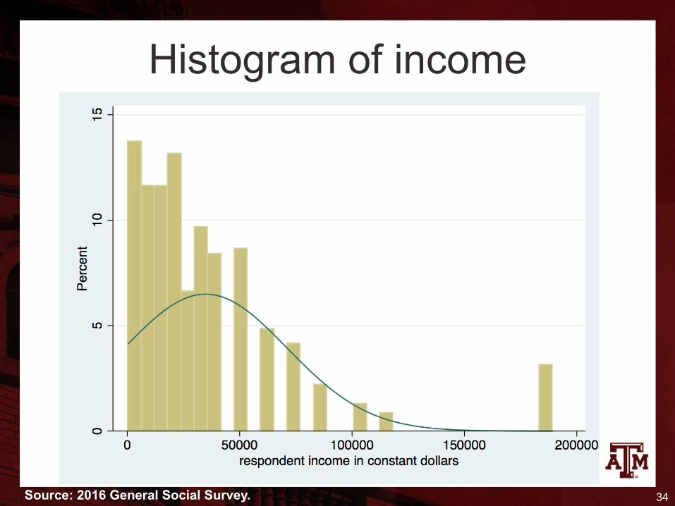
Histogram of income
34Source: 2016 General Social Survey.
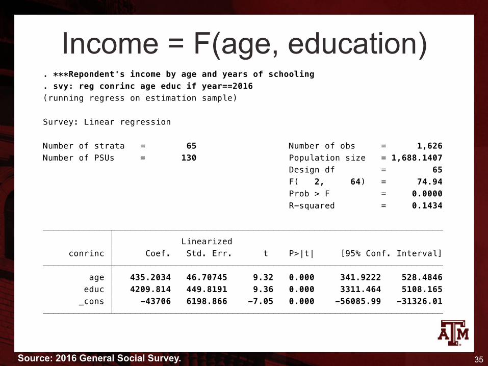
Income = F(age, education)
35
.
_cons -43706 6198.866 -7.05 0.000 -56085.99 -31326.01 educ 4209.814 449.8191 9.36 0.000 3311.464 5108.165 age 435.2034 46.70745 9.32 0.000 341.9222 528.4846 conrinc Coef. Std. Err. t P>|t| [95% Conf. Interval] Linearized
R-squared = 0.1434 Prob > F = 0.0000 F( 2, 64) = 74.94 Design df = 65Number of PSUs = 130 Population size = 1,688.1407Number of strata = 65 Number of obs = 1,626
Survey: Linear regression
(running regress on estimation sample). svy: reg conrinc age educ if year==2016. ***Repondent's income by age and years of schooling
Source: 2016 General Social Survey.
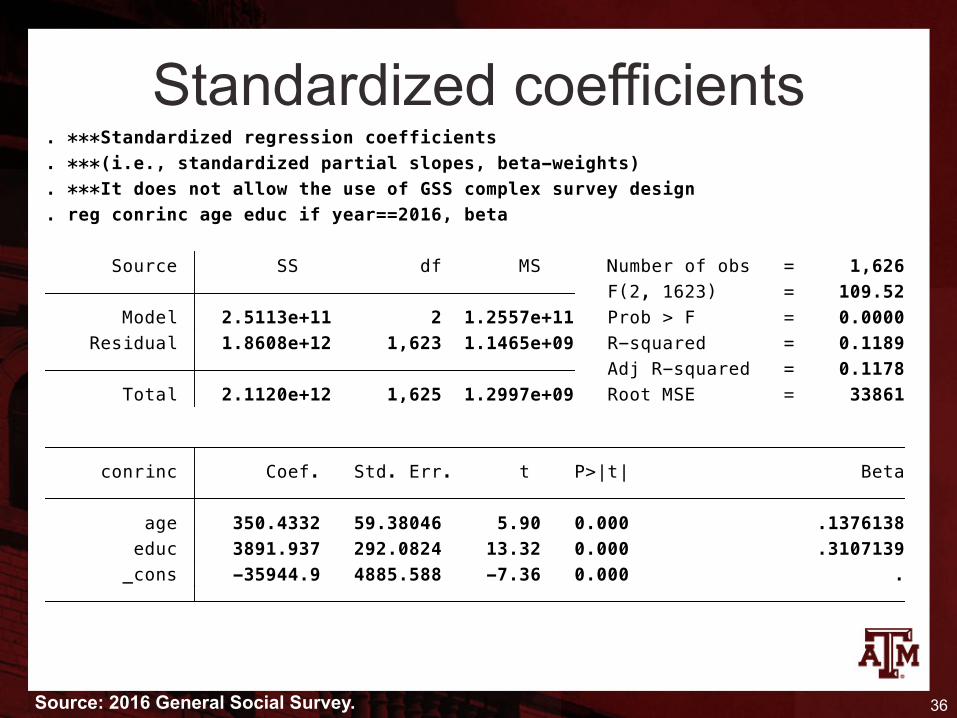
Standardized coefficients
36Source: 2016 General Social Survey.
_cons -35944.9 4885.588 -7.36 0.000 . educ 3891.937 292.0824 13.32 0.000 .3107139 age 350.4332 59.38046 5.90 0.000 .1376138 conrinc Coef. Std. Err. t P>|t| Beta
Total 2.1120e+12 1,625 1.2997e+09 Root MSE = 33861 Adj R-squared = 0.1178 Residual 1.8608e+12 1,623 1.1465e+09 R-squared = 0.1189 Model 2.5113e+11 2 1.2557e+11 Prob > F = 0.0000 F(2, 1623) = 109.52 Source SS df MS Number of obs = 1,626
. reg conrinc age educ if year==2016, beta
. ***It does not allow the use of GSS complex survey design
. ***(i.e., standardized partial slopes, beta-weights)
. ***Standardized regression coefficients
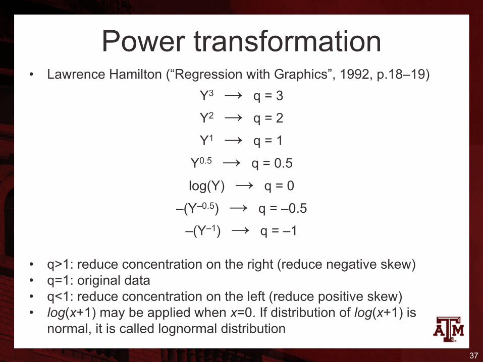
Power transformation• Lawrence Hamilton (“Regression with Graphics”, 1992, p.18–19)
Y3 → q = 3Y2 → q = 2Y1 → q = 1
Y0.5 → q = 0.5log(Y) → q = 0
–(Y–0.5) → q = –0.5–(Y–1) → q = –1
• q>1: reduce concentration on the right (reduce negative skew)• q=1: original data• q<1: reduce concentration on the left (reduce positive skew)• log(x+1) may be applied when x=0. If distribution of log(x+1) is
normal, it is called lognormal distribution
37
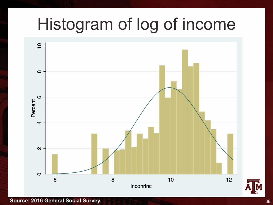
Histogram of log of income
38Source: 2016 General Social Survey.
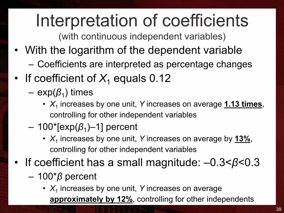
Interpretation of coefficients(with continuous independent variables)
• With the logarithm of the dependent variable– Coefficients are interpreted as percentage changes
• If coefficient of X1 equals 0.12– exp(β1) times
• X1 increases by one unit, Y increases on average 1.13 times, controlling for other independent variables
– 100*[exp(β1)–1] percent• X1 increases by one unit, Y increases on average by 13%,
controlling for other independent variables
• If coefficient has a small magnitude: –0.3<β<0.3– 100*β percent
• X1 increases by one unit, Y increases on average approximately by 12%, controlling for other independents
39
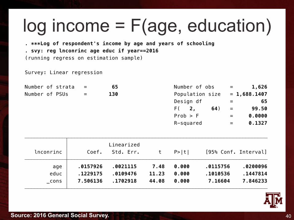
log income = F(age, education)
40Source: 2016 General Social Survey.
_cons 7.506136 .1702918 44.08 0.000 7.16604 7.846233 educ .1229175 .0109476 11.23 0.000 .1010536 .1447814 age .0157926 .0021115 7.48 0.000 .0115756 .0200096 lnconrinc Coef. Std. Err. t P>|t| [95% Conf. Interval] Linearized
R-squared = 0.1327 Prob > F = 0.0000 F( 2, 64) = 99.50 Design df = 65Number of PSUs = 130 Population size = 1,688.1407Number of strata = 65 Number of obs = 1,626
Survey: Linear regression
(running regress on estimation sample). svy: reg lnconrinc age educ if year==2016. ***Log of respondent's income by age and years of schooling
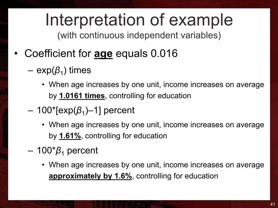
Interpretation of example(with continuous independent variables)
• Coefficient for age equals 0.016– exp(β1) times
• When age increases by one unit, income increases on average by 1.0161 times, controlling for education
– 100*[exp(β1)–1] percent• When age increases by one unit, income increases on average
by 1.61%, controlling for education
– 100*β1 percent• When age increases by one unit, income increases on average
approximately by 1.6%, controlling for education
41
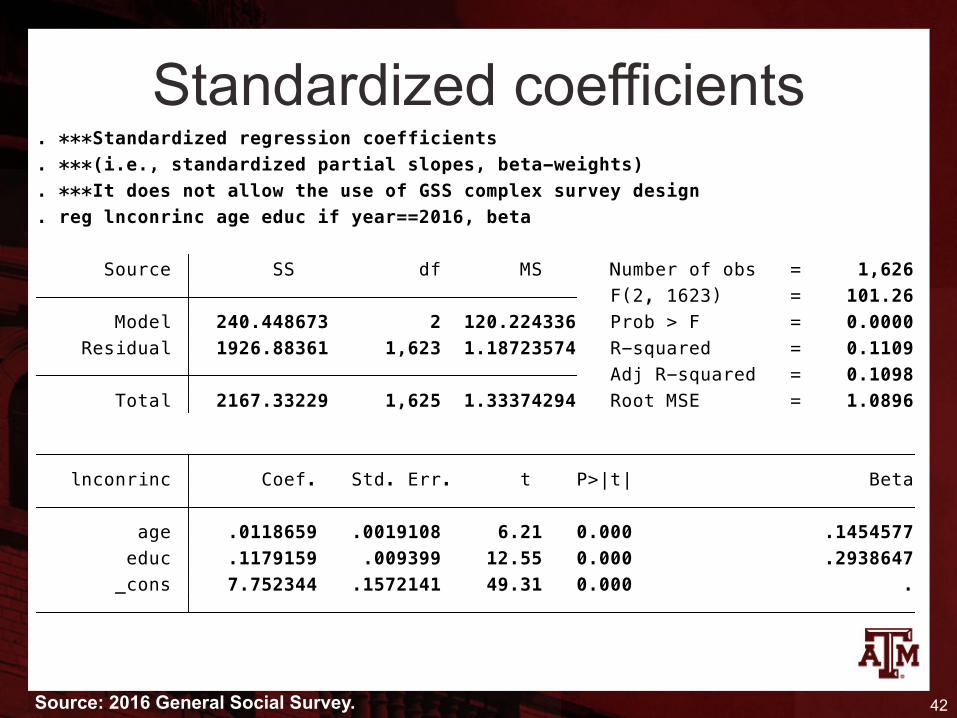
Standardized coefficients
42Source: 2016 General Social Survey.
_cons 7.752344 .1572141 49.31 0.000 . educ .1179159 .009399 12.55 0.000 .2938647 age .0118659 .0019108 6.21 0.000 .1454577 lnconrinc Coef. Std. Err. t P>|t| Beta
Total 2167.33229 1,625 1.33374294 Root MSE = 1.0896 Adj R-squared = 0.1098 Residual 1926.88361 1,623 1.18723574 R-squared = 0.1109 Model 240.448673 2 120.224336 Prob > F = 0.0000 F(2, 1623) = 101.26 Source SS df MS Number of obs = 1,626
. reg lnconrinc age educ if year==2016, beta
. ***It does not allow the use of GSS complex survey design
. ***(i.e., standardized partial slopes, beta-weights)
. ***Standardized regression coefficients
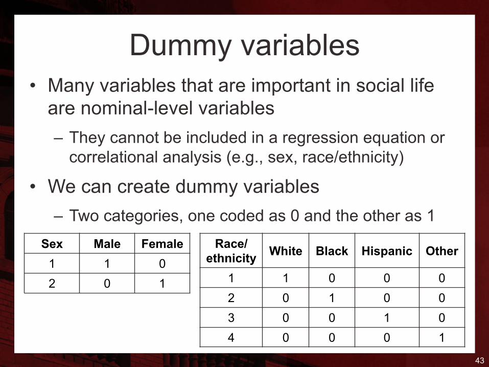
Dummy variables• Many variables that are important in social life
are nominal-level variables– They cannot be included in a regression equation or
correlational analysis (e.g., sex, race/ethnicity)
• We can create dummy variables– Two categories, one coded as 0 and the other as 1
43
Sex Male Female1 1 02 0 1
Race/ethnicity White Black Hispanic Other
1 1 0 0 02 0 1 0 03 0 0 1 04 0 0 0 1
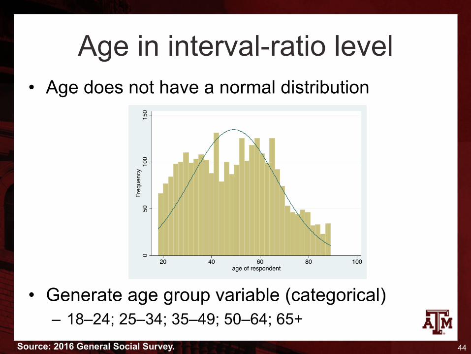
Age in interval-ratio level• Age does not have a normal distribution
• Generate age group variable (categorical)– 18–24; 25–34; 35–49; 50–64; 65+
44Source: 2016 General Social Survey.
050
100
150
Freq
uenc
y
20 40 60 80 100age of respondent
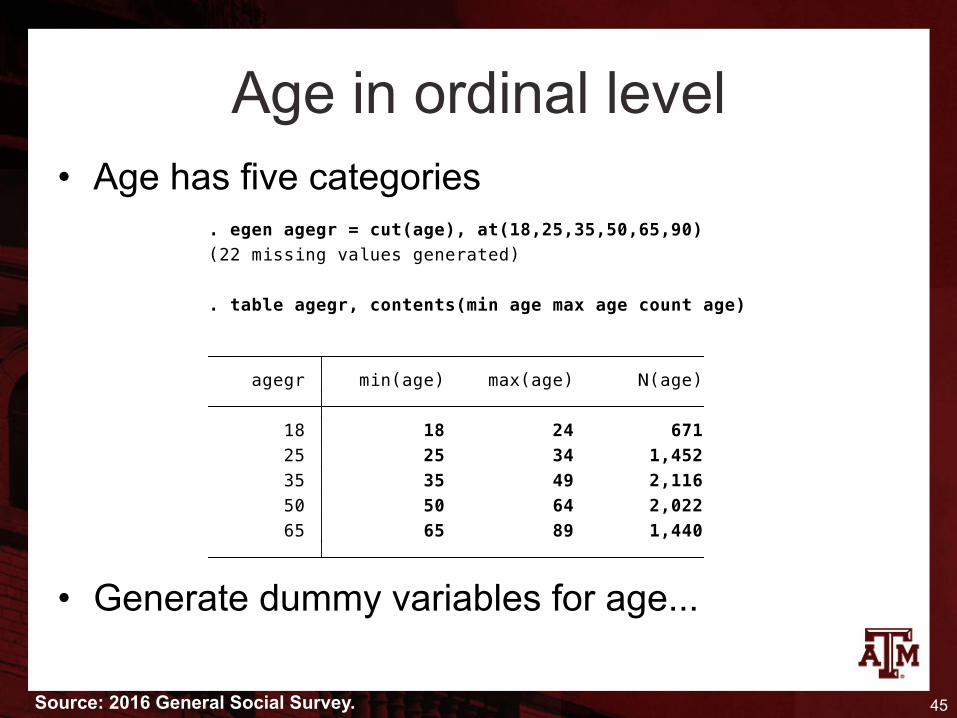
Age in ordinal level• Age has five categories
• Generate dummy variables for age...
45Source: 2016 General Social Survey.
65 65 89 1,440 50 50 64 2,022 35 35 49 2,116 25 25 34 1,452 18 18 24 671 agegr min(age) max(age) N(age)
. table agegr, contents(min age max age count age)
(22 missing values generated). egen agegr = cut(age), at(18,25,35,50,65,90)
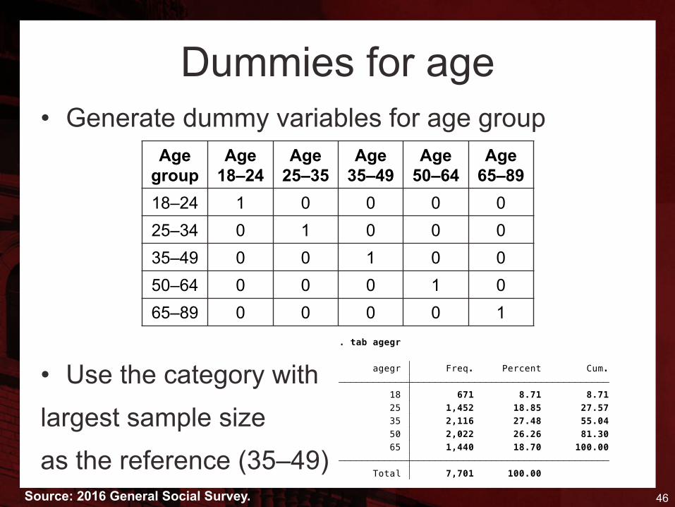
Dummies for age• Generate dummy variables for age group
• Use the category withlargest sample sizeas the reference (35–49)
46
Agegroup
Age18–24
Age25–35
Age35–49
Age50–64
Age65–89
18–24 1 0 0 0 025–34 0 1 0 0 035–49 0 0 1 0 050–64 0 0 0 1 065–89 0 0 0 0 1
.
Total 7,701 100.00 65 1,440 18.70 100.00 50 2,022 26.26 81.30 35 2,116 27.48 55.04 25 1,452 18.85 27.57 18 671 8.71 8.71 agegr Freq. Percent Cum.
. tab agegr
Source: 2016 General Social Survey.
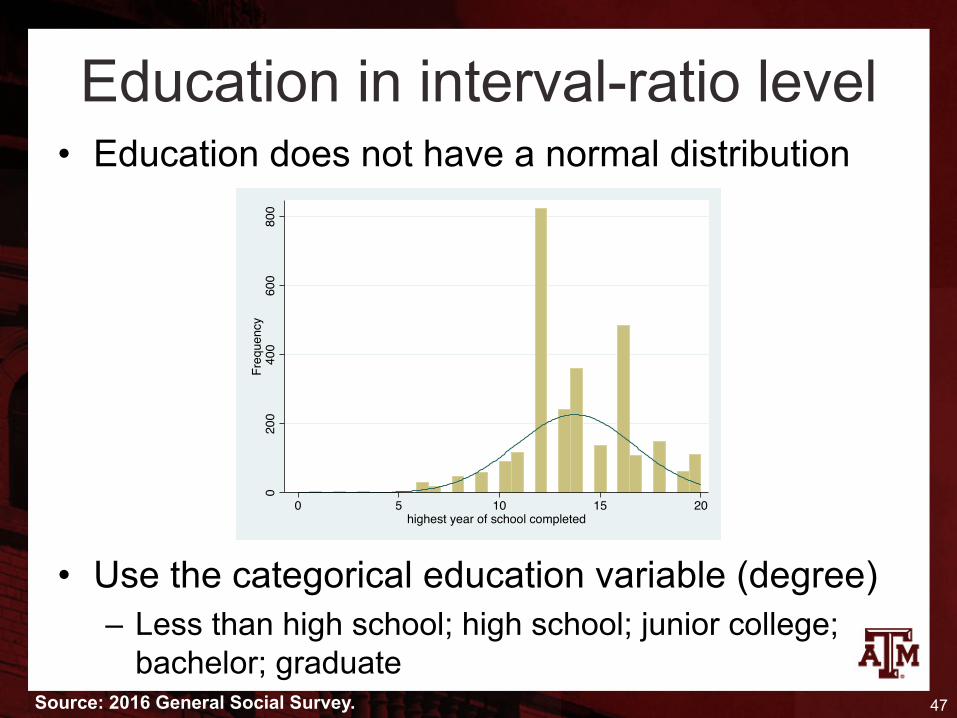
Education in interval-ratio level• Education does not have a normal distribution
• Use the categorical education variable (degree)– Less than high school; high school; junior college;
bachelor; graduate47Source: 2016 General Social Survey.
020
040
060
080
0Fr
eque
ncy
0 5 10 15 20highest year of school completed
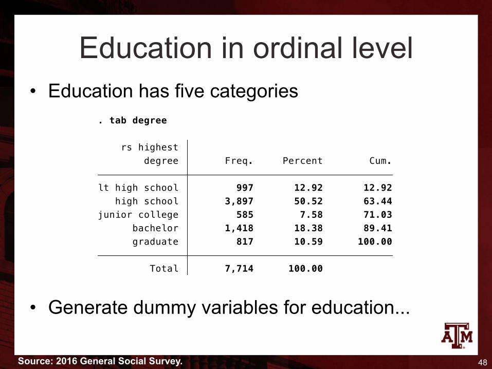
Education in ordinal level• Education has five categories
• Generate dummy variables for education...
48Source: 2016 General Social Survey.
.
Total 7,714 100.00 graduate 817 10.59 100.00 bachelor 1,418 18.38 89.41junior college 585 7.58 71.03 high school 3,897 50.52 63.44lt high school 997 12.92 12.92 degree Freq. Percent Cum. rs highest
. tab degree
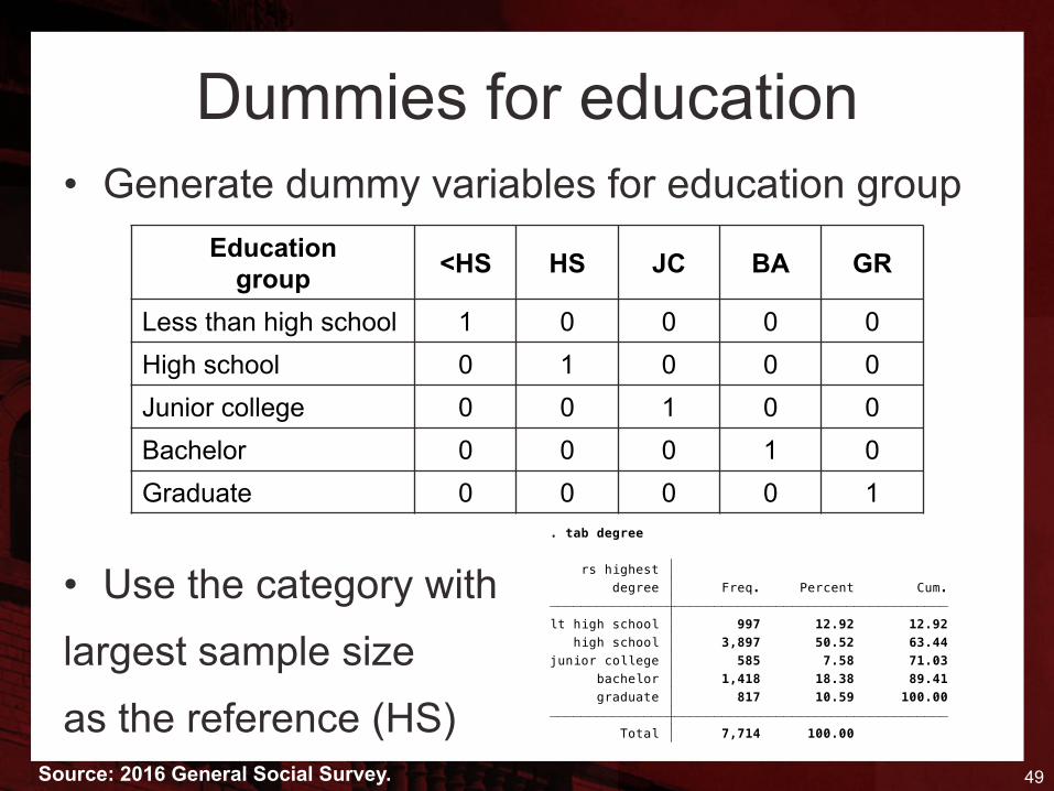
Dummies for education• Generate dummy variables for education group
• Use the category withlargest sample sizeas the reference (HS)
49
Educationgroup <HS HS JC BA GR
Less than high school 1 0 0 0 0High school 0 1 0 0 0Junior college 0 0 1 0 0Bachelor 0 0 0 1 0Graduate 0 0 0 0 1
Source: 2016 General Social Survey. .
Total 7,714 100.00 graduate 817 10.59 100.00 bachelor 1,418 18.38 89.41junior college 585 7.58 71.03 high school 3,897 50.52 63.44lt high school 997 12.92 12.92 degree Freq. Percent Cum. rs highest
. tab degree
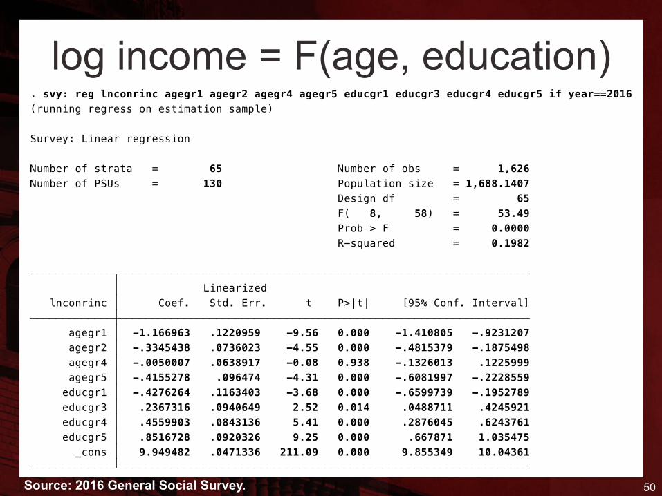
log income = F(age, education)
50Source: 2016 General Social Survey..
_cons 9.949482 .0471336 211.09 0.000 9.855349 10.04361 educgr5 .8516728 .0920326 9.25 0.000 .667871 1.035475 educgr4 .4559903 .0843136 5.41 0.000 .2876045 .6243761 educgr3 .2367316 .0940649 2.52 0.014 .0488711 .4245921 educgr1 -.4276264 .1163403 -3.68 0.000 -.6599739 -.1952789 agegr5 -.4155278 .096474 -4.31 0.000 -.6081997 -.2228559 agegr4 -.0050007 .0638917 -0.08 0.938 -.1326013 .1225999 agegr2 -.3345438 .0736023 -4.55 0.000 -.4815379 -.1875498 agegr1 -1.166963 .1220959 -9.56 0.000 -1.410805 -.9231207 lnconrinc Coef. Std. Err. t P>|t| [95% Conf. Interval] Linearized
R-squared = 0.1982 Prob > F = 0.0000 F( 8, 58) = 53.49 Design df = 65Number of PSUs = 130 Population size = 1,688.1407Number of strata = 65 Number of obs = 1,626
Survey: Linear regression
(running regress on estimation sample). svy: reg lnconrinc agegr1 agegr2 agegr4 agegr5 educgr1 educgr3 educgr4 educgr5 if year==2016
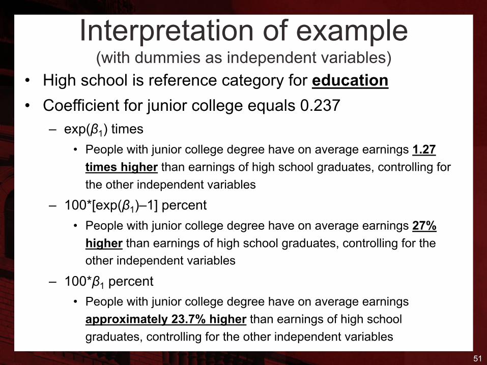
Interpretation of example(with dummies as independent variables)
• High school is reference category for education• Coefficient for junior college equals 0.237
– exp(β1) times• People with junior college degree have on average earnings 1.27
times higher than earnings of high school graduates, controlling for the other independent variables
– 100*[exp(β1)–1] percent• People with junior college degree have on average earnings 27%
higher than earnings of high school graduates, controlling for the other independent variables
– 100*β1 percent• People with junior college degree have on average earnings
approximately 23.7% higher than earnings of high school graduates, controlling for the other independent variables
51
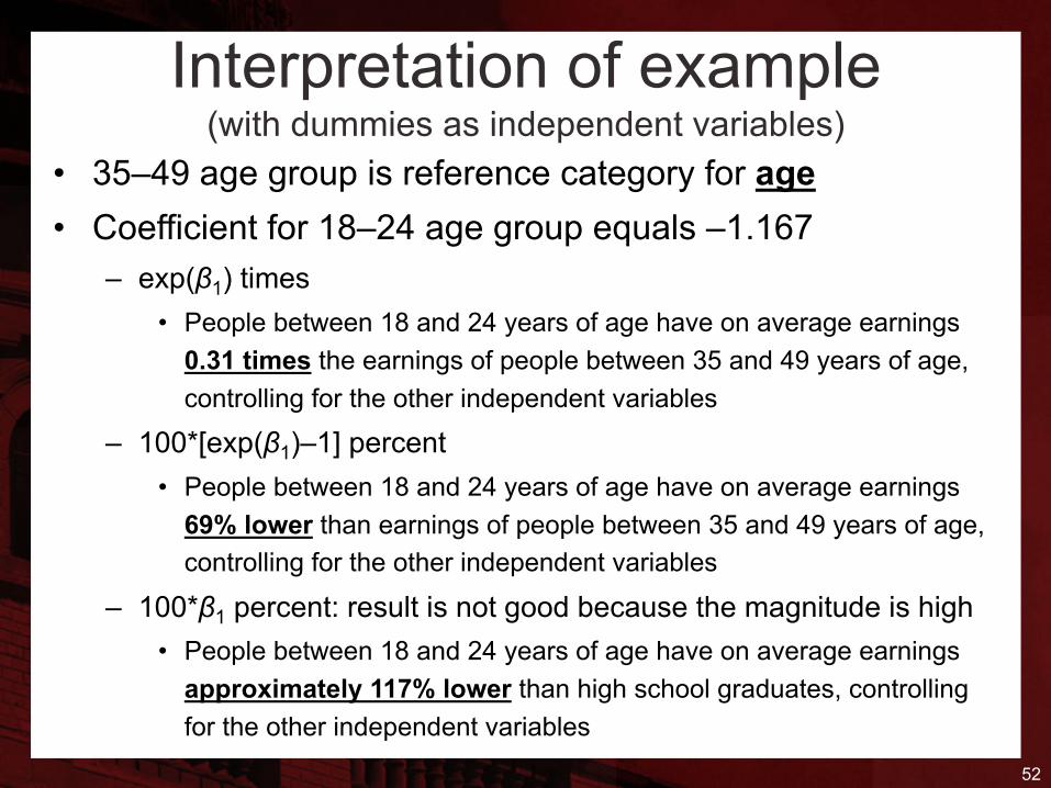
Interpretation of example(with dummies as independent variables)
• 35–49 age group is reference category for age• Coefficient for 18–24 age group equals –1.167
– exp(β1) times• People between 18 and 24 years of age have on average earnings
0.31 times the earnings of people between 35 and 49 years of age, controlling for the other independent variables
– 100*[exp(β1)–1] percent• People between 18 and 24 years of age have on average earnings
69% lower than earnings of people between 35 and 49 years of age, controlling for the other independent variables
– 100*β1 percent: result is not good because the magnitude is high• People between 18 and 24 years of age have on average earnings
approximately 117% lower than high school graduates, controlling for the other independent variables
52
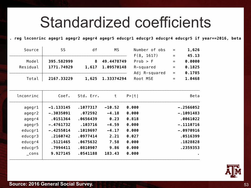
Standardized coefficients
53Source: 2016 General Social Survey.
.
_cons 9.927145 .0541188 183.43 0.000 . educgr5 .7994411 .0810907 9.86 0.000 .2359353 educgr4 .5121465 .0675632 7.58 0.000 .1828828 educgr3 .2160742 .0977414 2.21 0.027 .0516399 educgr1 -.4255014 .1019697 -4.17 0.000 -.0970916 agegr5 -.4761732 .103716 -4.59 0.000 -.1110716 agegr4 .0151364 .0656439 0.23 0.818 .0061022 agegr2 -.3035091 .072592 -4.18 0.000 -.1091483 agegr1 -1.133145 .1077317 -10.52 0.000 -.2566052 lnconrinc Coef. Std. Err. t P>|t| Beta
Total 2167.33229 1,625 1.33374294 Root MSE = 1.0468 Adj R-squared = 0.1785 Residual 1771.74929 1,617 1.09570148 R-squared = 0.1825 Model 395.582999 8 49.4478749 Prob > F = 0.0000 F(8, 1617) = 45.13 Source SS df MS Number of obs = 1,626
. reg lnconrinc agegr1 agegr2 agegr4 agegr5 educgr1 educgr3 educgr4 educgr5 if year==2016, beta
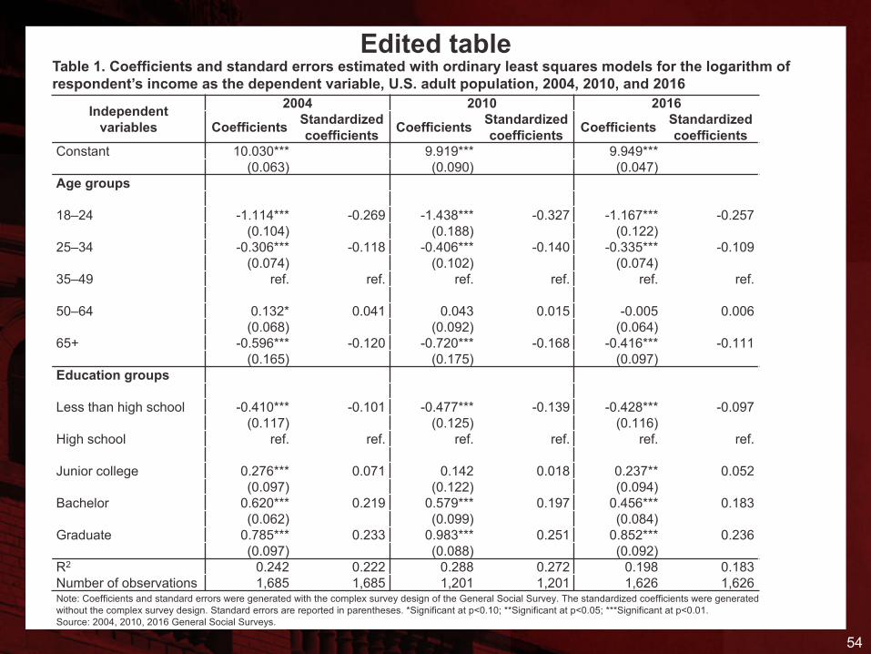
Edited table
54
Independentvariables
2004 2010 2016
Coefficients Standardizedcoefficients Coefficients Standardized
coefficients Coefficients Standardizedcoefficients
Constant 10.030*** 9.919*** 9.949***(0.063) (0.090) (0.047)
Age groups
18–24 -1.114*** -0.269 -1.438*** -0.327 -1.167*** -0.257(0.104) (0.188) (0.122)
25–34 -0.306*** -0.118 -0.406*** -0.140 -0.335*** -0.109(0.074) (0.102) (0.074)
35–49 ref. ref. ref. ref. ref. ref.
50–64 0.132* 0.041 0.043 0.015 -0.005 0.006(0.068) (0.092) (0.064)
65+ -0.596*** -0.120 -0.720*** -0.168 -0.416*** -0.111(0.165) (0.175) (0.097)
Education groups
Less than high school -0.410*** -0.101 -0.477*** -0.139 -0.428*** -0.097(0.117) (0.125) (0.116)
High school ref. ref. ref. ref. ref. ref.
Junior college 0.276*** 0.071 0.142 0.018 0.237** 0.052(0.097) (0.122) (0.094)
Bachelor 0.620*** 0.219 0.579*** 0.197 0.456*** 0.183(0.062) (0.099) (0.084)
Graduate 0.785*** 0.233 0.983*** 0.251 0.852*** 0.236(0.097) (0.088) (0.092)
R2 0.242 0.222 0.288 0.272 0.198 0.183Number of observations 1,685 1,685 1,201 1,201 1,626 1,626
Table 1. Coefficients and standard errors estimated with ordinary least squares models for the logarithm of respondent’s income as the dependent variable, U.S. adult population, 2004, 2010, and 2016
Note: Coefficients and standard errors were generated with the complex survey design of the General Social Survey. The standardized coefficients were generated without the complex survey design. Standard errors are reported in parentheses. *Significant at p<0.10; **Significant at p<0.05; ***Significant at p<0.01.Source: 2004, 2010, 2016 General Social Surveys.
Limitations• Multiple regression and correlation are among the most
powerful techniques available to researchers– But powerful techniques have high demands
• These techniques require– Every variable is measured at the interval-ratio level– Each independent variable has a linear relationship with the
dependent variable– Independent variables do not interact with each other– Independent variables are uncorrelated with each other– When these requirements are violated (as they often are), these
techniques will produce biased and/or inefficient estimates– There are more advanced techniques available to researchers
that can correct for violations of these requirements
55