1

LECTURE 28Wire Losses Due to Both Single Wire SkinEffects and Proximity Effects

A. Single Wire Losses at High Frequencies.1. Basic Copper Wire Properties2. Wire Volume, Winding Area and Current

Density, J3. Magnetic Fields and Wire Current

Distributions,J4. Cu Wire Sizes, AWG Gauge NumberSystem and Porosity of Wires5. Wire Fill Factor of a Core : Parameter K6. Core Wire Window Utilization and Porosity7. Per Unit Volume Wire Winding Losses

P(ohmic in Cu)unit volume

= J rms2ρ

8. Single Wire Conduction and Skin EffectsB. PROXIMITY EFFECTS: Enhanced Wire LossDue to Collective Effects of Contiguous Layers ofOverlapped or Interleaved Wire Windings:

1. RAC of a particular wire in a stack of wires will varywith Wire Position in a Stack

2. Proximity Effect Explained by Surface MirrorCurrents and Associated Current DensityProfiles

3. The Wire Parameter φ and Losses

2

4. Flux Strength from Non-interleavedversus Interleaved Windings

A. Increased Loss for overlapped wires via theNet MMF “M” Factor

M )(

d ~ P 2

loss fδ

d is wire diameter, δ(f) is skin depth and M isthe number of overlapped wire layers thatcontribute to the net MMF.

B. Skin Effect on J distributions in variouslayered windings and associated mmf vs x. This is the case where D>δ(skin effect).

C. Interleaving the primary and secondarywinding turns The Fractional “M” Factor

D. rms2

ACJ R losses vs the Empirical wire parameter

φ ηδ

d≡ on the x-axis of Loss Nomographs

Goal of φ ≈ 1 for low total wire loss.η depends on wire insulation’s, d is wire diameterand δ is skin effect size at the current drivefrequency.

3

LECTURE 28Wire Winding Losses due to Both Single WireSkin Effects and Proximity Effects Due to Stacksof Wire

A. Cu Wire Conduction Properties at High Frequency1. Basic Electrical Properties of Copper Wires.The electrical resistivity of the wire is given by the parameterρ= 2.2 * 10-6 Ω -m @100oC and ρ= 1.7 * 10-6 Ω -m @20oC. We tryhard not to have the wire temperature exceed 100oC becausecores, wires and solid state devices all degrade at highertemperatures

High σ or equivalently low ρ means that in a wire of length land cross-sectional area A the total DC wire resistance is

)A()l( = )R(

wirewireDC ρ .

Next we calculate the DC resistance of a length of wire. Let’sconsider a simple case of a primary wire winding used in atransformer, wound around a magnetic core cross-section ofperimeter 10 cm. The core has an open wire-winding window intowhich the wire is placed. The total winding would usually entail anumber of turns to achieve the desired value of the magnetizinginductance for the transformer

For a primary winding of n turns around a 10 cm perimetercore we might estimate the total length of wire for n turns as :

L = n*10 meters. Hence the DC resistance of the wire is:Rprimary = RL(AWG Wire #) in Ω /m * L

For example, for #19 wire RL = 27 mΩ /m at 25°C. So for 60 meters of wire

Rprimary = 1.6 ΩThis wire resistance value will hold only for DC currents and is notaccurate as the frequency of the current is increased. We findherein that this simple-minded DC result is as much as a factor

4

of 10-1000 too low in resistance from those measured at highfrequency. This is due to several effects that occur due tointeractions between an external magnetic field and current flow ina wire that this magnetic field passes through.

2. Wire Volume, Winding Area and Current Density,JWe always seek to use the minimum area wire required for

cost reasons when winding any inductor or transformer on amagnetic core. That is with larger diameter wire, and a fixednumber of turns required, the core size must be increased to fit thewire coil. Also with smaller diameter wire we employ a smalleramount of associated wire volume on any inductor or atransformer. However, minimum size wire means the currentdensity in the wire will increase, J ↑, for a given wire current andhence the power loss per unit volume will go as P ~ ρJ2.

The primary and secondary wire sizes in a transformer will beset such that J is the same in the primary and secondary wires. Otherwise the heat loss per unit volume will be mismatched in thetwo windings and optimum heat generation will not occur. In shortone winding will overheat before another and be damaged. Wewill show later tradeoffs between Cu wire volume and magneticmaterial volume to minimize total undesired heating from bothwires and magnetic cores.

The wire material of choice is copper. The high ductility ofCu makes tight windings with sharp bends easy to achieve onsmall size magnetic cores. Tight windings also mean a minimumvolume of Cu employed. Never forget that the permeability ofcopper is the same as that of air so any magnetic field will passthrough the wires as easily as through air. Second, due to therelatively small (100-10,000 times µ0) permeability’s of magneticmaterials substantial leakage flux occurs outside the core. Thismeans that leakage flux from magnetic cores will easily leavethe core and enter the wires wound around the cores. Thisleakage flux in the wires causes high currents to flow at the wiresurfaces, which in turn will change the effective wire resistance,

5

especially to high frequency currents as we shall see in parts Band C below.

3. Magnetic Fields and Wire Current Distributions, JWe will divide these magnetic field- wire interaction

phenomena into two parts.One is for isolated wires carrying current and is termed the

skin effect. Skin-effects in a single isolated wire are due to themagnetic field from the current flow itself penetrating the wire andcausing internal eddy currents in the conductive wire. We alreadycovered skin effects in Lecture 26.

The second effect is the interaction between collectivemagnetic fields created by turns of wires on the current flowing inindividual wires and is termed the proximity effects in stackedlayers of wires. A quick insight into collective magnetic effectsfrom different choices of winding wire coils is as follows. Considerthe difference in H fields we achieve when we wind a coil of nturns in a single layer on a large core of magnetic length x. Compare this result versus the result if we wind the same n turnsin several stacks on a smaller size core of magnetic length x/10. The latter small size core will require one to employ multiplestacked layers of wires on top of each other to fit N turns, if thecore wire winding window did not have sufficient height to fit allrequired wire turns in one layer. This opens up the subtle detailsof wire winding configurations on the cores.

We will see that one long layer of wire turns, on a core oflength x, has less magnetic field generated than a stack of wireson a core of length x/10. This occurs due to Ampere’s law whichsays Ni=H x. H differs if all N turns fit along the length x ascompared to if the N turns are in multiple layers along a smallercore length x/10. We will revisit this in sections B and C belowwhere the H field that enters the wires will cause large mirrorcurrents to flow that increase wire loss above that from skin effectsalone.

6

5. Cu Wire Sizes, AWG Gauge Number System andPorosity of Wires

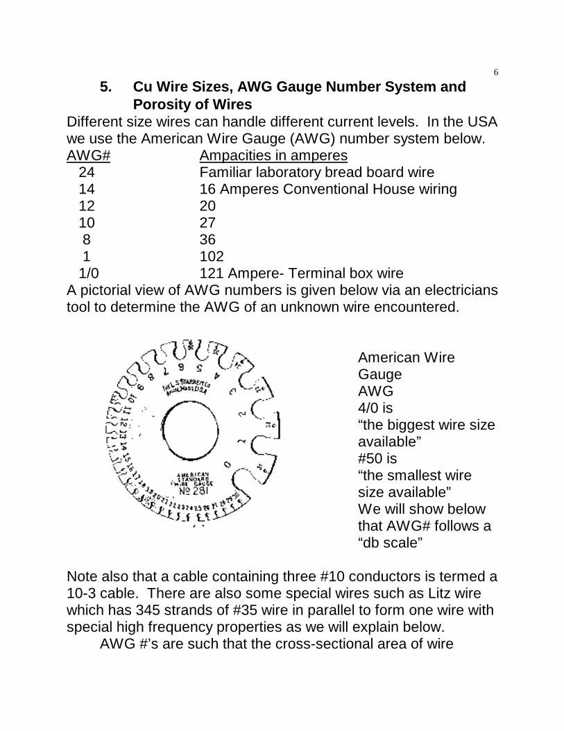
Different size wires can handle different current levels. In the USAwe use the American Wire Gauge (AWG) number system below.AWG# Ampacities in amperes 24 Familiar laboratory bread board wire 14 16 Amperes Conventional House wiring 12 20 10 27 8 36 1 102 1/0 121 Ampere- Terminal box wireA pictorial view of AWG numbers is given below via an electricianstool to determine the AWG of an unknown wire encountered.

American WireGaugeAWG4/0 is“the biggest wire sizeavailable”#50 is“the smallest wiresize available”We will show belowthat AWG# follows a“db scale”

Note also that a cable containing three #10 conductors is termed a10-3 cable. There are also some special wires such as Litz wirewhich has 345 strands of #35 wire in parallel to form one wire withspecial high frequency properties as we will explain below.

AWG #’s are such that the cross-sectional area of wire

7

doubles every change of 3 AWG sizes. That is in term of wirediameters , AWG wire changes are like base 10 decibels in that ifone increases or decrease AWG # by 20, the wire diameterdecreases or increases by a factor of ten respectively. Thus forexample, #10 wire has ten times the diameter of #30 wire.

Some other factoids about the AWG systemIncrease AWG # by 6 and we find the diameter varies by D/2Increase AWG # by 10 and we find the wire cross-section areavaries as Area/10Increase AWG # by 3 and the wire area changes by Aw/2

Wire area seems a simple concept but there is a very troublesomeunit of wire area for metric challenged U.S. engineers that causeslots of headaches. This is the concept of circular mils.

mil Area of square 1 mil on a side is (mil)2

In the USA we define a Circle inside the square as 1circular mil. This unfortunately is the standard. Thusa1 cm2 area is then 200,000 cir mils in USA units

Next we consider conductor spacing factor or porosity for differentshape wires. For example to achieve the wire turns required, wecould use round shape wire, square shape wire and even tape likewire. Clearly, each shape wire would have a different porosity ordensity of turns. We use a symbol η for this wire porosityparameter from which we get an effective wire diameter:deff =d(actual wire diameter) η . Again η is termed the wire porosityand is specified by the wire manufacturer for each type of wiregeometry. Roughly speaking, voids between wires waste 21% ofthe winding cross-section area. Wire insulation further reducesthe useful area, especially with the smaller diameter wires used tominimize high frequency losses, because insulation is a largerpercentage of small wire diameters.

5. Magnetic Core Cu Wire Fill FactorThe wire size and required number of turns to a great extenddictate the magnetic core size needed for either an inductor or a

8

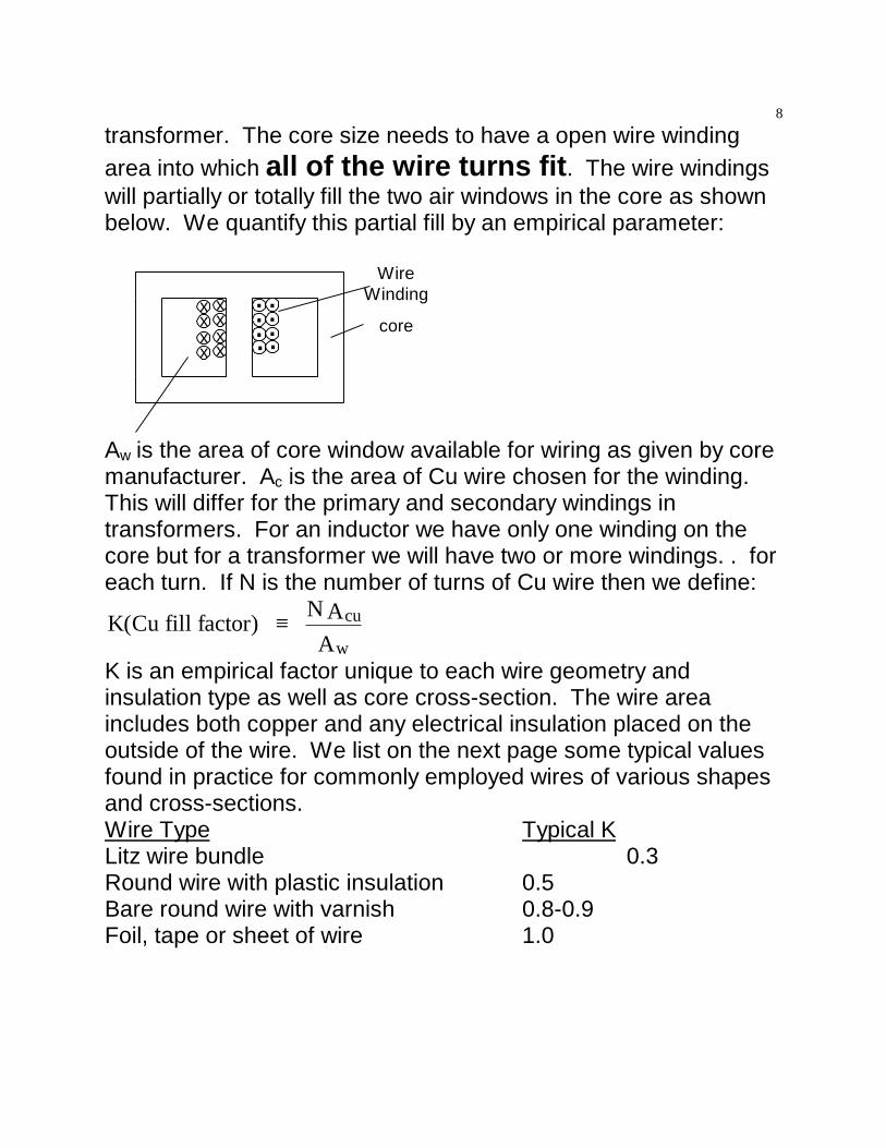
transformer. The core size needs to have a open wire windingarea into which all of the wire turns fit. The wire windingswill partially or totally fill the two air windows in the core as shownbelow. We quantify this partial fill by an empirical parameter:

........x

xxx

xxxx

WireWinding

core

Aw is the area of core window available for wiring as given by coremanufacturer. Ac is the area of Cu wire chosen for the winding. This will differ for the primary and secondary windings intransformers. For an inductor we have only one winding on thecore but for a transformer we will have two or more windings. . foreach turn. If N is the number of turns of Cu wire then we define:

K(Cu fill factor) N AA

cu

w≡

K is an empirical factor unique to each wire geometry andinsulation type as well as core cross-section. The wire areaincludes both copper and any electrical insulation placed on theoutside of the wire. We list on the next page some typical valuesfound in practice for commonly employed wires of various shapesand cross-sections.Wire Type Typical KLitz wire bundle 0.3Round wire with plastic insulation 0.5Bare round wire with varnish 0.8-0.9 Foil, tape or sheet of wire 1.0

9

6. Core Wire Window Utilization and Wire PorosityWe ask -How large a core window is necessary to contain

the ampere-turns of all the required windings on a transformer?. Ultimately, this is determined by maximum allowable powerdissipation in both the core and in the wire windings. This powermust be dissipated as heat flow from the core/wire winding massto the ambient. The balance between heat generated and heatflow from the core/winding mass to the environment causes anequilibrium associated temperature rise. In practice this must nowexceed 100 degrees C where wire insulation degrades as do thecore magnetic properties.

Assuming we do not violate equilibrium temperatures foreither the wire or the core we now ask the question in a simplerway. How much of the window area is actually useful copper areawhere current flows? A wire winding bobbin, if used, significantlyreduces the available window area, again impacting smaller, lowpower applications. In a small transformer with a bobbin and withhigh voltage isolation requirements, perhaps only 25% or 30% ofthe window area is actually current carrying copper. Electricalcodes impose voltage isolation safety requirements ontransformers such as the need for 3 layers of insulation betweenprimary and secondary windings. We also must insure minimumleakage or creepage distances of 6 to 8mm from primary windingsto secondary windings where leakage current may flow around theends of the insulation layers at both ends of the winding. Nearly 1cm of window breadth is lost to this safety requirement, severelyimpacting window utilization, especially with smaller cores in lowpower transformers. The increased separation between primaryand secondary coils also results in higher leakage inductance inthe transformer, as we will see later.

Below we consider the window winding area of a givenmagnetic core is h high by IW wide in area. We revisit theempirical parameter called the wire porosity.

10

lw Consider that in a stack of turns h high by lw wide weplace a n turns employing wire of diameter d. We cansay that the wire porosity is:

η π

wiring

porosity d

nlw

≡ ≡4

2

h.7 < η < .8 is typical for a range of insulated wires.Note that η reduces the effective conductivity of the wire, orincreases the effective resistivity of a wire, because the wireinsulation takes up area that is not employed for current flow.In short η becomes the Effective diameter of wire:

effd = d η - Typically η introduces a factor of 0.9

eff 2 effR = l( )A

= l( )d4

But d = d( )ρ ρ

πη ρ

π η

wire wire l wiredw eff

⇒ 2

4

= R/η

Higher R in the wire means Higher I2R losses for fixed currentflow! The load not the wires determines current flow.

In summary, eff geometryR ~ 1

* Rη(without porosity corrections)

7. Power Dissipated Per Volume in the Wire WindingsWe will consider equilibrium heat flow in lecture 29 including wireand core losses together. Because heat equations and corelosses use input heat in P/cm3 we need to find wire losses in thesame units of W/cm3.

powerP(per unit volume) = cuρ (Ω -cm ) rms

2J (A/ cm )2 2 in W/cm3 units of copperA traditional rule-of-thumb for mains 50-6OHz transformers is tooperate copper windings at a current density of 450 A/cm2(2900A/in2). However, smaller high frequency transformers can operateat higher current densities because there is much more heat

11

dissipating surface area in proportion to the heat generatingvolume.The effective wire volume used for heat flow is actually smaller bythe factor K as we saw above. That is the winding volume is:

V * )factor

fillk( = V wcu

Cu (core window volume)

For ρ= 2.2 * 10-8 Ω -m and J in A/mm2 units which is more usefulthan A/cm2 we find:

J )K( 22 = ) volumewinding

perpower P( 2

rmsfillfactor units mW/cm3

8. Single Wire Conduction and Skin Effects

a. H fields Surrounding WiresOne wire with DC current flowing causes a magnetic field that isboth enclosing and penetrating the wire. The H field intensityoutside the wire versus current flow within is given by by AmperesLaw: ∫H•dl = H2πr = I. That is H(outside the wire) =I/2πR. Thefield decays with the distance form the outer radius of the wire. Inside the wire, for a constant DC current distribution versus wireradius, H can be shown to increase linearly with radius, starting atzero at r=o and increasing to HMAX at the wire radius, r=a.

B

A

AB

H1/L

12

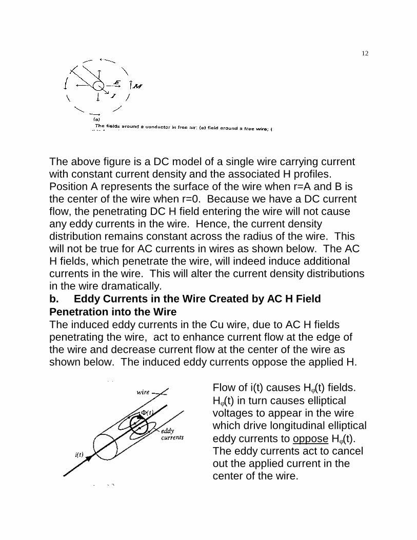
The above figure is a DC model of a single wire carrying currentwith constant current density and the associated H profiles. Position A represents the surface of the wire when r=A and B isthe center of the wire when r=0. Because we have a DC currentflow, the penetrating DC H field entering the wire will not causeany eddy currents in the wire. Hence, the current densitydistribution remains constant across the radius of the wire. Thiswill not be true for AC currents in wires as shown below. The ACH fields, which penetrate the wire, will indeed induce additionalcurrents in the wire. This will alter the current density distributionsin the wire dramatically.b. Eddy Currents in the Wire Created by AC H FieldPenetration into the WireThe induced eddy currents in the Cu wire, due to AC H fieldspenetrating the wire, act to enhance current flow at the edge ofthe wire and decrease current flow at the center of the wire asshown below. The induced eddy currents oppose the applied H.

Flow of i(t) causes Hφ(t) fields.Hφ(t) in turn causes ellipticalvoltages to appear in the wirewhich drive longitudinal ellipticaleddy currents to oppose Hφ(t). The eddy currents act to cancelout the applied current in thecenter of the wire.

13

Looking at a wire cross-section above better explains the neteffect on the J(r) profile to reduce current flow in the middle of thewire.

Current flows in the wire path(s) that result in the lowestexpenditure of energy. At low frequency, this is accomplished byminimizing I2R losses and constant current density profiles of DCcurrents result. At high frequency, current flow in the path(s) thatminimizes inductive energy dominates. That is, energy transfer toand from the magnetic field generated by the current flow. Energyconservation causes high frequency current to flow near thesurface of a thick conductor even though this may result in muchhigher I2R losses. If there are several available paths, HF currentwill take the path(s) that minimize inductive energy.

FOR HW# 6 derive and plot the same currentdensity and H versus radius profiles for highfrequency currents. Be as quantitative aspossible. Employ the handout of Bessel function currentprofiles from Professor Collins to derive current density and Hprofiles versus radius as shown below.J decays exponentially from the outer surface of the wire towardsthe center with a spatial decay constant δ, J(r) ~ e-r/δ as shown.

d

J(r) in wire

exp-r/δ δ ρπµ

f

≡

Using constants for Cu media we find:

δ(cu @100oC) = 7.5 cm

f

14

Frequency 50 Hz +|5 KHz |20 KHz |500 KHzδ(skin depth) 10.6 mm |1.06 mm |1/2 mm |0.106 mm

B. PROXIMITY EFFECTS: Collective Effects ofLayers of wiring

1. RAC of a Particular Wire in a Stack of Wires will vary withWire Position in a StackFor single conductors of size d(wire diameter) > δ(Skin depth) weexpect simple resistance changes at high frequency as compared

to DC. Consider for a single wire various values of dδ

for #20

AWG wire and the effects of RAC for a single wire as shown below.

ac dcR = R (d

)δ

d = 1000µ

f | d/δ(µ) RAc/RDC Ratio 104 | 300 | 3.3 106 | 80 | 12.5

Surprisingly for two wires next to each other Rac/Rdc exceedsthis single wire skin effect value due to proximity effects of severalwires causing a collective magnetic field. That is when we wrapseveral layers of wire turns next to each other we find that Rac >Rdc by more than expected from simple single wire skin effects asdiscussed in part A due to collective H fields being created by thewire stack. Depending on the location of the wire we penetratedifferent wires with different H levels. The net currents in anysingle wire do not change but the current consists of mirrorcurrents of opposite direction flowing on the outer surfaces. These are called proximity effects, which further increase Racabove the values for single isolated wires, as we will show below. That is Reff increases above simple skin effect values due to thecumulative proximity effect of N turns of wire. Recall, NI = H x

15

(magnetic path length). Moreover, the resistivity increase due toproximity effects in any one wire now depends on the wire positionin the cumulative magnetic field pattern. Different cumulative Harises after each wiring layer is added for fixed current, I, andmagnetic path length,x, as described below.

Looking ahead, the additional resistance for a second layerof wiring in a multi-turn wiring stack will be 5 times that of the firstlayer of wiring. This occurs because 2xI flows on one wire surfaceand I flows on an opposing surface in the opposite direction. Thenet current in the wire is unchanged at I. But the I2R losses arefive times as great. The resistance of the third layer will be 13times as large expected as shown below on page 21 due to 3xIflowing on one surface and 2xI flowing on the opposite surface.

We next set down the basic details of the proximity effect toexplain better why we have surface current flowsin opposite directions on the same wire prior toquantifying resistivity increases.

2. Proximity Effect Explained by Surface MirrorCurrents and Associated Current DensityProfiles

a. Overview of Conditions that Alter Current ProfilesWhen two conductors are in near proximity and carry

opposing high frequency currents, the current density distributionsin each wire spread across the entire opposing wire surfacesfacing each other in order to minimize the total magnetic fieldenergy transfer (minimizing inductance). That is current flow in thewire cross-section, l x w shown below, fills the entire length l of thewire shown below BUT DOES NOT fill the entire width w of thewire. These non-uniform spatial current density profiles will causeunique I2R losses. Recall that NI=Hl. As l increases H willdecrease. The above fully spatially extended , high frequency

16

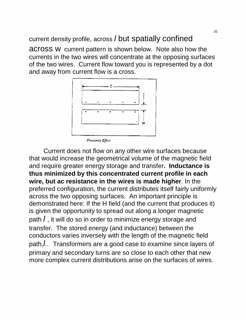
current density profile, across l but spatially confinedacross w current pattern is shown below. Note also how thecurrents in the two wires will concentrate at the opposing surfacesof the two wires. Current flow toward you is represented by a dotand away from current flow is a cross.

Current does not flow on any other wire surfaces becausethat would increase the geometrical volume of the magnetic fieldand require greater energy storage and transfer. Inductance isthus minimized by this concentrated current profile in eachwire, but ac resistance in the wires is made higher. In thepreferred configuration, the current distributes itself fairly uniformlyacross the two opposing surfaces. An important principle isdemonstrated here: If the H field (and the current that produces it)is given the opportunity to spread out along a longer magneticpath l , it will do so in order to minimize energy storage andtransfer. The stored energy (and inductance) between theconductors varies inversely with the length of the magnetic fieldpath,l.. Transformers are a good case to examine since layers ofprimary and secondary turns are so close to each other that newmore complex current distributions arise on the surfaces of wires.

17

b. One Layer of Turns and Wire Current Distributions in aTransformerA given transformer shown below has two windings, which fit

in one layer of turns. Two cases will be explored. Each dot orcross in the wires represents one Ampere of current flow. Theprimary carries 3A and the secondary 12A in the one case wherethe four turn primary wires are connected in series. This couldbe the case for a 4-turn primary winding carrying 3A, opposed by asingle turn secondary carrying 12A.

In a second transformer winding case, the four primary wirescould be connected in parallel, giving a effective 1-turn primarycarrying 12A with 12 A flowing in a single turn secondary.

When the conductors are thicker than the skin effect size,δ, thehigh frequency currents flow near the surfaces of the wires inclosest proximity, thus terminating the magnetic field withminimum energy. In either case, the H field pattern spreadsitself across the entire wire-winding window and theminimized energy is stored between the windings if thecurrent flow is altered as shown below. The currents aredriven to the surfaces of the wires by the minimization of magneticenergy.

The above case is for single stacks of primary and secondary wirewindings. The case of multiple stacks of wire winding is next.

18

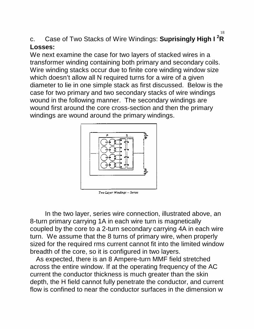
c. Case of Two Stacks of Wire Windings: Suprisingly High I 2RLosses:We next examine the case for two layers of stacked wires in atransformer winding containing both primary and secondary coils. Wire winding stacks occur due to finite core winding window sizewhich doesn’t allow all N required turns for a wire of a givendiameter to lie in one simple stack as first discussed. Below is thecase for two primary and two secondary stacks of wire windingswound in the following manner. The secondary windings arewound first around the core cross-section and then the primarywindings are wound around the primary windings.

In the two layer, series wire connection, illustrated above, an8-turn primary carrying 1A in each wire turn is magneticallycoupled by the core to a 2-turn secondary carrying 4A in each wireturn. We assume that the 8 turns of primary wire, when properlysized for the required rms current cannot fit into the limited windowbreadth of the core, so it is configured in two layers.

As expected, there is an 8 Ampere-turn MMF field stretchedacross the entire window. If at the operating frequency of the ACcurrent the conductor thickness is much greater than the skindepth, the H field cannot fully penetrate the conductor, and currentflow is confined to near the conductor surfaces in the dimension w

19

but extends fully in the dimension l. This is illustrated by the dot

and cross current flows in the wires. Note that the innersecondary winding and the outer primary windinghave surface currents just like our first case of singlelayer windings discussed above.

A strange thing happens, however, to current profiles inthe w direction at the interface between the primary andsecondary wire windings only. Here the first primary wirecarries a net 1A but 2A in the cross-direction are on one wiresurface facing the primary and 1A in the dot direction flows on thesurface of the outer primary wire. The interface termination ofcurrents via associated H fields is associated with mirror currentsin the opposite sides of the respective wires of magnitudes asdescribed below. The two wires involved with mirror currents areonly the first turn of the primary winding and the second term ofthe secondary. The second term of the primary and the first ternof the secondary have no mirror currents on opposite surfaces justas the single layer case.

We first deal with the surface currents at the inner surface ofthe first turn of the primary and the outer surface of thesecond turn of the secondary. Since the H field cannot fullypenetrate the wire conductor, an 8A driven H field terminates atthe inner surface of the first primary turn and at the outer surfaceof the second turn of the secondary wires as shown above. Adding the dots and crosses in the outer turn of the secondary weend up with a net current of 4 A in this turn as seen from outsidethe wire. Likewise the total current from outside the wire in thefirst primary winding is 4A in the cross-direction, with 8A in thecross-direction at the inner surface and 4A at the outer surface inthe dot direction for a net 4A. The two current density segmentsare flowing on opposite surfaces of the same wire. This occursonly for the turns layer of the primary that face the secondarywinding and vice versa. The far left primary winding and the far

20

right secondary winding carry current only in the cross directionand the dot direction respectively..

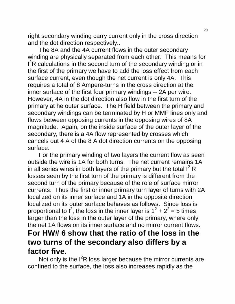
The 8A and the 4A current flows in the outer secondarywinding are physically separated from each other. This means forI2R calculations in the second turn of the secondary winding or inthe first of the primary we have to add the loss effect from eachsurface current, even though the net current is only 4A. Thisrequires a total of 8 Ampere-turns in the cross direction at theinner surface of the first four primary windings -- 2A per wire. However, 4A in the dot direction also flow in the first turn of theprimary at he outer surface. The H field between the primary andsecondary windings can be terminated by H or MMF lines only andflows between opposing currents in the opposing wires of 8Amagnitude. Again, on the inside surface of the outer layer of thesecondary, there is a 4A flow represented by crosses whichcancels out 4 A of the 8 A dot direction currents on the opposingsurface.

For the primary winding of two layers the current flow as seenoutside the wire is 1A for both turns. The net current remains 1Ain all series wires in both layers of the primary but the total I2 Rlosses seen by the first turn of the primary is different from thesecond turn of the primary because of the role of surface mirrorcurrents. Thus the first or inner primary turn layer of turns with 2Alocalized on its inner surface and 1A in the opposite directionlocalized on its outer surface behaves as follows. Since loss isproportional to I2, the loss in the inner layer is 12 + 22 = 5 timeslarger than the loss in the outer layer of the primary, where onlythe net 1A flows on its inner surface and no mirror current flows. For HW# 6 show that the ratio of the loss in thetwo turns of the secondary also differs by afactor five.

Not only is the I2R loss larger because the mirror currents areconfined to the surface, the loss also increases rapidly as the

21

number of layers of turns employed increases as we show below. This is because the field intensity increases progressively towardthe inside of the winding and PEAKS at the primary to secondaryinterface. Since the field cannot penetrate the conductors, surfacecurrents must also increase progressively in the inner layers. Forexample, if there were 6 wire layers, all wires in series carrying 1A,then each wire in the inner layer will have 6A flowing on its innersurface (facing the secondary winding) and 5A in the oppositedirection on its outer surface. The loss in the inner layer is 62 + 52

= 61 times large than in the outer layer which has only the net 1Aflowing on its inner surface!

All of the above surface mirror current flow was predicated onthe wire diameter being much greater than the skin depth at theoperating frequency of the current in the wire. If the wirediameter is reduced to that approaching the skin depth, the +and - currents on the inner and outer surfaces of each wirestart to merge, partially canceling and thereby reducing I2Rlosses in the wires located at the interface of primary andsecondary. The H field now partially penetrates through theconductor. When the wire diameter is much less than thepenetration depth, the field penetrates completely, the opposingcurrents at the surfaces completely merge and cancel, and the 1Acurrent flow in the primary is distributed throughout each wire ofthe primary uniformly.

Calculation of the I2R loss in the multi-layer turn coil where thewire diameter well exceeds the skin depth is very complexdepending primarily on the number of layers in each windingsection. In summary, we find for multi-layered windings the powerloss,PM, for each layer,m, goes as shown on page 22.

22

Pm = P1 [(m-1)2+ m2]

P3 = I32(rms) Rac (22+32)= 13P1

P2 = I22(rms) Rac (22+12)= 5 P1

P1 = 1rms2

acI R

We repeat, in stark contrast, for wire diameters and operating wirecurrent frequencies such that d ~ δ, in a coil of M layers each layercarrying the same total current Ptotal = MP1One can show that for wires and operating frequencies such that d>> δ the total loss of all layers together is:

totalj=1

Mj

21P = P =

M3

(2 M + 1) P∑ Only for d >> δ

The most difficult case to model is for depthskind .~ in each wire withM layers of windings the I 2R loss has two factors when normalizedto the DC loss case which we state but do not derive:

AC

DCR

2PP

= F = d

2 M +1

3δ

↓ ↓The single wire factor d/δ varies from 2-8. The second factor isnot negligible and can easily be a factor of *10 even *100

Consider the term | M | 2 m + 1

3

2

23

Depending on M we get for example. M=1 we get a factor of 1 butfor M=3 we could get a factor of 6, while for M=10 a factor of 60may occur.

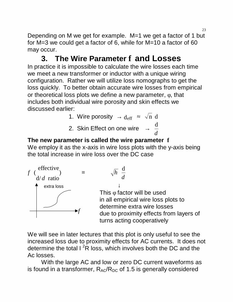
3. The Wire Parameter φ and LossesIn practice it is impossible to calculate the wire losses each timewe meet a new transformer or inductor with a unique wiringconfiguration. Rather we will utilize loss nomographs to get theloss quickly. To better obtain accurate wire losses from empiricalor theoretical loss plots we define a new parameter, φ, thatincludes both individual wire porosity and skin effects wediscussed earlier:

1. Wire porosity → ≈effd n d

2. Skin Effect on one wire → dδ

The new parameter is called the wire parameter φ We employ it as the x-axis in wire loss plots with the y-axis beingthe total increase in wire loss over the DC case

φδ

ηδ

(effective

d/ ratio)

d≡

φ

extra loss ↓ This φ factor will be used in all empirical wire loss plots to determine extra wire losses due to proximity effects from layers of turns acting cooperatively

We will see in later lectures that this plot is only useful to see theincreased loss due to proximity effects for AC currents. It does notdetermine the total I 2R loss, which involves both the DC and theAc losses.

With the large AC and low or zero DC current waveforms asis found in a transformer, RAC/RDC of 1.5 is generally considered

24

the optimum wire loss goal. Of course poorly designedtransformers can have loss factors of 10 –100 as seen from anyloss nomograph plot whose vertical axis extends to 100 times DCloss.

Achieving a lower RAC/RDC ratio requires finer wire to beemployed in the windings, and the wire insulation and voidsbetween wires further reduces the amount of copper. The endresult is while we decrease AC losses we end up with in higher dclosses. In a typical filter inductor with small ac ripple currentcomponent, a much larger RAC/RDC can be tolerated and we do notwant to increase DC losses as the DC component of current oftenexceeds the AC component.

4. Variation of Flux Strength from StackedWindings: Non-interleaved versus InterleavedWindingsWindings need not be wired with the primary and then thesecondary windings. We can interleave the windings with aportion of the primary followed by a portion of the secondary. Thisinterleaving brings big benefits to the total losses as we will seebelow.Consider a transformer-wiring stack placed along the x direction ofthe core-winding window. We have m (primary) coils wound firstwith current flow in one direction next to a series stack ofn(secondary coils) with current in the opposite direction. Bothstacks encircle a common magnetic core. If we plot mmf versusdistance in the wire-winding window, x, from the interleavedwindings we get very unique MMF plots as compared to the casewithout interleaving. We first look at non-interleaved for the twocases below for wire size larger (part 4b) and less than(part 4a)skin depth and vice versa. Then we address the case ofinterleaved windings in 4c. Finally in section 4d we calculate thelosses for the interleaved case.

25

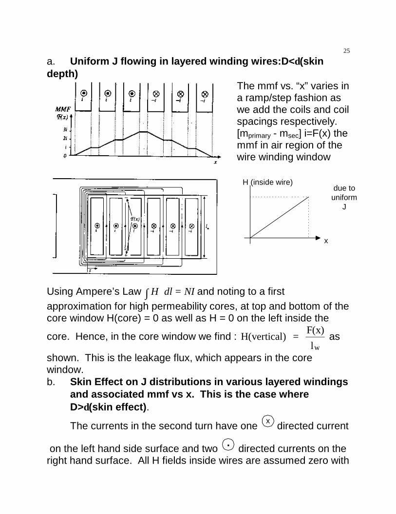
a. Uniform J flowing in layered winding wires:D<δ(skindepth)

The mmf vs. “x” varies ina ramp/step fashion aswe add the coils and coilspacings respectively.[mprimary - msec] i=F(x) themmf in air region of thewire winding window

x

H (inside wire)due to

uniformJ

Using Ampere’s Law H dl NI⋅ =∫ and noting to a firstapproximation for high permeability cores, at top and bottom of thecore window H(core) = 0 as well as H = 0 on the left inside the

core. Hence, in the core window we find : H(vertical) = F(x)lw

as

shown. This is the leakage flux, which appears in the corewindow.b. Skin Effect on J distributions in various layered windings

and associated mmf vs x. This is the case whereD>δ(skin effect).

The currents in the second turn have one x directed current

on the left hand side surface and two . directed currents on theright hand surface. All H fields inside wires are assumed zero with

26

the J distributed only at the edge of the wire due to Ampere’s law. This causes F(x) to vary in a trapezoidal bar graph fashion ratherthan in ramp/step fashion when J was uniform inside the wire.

xd

J

∫ • ≡ ∫ • H dl J dAr r

= IH exists only atthe outside ofthe wire where ?J? dA is non-zero

Peak F(x) at 3*I just at the primary-secondary interface

c. Interleaving the primary and secondary winding turnsacts to reshape mmf vs x patterns in the core wire winding windowas shown below. Two interleaving wiring patterns are shownbelow. Note that fractional NET M values of ½ or 3/2 etc are nowpossible, whereas in the non-interleaved windings only integervalues were possible.

For alternating primary/secondary For a 2-3-2 alternatingwindingwindings. pattern.

Fmax = i Fmax = 1.5 iNote we can both set (mmf)max and tailor its spatial profile bychoice of interleave patterns of the wire windings.

27

Spatial location of the zeros of F(x) may also be tailored as toprecise x spatial location they occur by tailoring net (mp-ms) = 0locations as shown above.

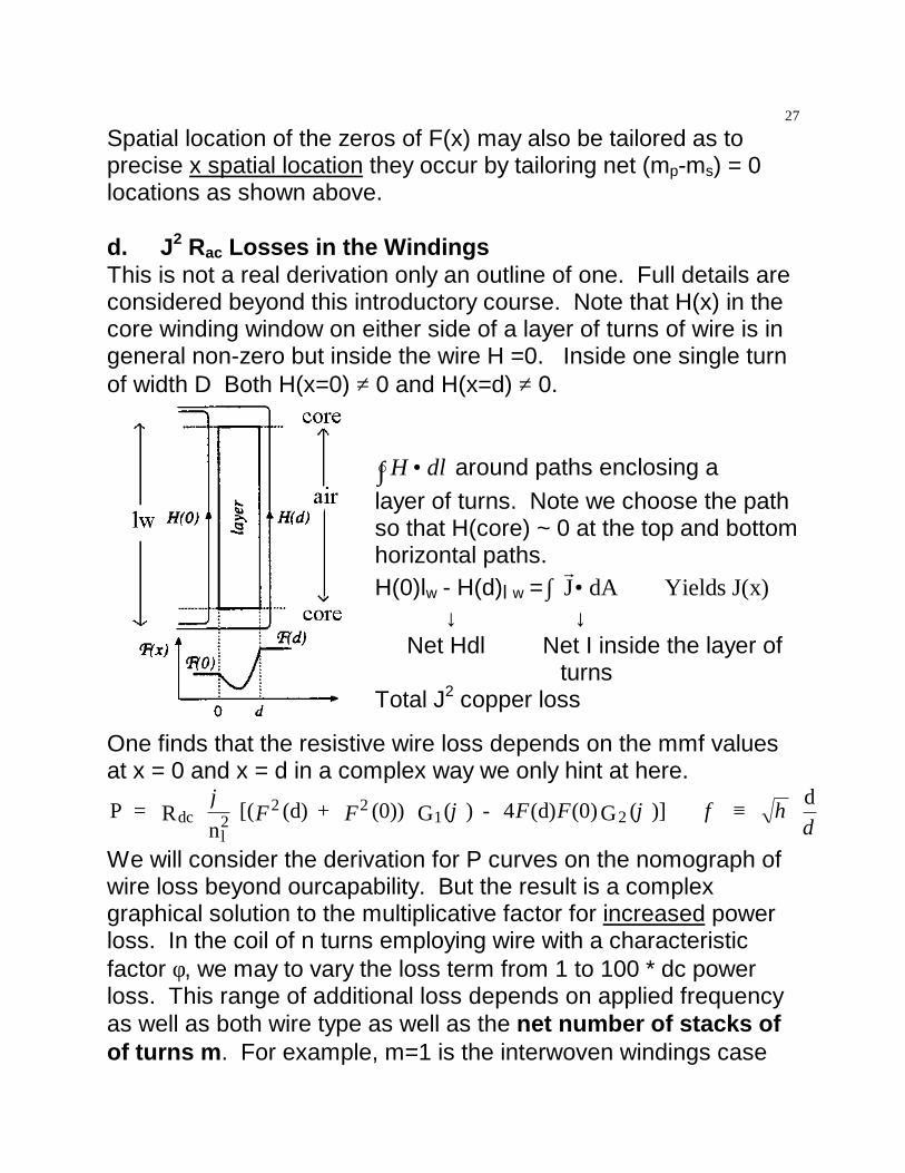
d. J2 Rac Losses in the WindingsThis is not a real derivation only an outline of one. Full details areconsidered beyond this introductory course. Note that H(x) in thecore winding window on either side of a layer of turns of wire is ingeneral non-zero but inside the wire H =0. Inside one single turnof width D Both H(x=0) ≠ 0 and H(x=d) ≠ 0.

H dl•∫ around paths enclosing alayer of turns. Note we choose the pathso that H(core) ~ 0 at the top and bottomhorizontal paths.H(0)lw - H(d)l w =∫ • ⇒ J dA Yields J(x)

r

↓ ↓ Net Hdl Net I inside the layer of turnsTotal J2 copper loss

One finds that the resistive wire loss depends on the mmf valuesat x = 0 and x = d in a complex way we only hint at here.

P = R n

[( (d) + (0)) G ( ) - 4 (d) (0) G ( )] d

dcl2

2 21 2

ϕ ϕ ϕ φ ηδF F F F ≡

We will consider the derivation for P curves on the nomograph ofwire loss beyond ourcapability. But the result is a complexgraphical solution to the multiplicative factor for increased powerloss. In the coil of n turns employing wire with a characteristicfactor φ, we may to vary the loss term from 1 to 100 * dc powerloss. This range of additional loss depends on applied frequencyas well as both wire type as well as the net number of stacks ofof turns m. For example, m=1 is the interwoven windings case

28

with one turn of primary followed by one turn of secondary. Thiscauses the square-wave like mmf pattern versus distance shownon page 26. In general, in wire loss plots m is the ratio of themmf, F(d), to the layers ampere turns nli. and is the scalingparameter as shown below. The factor φ is used for the x-axis and

the Ac loss to DC loss ratio is the y-axis. Note again φ ηδ

= d

At ϕ = 10 in the winding loss plot there is strong proximity effectobserved since d/δ= 10 and skin effects will cause a big increasein R depending on the NET # of layers of turns m as shown below.P/(I2Rdc) = (Actual Loss) / (expected dc loss)Clearly m=1 or the interleaved primary and secondary windings isa desired low loss case as compared to m=10. For low loss wirewindings we need to heed the interleaving versus non-interleaved.

In calculating theincreased loss we ask.1. Where does Litz wire

lie?2. Where do lossesfrom harmonicfrequencies as forexample from a squarewave excitation lie?The normalizing factor isPdc for d = δ.

For HW# 6 explain the physical situation for thewire windings that creates m=1/2There is no benefit in pushing to an RAC/RDC of 1.5 by arbitrarlymaking the φ factor on the x-axis smaller. If via the φ factorreduction for minimizing RAC the RDC is increased to two or threetimes we have not really saved anything except in transformerswhere I DC is zero. In an inductor where the DC and AC signals

29

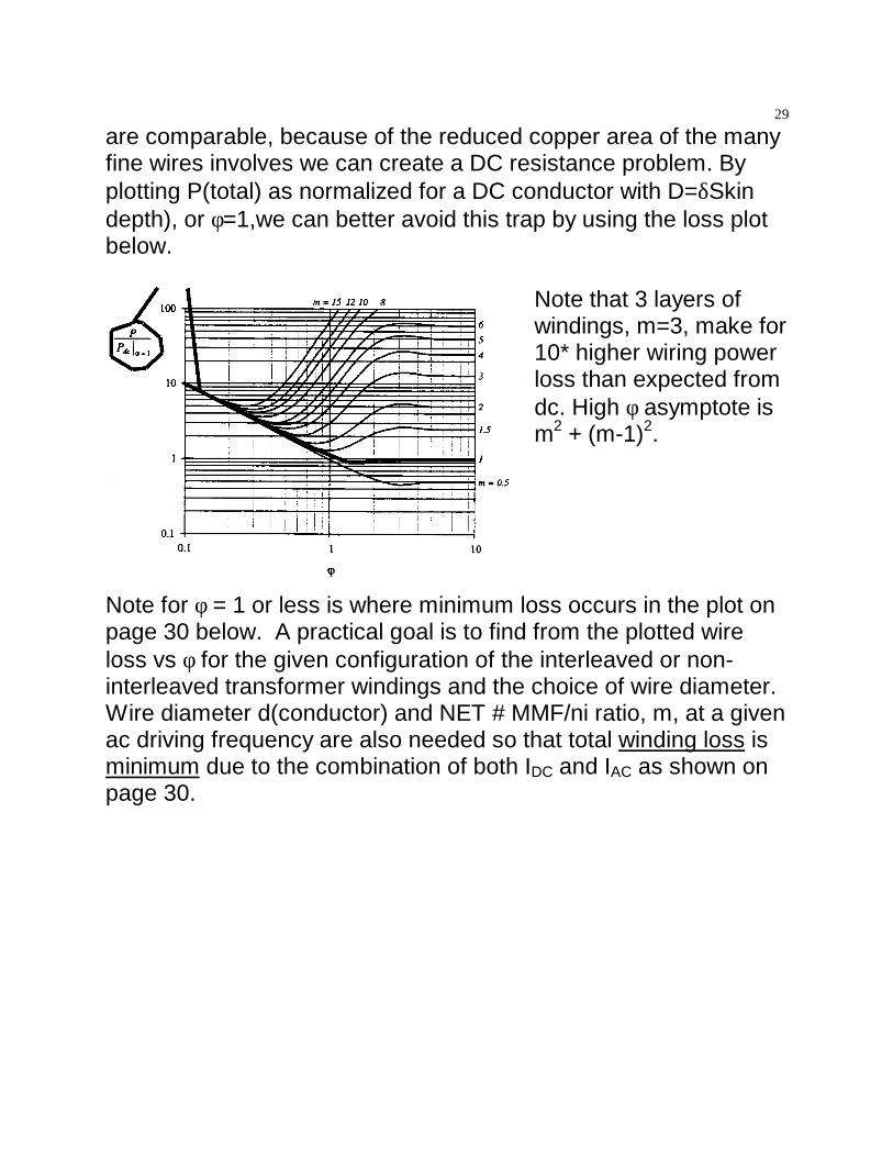
are comparable, because of the reduced copper area of the manyfine wires involves we can create a DC resistance problem. Byplotting P(total) as normalized for a DC conductor with D=δSkindepth), or φ=1,we can better avoid this trap by using the loss plotbelow.

Note that 3 layers ofwindings, m=3, make for10* higher wiring powerloss than expected fromdc. High φ asymptote ism2 + (m-1)2.

Note for φ = 1 or less is where minimum loss occurs in the plot onpage 30 below. A practical goal is to find from the plotted wireloss vs φ for the given configuration of the interleaved or non-interleaved transformer windings and the choice of wire diameter. Wire diameter d(conductor) and NET # MMF/ni ratio, m, at a givenac driving frequency are also needed so that total winding loss isminimum due to the combination of both IDC and IAC as shown onpage 30.

30

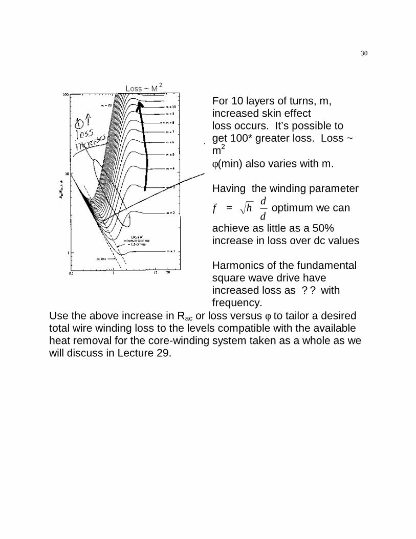
For 10 layers of turns, m,increased skin effectloss occurs. It’s possible toget 100* greater loss. Loss ~m2

φ(min) also varies with m.

Having the winding parameter

φ ηδ

= d

optimum we can

achieve as little as a 50%increase in loss over dc values

Harmonics of the fundamentalsquare wave drive haveincreased loss as ? ? withfrequency.

Use the above increase in Rac or loss versus φ to tailor a desiredtotal wire winding loss to the levels compatible with the availableheat removal for the core-winding system taken as a whole as wewill discuss in Lecture 29.