lecture 3 characterizing vegetation part 3 plants … 3 characterizing the vegetation, part ii: ......

Biometeorology, ESPM 129, Characterizing Vegetation, Part II

1

Lecture 3 Characterizing the Vegetation, Part II: Plants, Leaves and Roots Instructor: Dennis Baldocchi Professor of Biometeorology Ecosystem Science Division Department of Environmental Science, Policy and Management 345 Hilgard Hall University of California, Berkeley Berkeley, CA 94720 August 29, 2016 This set of lectures will discuss:

1. The physical characteristics of vegetation canopies a. canopy height b. leaf angle distribution, inclination and azimuth c. spatial distribution of leaves

i. projected to surface area ratios, shoots and non-flat leaves ii. clumping relations

d. basal area and woody biomass index 2. Physical characteristics of leaves and stems a. leaf anatomy

b. specific leaf area c. chemical composition of leaves, stems, roots (C/N ratios) 3. Roots

a. Rooting Depth b. soil depth and water 4. Summary L3.1 Canopy Height Canopy height is a plant structural variable that has important consequences on the biometeorological conditions of a plant canopy. Most importantly, it affects the aerodynamic roughness and reflectivity of the surface. It also has an impact on the physiological functioning of the plant by limiting water transport. Many factors affect plant height. One of the most important factors for stimulating height is competition for sunlight. Taller trees and plants are able to harvest more sunlight, giving them an advantage over their neighbors. Offsetting factors, limiting tree and plant height, include extra costs for maintenance respiration of extra supporting


2

tissue. Tall plants are vulnerable to wind throw. The transport of water and nutrients to tall plants also becomes more difficult. Tallest trees grow where water is available and there is shelter from drying and destroying winds. Trees, as tall as 45 m, inhabit the tropical forests and can reach 80 to 100 m on the Olympic Peninsula of Washington and along the California-Oregon coast.

Figure 1 Old growth redwoods (~80 m tall), Lady Bird Johnson Grove, Redwoods National Park, Orick, CA. D. Baldocchi photo.

In the literature, four theories have been debated on what limits maximum tree height (Ryan and Yoder, 1997). They include: a. respiration hypothesis: bigger trees respire more since they have more biomass (new data fail to support this hypothesis as respiration declines with a decline in growth). b. nutrient limitation hypothesis. sequestration of nutrients in biomass and detritus of old stands. This forces more below ground allocation to fine roots and limits growth. (works in some circumstances, but is not general) c. maturation hypothesis. all organisms show maturation limitations (grafting experiments show that maturation did not limit growth) d. hydraulic limitation hypothesis. stomata on older trees close earlier in the day than young trees, as older trees have a greater hydraulic resistance. Hydraulic resistance increases with tree height and sapwood permeability. Hydraulic theory explains why height is limited on nutrient poor sites and in different environments. Hydraulic


3

resistance increases with tree height and age in several studies. Stomatal conductance and photosynthesis is lower in old trees. e. wind loads. High winds will limit tree height. Trees growing in windy areas either experience windthrow or bend over; take a look at the trees growing near the Pt Reyes Lighthouse. Physics acts to limit infinite tree height, as the movement of water to great heights has many costs. The hydrostatic pressure gradient is 0.01 MPa m-1, which would institute a 1 MPa gradient between the top of a 100 m tree, without any considerations of other resistances along the transpiration pathway. To put this number in perspective, soil water deficits of about -1.5 MPa (a definition of the permanent wilting point) stress plants and limit photosynthesis. In the case of tall redwoods, a physical limitation to water transport can be overcome by the interception of fog by the trees (a theory proposed by Todd Dawson). Andrew Friend (1995) performed numerical simulations on potential tree height. He concluded that depressed water potentials and additional respiratory costs limited tree height. His computations showed that the combined effects of respiration and water transported limited tree height to about 60-70 m. Ryan et al (2006) recently revisited the hydraulic limitation hypothesis. They conclude that

Hydraulic limitation of gas exchange with increasing tree size is common, but not universal

No evidence supports the original expectation that hydraulic limitation of carbon

assimilation is sufficient to explain observed declines in wood production

Any limit in height does not appear to be related to age-related decline in wood production

A new study by Koch et al. (2004) examined gradients of water potential, stomatal conductance and carbon isotopes through the height of 100 m+ redwood trees. They did not find support for the maturation limitation theory. They found that elevation increased the gravitational water potential on leaves and imposed a leaf water stress, even when soil moisture was ample. They conclude that height is limited due to a hydraulic constraint because “water potential, turgor, leaf structure, carbon isotope composition, and photosynthesis all change with height as they do along gradients of soil moisture stress, consistent with a general role for water availability in determining leaf functional traits”.


4

Figure 2 Vertical variation of redwood leaf morphology with height. Koch et al. 2004 Nature

Another source of variation in canopy height is altitude. Data from Puerto Rico (Weaver, 1994) suggests that tree height diminishes with altitude. At 350 m trees on ridge, values and slopes range between 20 and 23 m. At 1050 m the height of trees in valleys, slopes and ridges are between 3 and 10 m. Temporal Variation Like leaf area index, canopy height of herbs will vary during the growing season as the plants grow. Herbaceous annuals start life from a seed. A soybean plant, for instance, will vary from near zero to one meter.

Figure 3 Seasonal variation of canopy height of a soybean canopy growing near Mead, NE. D. Baldocchi dissertation.

day

160 180 200 220 240 260

hei

gh

t (m

)

0.0

0.2

0.4

0.6

0.8

1.0

1.2

Clark soybeans1979, Mead, NE


5

High and low tech methods are used to measure plant height. A meter stick can be easily used to measure the height of short crops and grasses. Tree height is usually measured with a hypsometer. Tree height is determined via the trigonometric relation between the distance to the tree and the angle between the observer and the top of the tree. Pulse or wave-form recording laser altimeters mounted on helicopters, aircraft or satellites is a modern way to determine canopy height with high spatial resolution. The time history of a laser beam projected at a canopy determines the vertical distribution of illuminated foliage. The laser altimeter sends a waveform to the surface and samples its reflectance with high temporal resolution. The intensity of the backscatter received is a function of the probability that that beam can penetrate to a certain canopy depth and its reflectance can exit the canopy (Harding et al., 2001). The method has to correct for multiple scattering of laser beams in the canopy, so the method is a function of the reflectance of leaves and spatial distribution of leaves. Laser altimeters can be used to characterize tree height across a transect if mounted on an aircraft or helicopter.

Figure 4 Tramsect of tree height at the Wind River Crane Field site, an old growth Douglas fir forest. (Lefsky et al., 2002)

Or with the use of a crane system, it can produce high detailed 3-D information on stand structure, showing shapes of crowns and gaps between trees, as shown in Figure 5.


6

Figure 5 from Lefsky et al 2001

Scientists are also using synthetic aperture radar to study the vertical structure of plant canopies (Harding et al., 2001). SAR polarimetry is sensitive to the shape and orientation of vegetation, while interferometry is sensitive to the spatial separation of foliage elements. Polarmetric systems can probe a deep canopy, but the intensity and polarization of the reflected radar is a complex function of wavelength dependent scattering by leaves, branches and trunks (Harding et al. 2001). Radar method are still under development and at present has an error of about 4.0 m, which is a considerable fraction of forest vegetation 20 m tall. With this new pulsed laser technology, we recently acquired a LIDAR scene for the oak savanna we are studying near Ione, CA.


7

Figure 6 3-d map of an oak savanna ecosystem near Ione, CA. the scale is 1 km by 1 km. Data of Qi Chen and D. Baldocchi.

L4.2 Leaf Inclination Angle Distribution Walking through a forest, one will readily observe that leaves have no preferred orientation. Some point west, others north, south and east. Some are flat and others are pointing towards the sun (Falster and Westoby, 2003; Hutchison et al., 1986) (see Figure 6 and Table 1).


8

Figure 7 Cumulative area-weighted frequency distribution of the inclination angles of leaves in three major stata of a deciduous forest in eastern Tennesssee, USA. After Hutchison et al. 1986

Table 1 List of leaf angles on sun and shaded leaves (adapted from (McMillen and McClendon, 1979).

Species Sun leaves Shade leaves Cottonwood 75 32 Redbud 36 14 Green ash 37 14 Red oak 10 11 Sugar maple 15 8 Crop breeders have exploited interrelationships between leaf angle and light interception to breed plant lines with erect leaf orientations; notice the very erect corn fields growing in the Central Valley. Model calculations show that canopies with erect leaves are the most productive. I have performed similar calculations for canopy photosynthesis of oak and find that net productivity is indeed greatest for canopies with erect leaves (Table 2).

Table 2 Annual sums of net CO2 exchange as a function of leaf inclination angles and clumping. We assumed the mean angle for the erect canopy was 80 degrees and it was 10 degrees for the plane canopy. The mean direction cosine between the sun and the leaf normal is 0.5 for the spherical case.

clumped random spherical erectophile planophileNEE (gC m-2 a-1) -577 -354 -720 -1126 -224 But in nature we rarely see natural forest stands with erect leaves (Table 1). Plants need to out-compete their competitors. Allowing more light to penetrate deep into a plant


9

canopy has the potential to aid the production of inferior plants, which may grow up and over the dominant plants with erect leaves and shade them instead. One measure of the distribution function of foliage area orientation is the leaf normal distribution function, g (Ross, 1980). This function that quantifies the probability of the leaf normal within the solid angle around a direction, r, such that

If the leaves are azimuthally symmetric then we define the distribution function, g, as the probability that leaves that the leaf angle is a certain value, which must sum to one:

g dL L( )/

0

21z

Conceptually, these equations define a histogram of leaf angles as a function of azimuth and elevation angle. Several general classes of leaf inclination have been reported in the literature (Lemeur and Blad, 1974; Norman and Campbell, 1989; Ross, 1980). Erectophile, plagiophile, spherical, and planophile are the types most commonly reported. At the name suggests, erectophile canopies possess a disproportionate fraction of erect leaves. In contrast, a planophile canopy possesses mostly flat leaves. The spherical distribution is envisioned by the surface of a basketball. If one plucks leaves and keeps their azimuth and elevational angles, one will soon cover the surface of that ball. Leaf angles are easily measured with a compass and protractor. In a plagiophile canopy, leaves are most frequent at an oblique inclination and extremophile leaves are least frequent at oblique inclinations. A visual representation of the probability distributions that are produced with these equations is shown below.

1

21

0

2

0

2

d g dL L L L( , )/zz


10

Figure 8 Leaf inclination angle distribution for three leaf angle classes.

Another way to look at leaf angles is to examine their cumulative distribution.

Figure 9 Cumulative leaf angle distribution

leaf angle

0 20 40 60 80

f(

0.000

0.005

0.010

0.015

0.020

0.025

0.030

0.035

0.040

planophile

erectophile

extremophile

leaf angle distribution functions

Leaf Angle

0 20 40 60 80

Cum

ulat

ive

Ang

le D

istr

ibut

ion

0.0

0.2

0.4

0.6

0.8

1.0

planophileErectophileExtremophile


11

In this manner, the mean leaf angle corresponds with 50% on the cumulative distribution. So a planophile canopy has a mean angle of about 20 degrees and an erect canopy has a mean angle of about 70 degrees. Native stands tend not to possess constant leaf angles through the canopy. The forest we worked at in Oak Ridge, TN possesses relatively erect leaves near the top of the canopy (mean angle of about 40 degrees) and very horizontal leaves near the forest floor. This configuration is a more efficient way to capture light.

Figure 10 Flat leaves in the understory of a temperate forest.

Other types of vegetation possess heliotropic leaves, ones that track the sun. Sunflower is a prime example. If the plants are heliotropic or if their leaf distribution is asymmetrical, data on the azimuthal orientation of leaves is needed (Lemeur and Blad, 1974); sunflower, Jerusalem artichoke, corn, soybeans, Quercus coccifera are examples of crops and trees that exhibit asymmetry in their leaf azimuthal distribution (Lemeur, 1973); Long term exposure also affects leaf angle orientation (Figure 10). In canopies with low leaf area index, most leaves are exposed to ample sunlight. Falter and Westoby (2003) report that it is more important to maintain steep leaf angles to reduce exposure to excess light than to maximize solar interception to maximize carbon gain (this is especially true in water limited environments like Australia.


12

Figure 11 Falster and Westoby 2003

L4.3 Spatial Distribution of Leaves and Plants Plant display leaves in various spatial dispersion patterns (Figure 11). Four types of interest include:

1) regular; 2) semi-regular; 3) random and 4) clumped. Regular dispersion is observed in the deliberate spacing of orchards. Row crops tend to have semi-regular spacing as seeds may not be regularly dropped, but they maintain definite row spacing. Broadcasted crops are random. Natural stands tend to have clumped distributions, due to the competition, seed dispersal and mortality effects.


13

Figure 12 Spatial distribution of plants

The relative variance ( x

x

2

) is zero for a regular distribution, between zero and one for a

semi-regular distribution. The relative variance is one for a random distribution and greater than one for a clumped distribution (Nilson, 1971). Vegetation in semi-arid regions can possess regular and irregular patterns. The Tiger bush in Niger, is an example of a regular pattern, as are row crops (Figure 11). Stripes of alternating lines of vegetation and bare soil are established because slight slopes and impermeable soils cause rain to drain to where plants exist and infiltration is better. The plants exhaust water on the 'uphill' side, causing another bare stripe to initiate.

Regular Clumped

Quasi-regular Random


14

Figure 13 Tiger Bush, Sahel Africa http://www.geog.ucl.ac.uk/~mdisney/ASAS.sss_30.sep17_92.301.r1.tilt6.refl.band_2.gif

Probability statistics are used to predict where plants may exist is a domain. A random distribution occurs if the position of a plant does not affect the position of the next plant. This condition is not the case for a regular, row spaced crop. The Poisson distribution is used to compute the probability that a space will be free of plants:

Pn

nnplants n

plants( ) ( ) exp( )0 1

where np is the number of plants per square meter. Markov or negative binomial distributions are invoked for clumped distributions. The same concepts of random, regular and clumped distributions are valid for the spatial array of leaves within the crown of a plant. We will exploit this concept more at a later date when we discuss photon transport through vegetation. L4.3.1 Arrangement at the shoot level Conifer trees display their 'leaves' as needles on shoots. Conifers are able to maintain higher leaf area indices than would be possible if they possessed flat leaves. The mutual shading of needles on a shoot cause the ratio of shoot silhouette area to needle area to be less than one (in contrast this 'ratio' would equal one for a flat leaf). The shoot silhouette to total needle surface area (STAR) is a measure of shoot geometry and is an index from which to calculate light capture efficiency. Conifers are able to maintain high leaf areas for the shoots are able to capture sunlight efficiently (Stenberg, 1996). STAR depends on shoot structure and view angle, relative to the light source.


15

Figure 14 Actual and projected shoots

Mathematically this relation can be expressed as:

STARA

Ad dsilhouette

needle

zz1

2 00

2 2

( , )sin

The needle area is the all-sided needle area

Table 3 Common STAR values for conifers. after Stenberg (1996)

Species STAR, average Pinus sylvestris 0.135-0.163 Pinus contorta 0.1160 Picea abies 0.161-.216 The importance of evaluating STAR at a variety of angles, rather than from the zenith, as had been done in many prior studies is illustrated in Figure 14.


16

Figure 15 Silhouette of ponderosa pine shoot at azimuth of 0 and shoot angels of 0, 45 and 90 degrees (Law et al., 2001).

Care must be exercised when conducting or interpreting such measurements. Some investigators normalize the projected shoot area by the projected area of needles, others use the half or total surface area of needles. The ratio of total needle area to silhouette area is a factor of pi, 3.1415. This issue is discussed further in the next section.

L4.3.2 Needles and Non-Flat Leaves The amount of leaf area on a needle (on a ground area basis) is greater than that of a flat leaf. In many applications it is important to distinguish the differences between one-sided, projected and total leaf area of needles. Radiation interception is related to one sided, and the resulting shadow relates to projected area. Mass and heat exchange area affected by total area. Many workers define leaf area index for conifers and non flat leaves as one-half the total leaf area per unit ground area. Lang (1991) revisited Cauchy's theorem to assess the leaf area of non-flat surfaces. Cauchy wrote in 1832 that the average silhouette of a convex solid was ¼ of the surface area for any body shape. Using light transmission theory, Lang (1991) defines G as the ratio of the silhouette to plan area of a leaf. For flat leaves G is ¼ for total surface area and ½ for the plan area. For convex solids, Lang defines H, the ration of the silhouette area to surface area. Integrating H with respect to view angle yields ¼. To avoid ambiguity, Lang recommends that we state areas with respect to surface area. Chen and Black (1992) report that the mean area projection coefficient based on one half the total surface area is 1/2 for shapes such as spheres, circular cylinders, hemi-circular cylinders, bent plates and multi-sided bars. So in other words the leaf area index of non-flat leaves should be approximated as one-half the intercepting area per unit ground area. The simplest example of this behavior can be demonstrated by comparing the projected area of a sphere (Ap, the area of a circle) and the integrated surface area of the sphere:

A

A

r

rp

2

24

1

4

If we consider a hemisphere, then the ratio is ½.


17

Most needles have non-ideal shapes. Consequently, the volume displacement method is used to estimate the one half total needle area of a conifer shoot. L4.4 Leaf Anatomy If we are to study trace gas exchange to and from leaves, we must have a basic understanding of the anatomy of a leaf and the pathway which gases will travel. A leaf consists of three tissue types. These are epidermal, mesophyll and vascular. The basic features of the cross section of a leaf consists of the external cuticle, an upper and lower epidermis, palisade mesophyll, spongy mesophyll, stomata and intercellular space (Nobel, 1999). The stomata consist of the stomatal pore, guard cells and subsidiary cells. Leaves tend to be about 4 to 10 cells or 50 to 200 m thick. Mesophyll cells contain chlorophyll and are capable of photosynthesis. The cytoplasm of a chlorenchyma cell includes chloroplasts, mitochondria, endoplasmic reticulum, peroxisomes, vacules, etc. Leaves may be hypostomatous (having stomata on one side) or amphistomatous (having stomata on both sides of the leaf. This distinction is very important when we evaluate rates of leaf gas exchange. Amphistomatous leaves tend to be associated with thicker leaves, and ones with higher photosynthetic capacity, full sun and inhabiting habitats with adequate soil moisture, as this morphology is needed to facilitate diffusion into the leaf.

Figure 16 Cross section of a leaf with the C3 photosynthetic pathway

WaxyCuticle

UpperEpidermis

PalisadeParenchyma

SpongyMesophyl

Guard Cells Sub stomatal Cavity


18

With regards to mass and energy exchange, water vapor originates from the inner side of the guard cells and from the subsidiary cells. CO2 diffuses across the intercellular air space of the mesophyll. Representative mesophyll thickness of 200 um, air space volume of 30%. C4 leaves, in contrast, have Krantz anatomy. Leaves of this type possess bundle sheaths. Corn is an example of this morphotype.

Figure 17 www.agen.ufl.edu/.../ lect/lect_15/lect_15.htm

Leaf architecture is affected by several environmental factors. The most important factors are exposure of the leaf to sun or shade. Sun leaves are thicker than shade leaves, have greater specific mass and a higher stomatal density than shade leaves (Nobel, Abrams and Kubiske, 1990, Forest Ecology and Management, 31: 245-253. One measure of leaf anatomy is the leaf mesophyll area to surface area ratio (Nobel, 1999). The mesophyll area represents the amount of mesophyll exposed to intercellular air spaces. The ratio of mesophyll area to surface area is important for converting the cellular resistance of CO2 transport to that for the leaf mesophyll:

rr

AA

mesophyllcell

mesophyll


19

Typical values for the Ameso/A range between 10 to 40 for mesophytes. One survey of twelve species showed that, on average Ameso/A is about 31 for C3 species. In contrast, Ameso/A is about 16 for C4 species. Extreme values are limited by the diffusion of CO2 through the mesophyll to chloroplasts and the interception of sunlight. Ameso/A is two to four times greater for sun leaves than for shade leaves. For example, Fragaria vesca for instance increased from about 10 to 25 as PAR increased from near zero to 30 mol m-2 day-1. Low soil water potential leads to smaller leaves, though not necessarily Ameso/A (Nobel, 1990). In essence, there are physical limits on the thickness of leaves due to limitations in the diffusion of CO2 and the transmission of light through the mesophyll. As leaves get thicker and thick more photons are intercepted (see Fig 16). If the leaf is so thick that all photons are intercepted above a certain layer, there is no energy to drive photosynthesis, hence no reason and ability to sustain additional layers of mesophyll cells. Similarly if leaves are so thick, most the CO2 will be scrubbed before it can reach cells deep within the mesophyll.

Figure 18 Theoretical profiles of gas exchange across leaves. (Ustin et al., 2001)

L4.3.1 Specific Leaf Weight Rubisco, the photosynthetic enzyme, is composed of nitrogen. Leaf mass per unit area and Nitrogen per unit area are well correlated and vary with height in the canopy; it is not economic to allocate expensive resources deep in the canopy where they are not needed. The correlation between leaf mass per unit area and N reflect differential and plastic adaptations among sun and shade leaves to harvest sunlight.

0 20 40 60 80 100

-150

-100

-50

0

Relative net flux

Le

af

de

pth

epidermis

0 0.2 0.4 0.6 0.8

Photosynthesis

palisade parenchyma

spongy mesophyll

epidermis

0 500 1000 1500 20000

2

4

6

Irradiance

Ph

oto

sy

nth

es

is


20

N (g m-2)

0.5 1.0 1.5 2.0 2.5 3.0

leaf

mas

s p

er u

nit

are

a (L

MA

) (g

cm

-2)

0.002

0.004

0.006

0.008

0.010

0.012

0.014

Figure 19 Profile of leaf mass per unit area of a Quercus alba in broadleaved forest and leaf nitrogen. (Wilson et al., 2000).

Upper leaves are thicker and have more mass per unit area, than leaves in the understory that are thinner and wider, so we observe a strong vertical gradient in photosynthesis with height. They also have more N per unit leaf area. Inversely, leaves deep in the canopy are shade adapted so they need to be broader, per unit mass to capture light more efficiently, which increases their leaf area to mass ratio and decreases their mass to area ratio. If we multiply typical vertical gradients of N (mass per area) vs leaf area to mass ratios, we observed that leaf N on a mass per mass basis (mg/g) is rather conservative with height (for a temperate forest N was 2.1 mg g-1 +/- 0.2).

Across ecosystems, these simple relationships break-down and are replaced by others, whose constraints are set by biophysics and natural selection lead to compromises in leaf structure and function. Reich et al. (1997) found that the potential for carbon gain and loss increase in proportion with decreasing life span, increasing leaf nitrogen concentration and increasing leaf surface area to mass ratio.


21

Leaf N (mg g-1)

1 10 100

A (m

ol g

-1 s

-1)

10

100

Lifespan (months)

1 10 100

10

100

Specific Leaf Weight (m2 g-1)

10 100 1000

Le

af N

(m

g g

-1)

1

10

100

Lifespan (months)

1 10 1001

10

100

adapted from Reich et al. 1997, PNAS, Figure 20 Relations between leaf nitrogen, photosynthesis, specific leaf weight and lifespan. (Reich et al., 1997) .

(the work of Reich et al, was recently expanded in a review of data for 700+ species by Wright et al (Wright et al., 2005). They reported that 82% of variation was explained by 3 way interaction among photosynthesis per unit mass (Amass), specific leaf weight (area per unit mass) and leaf nitrogen per unit mass Nmass). The global syntheses of leaf traits indicate that there is coordination among leaf traits is stronger on a mass basis than a leaf area basis. Conceptually (from a physiological and physic perspective), high photosynthetic rates per unit mass (Amass) requires high high level of nitrogren, per unit mass (Nmass). But this requirement leads to vulnerability of herbivory and more respiration, which places limits on specific leaf weight. Leaf longevity is correlated with specific leaf weight because longer living leaves must be tougher and have low palatability. Climate effects were found to be weak. The information in Figure 21 lead Reich et al to develop several Corallaries:


22

1. There are no species with thin, short-lived leaves and low Amax. This is because the combination of low photosynthetic capacity and a short growing season leads to low summations of net primary productive. The behavior does not offset respiratory costs well. 2. There are no thick, dense and long-lived leaves with high mass-based N, Amax and Rd values. Several factors lead to this exclusive combination. Thick and dense leaves lead to within leaf shading and diffusion limitations. Leaves with high N suffer from herbivory, which limits longevity. High Amax is associated with fast growing species, so this is not an optimal allocation of resource for long lived species. Slow growing plants live in low light and low N environments and will not benefit from traits that allow high growth. Niinements (2001) discusses a contradiction between photosynthesis and leaf size, as expressed on a mass or area basis. Many field studies show a negative correlation between photosynthesis on a unit mass area with LMA, leaf dry mass per unit area (and a positive correlation between photosynthesis per unit mass and specific leaf weight (area per unit mass). Niinemets discusses how LMA is a product of leaf density and thickness, and concludes that Amax scales positively with leaf thickness, but is negatively correlated with leaf density:

“ thicker leaves have more photosynthetic machinery; denser leaves exert more resistance to gas phase transfer of CO2.”

Another issue associated with the perceived contradictions is that Reich’s et al relationship that photosynthesis per unit mass correlates well with specific leaf weight across ecological gradients, where there are gradients in N (mg/g). On the other hand, within a canopy there seems to be a strong relationship between photosynthesis per unit area and specific leaf weight because N is relatively constant with depth, but leaf mass per unit area decreases with depth into the canopy. Niinemets makes it clear from his analysis that thick leaves are an important attribute of plants in hot climates with ample sunshine. Thick leaves are able to better utilize the available energy for photosynthesis. Where water is limited, there is a tendency for plants to grow dense leaves. These leaves tend to be longer living and possess lower photosynthetic rates. More recently, Farquhar et al (2002) reported links between rainfall and leaf N. These data are consistent with our findings that Q. douglasii have very high leaf N, thick leaves and high photosynthetic capacity in able to acquire enough carbon to sustain their respiratory cost in an environment with low rainfall and high potential evaporation. (they examined if optimization changes with water supply. Farquhar conclude that:


23

“ our… analysis suggests that as conditions become more arid, there should be both a smaller stomatal conductance and less leaf area with greater nitrogen per unit area.”

Figure 21 From Farquhar et al. 2002

L4.4 Roots Roots are a major conduit for the transfer of water, nutrients and carbon between the soil and atmosphere. They take up water and nutrients from the soil and transfer hormonal signals (ABA), which are known to regulate stomata. Though deep taproots are noted in many species, until recently it has been conventional wisdom that the majority of roots were located in the top meter of soil where there is plenty of nutrients, microbes, oxygen and water. Recent surveys on root distributions across the globe are shedding new light on the where roots are located (Canadell et al., 1996; Jackson et al., 1996). These deep roots, though a small proportion of total root mass play important roles in the functioning and existence of various plant species and functional types. For example, primary productivity can occur in dry climates when plants can tap deepwater sources. Rooting depth also seems to be a factor in delimiting the boundary or co-existence of evergreen and deciduous species. There is also a feedback between rooting depth, available water source, stomatal conductance, evaporation and regional hydrology ((Kleidon and Heimann, 1998). Typically over 90% of root biomass is in the top meter of soil. Yet, many plant species exist which possess roots down to 10 m. The deepest roots are on the order of 50 m.


24

To fully understand the role of roots and how deep they may go we also need to know about depth to bedrock, soil texture, water holding capacity, water logged areas. Jackson et al. developed an analysis of the cumulative root fraction with depth

Y=1-z Beta values approaching one correspond with a root depth distribution that places more roots at depth. Beta values less than one yield cumulative distributions that have the majority of roots close to the surface. The exponent z is depth in centimeters. Tundra, boreal forests and grasslands have the shallowest roots ( equal 0.913, 0.943, 0.943, respectively). Deserts, temperate coniferous forests and savanna have the deepest roots. In general, tundra have 60% of of their roots in top 10 cm, as deep soils are often frozen. On the other hand, desert species have only 20 % of roots in top 10 cm. Instead they can have roots as deep as 53 m, as needed to tap distributed water sources.

Table 4 Model parameters on cumulative root distribution (Y=1-n) After Jackson (1999).

biome total roots % roots in upper 30 cm

fine roots % roots in upper 30 cm

boreal forest 0.943 83 .943 83 desert 0.975 53 .97 60 sclerophyllous shrubs

0.964 67 .95 79

temperate conifer forest

0.976 52 .98 45

temperate deciduous forest

0.966 65 .967 63

temperate grassland

0.943 83 .943 83

tropical deciduous forest

0.961 70 .982 42

tropical evergreen forest

0.962 69 .972 57

tropical savanna 0.972 57 .972 57 tundra 0.914 93 .909 94 Information on maximum rooting depth is important for a disproportionate amount of water uptake may be associated with deep roots, which are a small fraction of total roots. In one study, over one-half of water uptake was from roots below 60 cm, which were only 20% of root biomass, and 20% of water uptake came from roots below one meter, which were less than 3% of the roots (Gregory et al., 1978). For deep roots to be functionally important:


25

1. vegetation must be capable of growing deep roots. 2. roots must be able to penetrate soil. 3. deep soils must hold worthwhile resources. As we will discuss later, it is important to know the vertical distribution of roots (r) in order to compute weighted and integrated estimates of soil moisture () and temperature that is relevant to the process under examination.

zz

( ) ( )

( )

z r z dz

r z dz

z

Z0

0

L4.5 Summary

Temporal and spatial variations in canopy structure (e.g. leaf area index, species, leaf inclination angles, leaf clumping) and function (e.g. maximal stomatal conductance, photosynthetic capacity) modulate trace gas fluxes by altering: 1) wind and turbulence within and above the canopy; 2) the interception and scattering of photons throughout the canopy; 3) the heat load on leaves and the soil; 4) the physiological resistances to water and CO2 transfer and 5) the biochemical capacity to synthesize or consume carbon dioxide.

This lecture focused on the following plant attributes: tree height, leaf angles,

spatial distribution of leaves and plants, leaf anatomy and roots.

Plant height affects the aerodynamic roughness of the canopy, the ability to transfer water from the roots to the leaves and alters the ability of a canopy to trap light. New technology based on laser altimeters mounted on aircraft is giving us a new way to visualize and quantify the height and its variability in tall forests. Tree height is limited by a combination of physical limits to transfer water to great heights and the metabolic costs of support biomass to do this.

Leaf inclination angles have a major impact on light transmission through plant

canopies and can have major impacts on net primary productivity. Leaf angles of plants vary due to natural selection, light acclimation and genetic breeding. Leaves deep in the canopy tend to be horizontal, while those near the top are more erect.

How leaves and plants are distributed spatially affects turbulent mixing and light

transmission. Leaves that are clumped allow light to be transmitted deeper into the


26

canopy. Field and modeling studies show this attribute is extremely important, but one often overlooked by practitioners.

Leaf anatomy is a function of photosynthetic pathway (functional type) and

acclimation. Leaves near the top of the canopy are thicker where they tend to be sunlit than those near the bottom, which tend to be shaded. There are physical limits to leaf thickness. Its importance affects micrometeorology, plant physiology and isotope biogeochemistry.

Global surveys on leaf properties show a positive correlation between

photosynthesis per unit mass and leaf nitrogen and in inverse relation with leaf longevity.

New global surveys on root distributions of plant functional types have been

produced. This information is needed to study the mining of soil moisture by plants. It is also needed to determine weighted measures of soil moisture, soil temperature and the production of CO2.

Table 1 presents a summary of key leaf and plant characteristics, their attributes

and how these two features impact mass and energy exchange of plant canopies and affect the local microclimate.

Table 5 Structural and functional attributes of leaves, plants and plant stands and their impact on carbon, water and energy fluxes (Baldocchi et al., 2002; Horn, 1971; Nobel, 1999; Norman and Campbell, 1989; Ross, 1980). Ga: aerodynamic conductance; Gs: surface conductance; P(0): light transmission through a leaf or canopy; : albedo or reflectivity; Ci: biochemical capacity

Characteristic Structural or Functional Attribute

Primary Impacts on Carbon, Water and Energy Fluxes

Leaves Photosynthetic pathway C3,C4,CAM, maximal stomatal

conductance Ci , Gs

Leaf size/shape Needle/planar/ shoot; projected/surface area, penumbra/umbra

Ga, P(0)

Leaf inclination angle distribution

Spherical, erectophile, planophile

P(0)

Leaf azimuthal angle distribution

Symmetric/asymmetric P(0)

Exposure Sunlit/shaded; acclimation Ci, Gs, Optical properties Reflectance,transmittance,

emittance

Leaf thickness Photosynthetic capacity, supply of CO2 to chloroplast, optical

Ci ,Gs,


27

properties, Stomatal conductance capacity

Stomatal distribution Amphistomatous/hypostomatous Gs Plants/Trees Crown volume shape Cone, ellipse, cylinder P(0), Ga Plant species monoculture, mixed stand,

functional type P(0), Ga, Gs, Ci

Spatial distribution of leaves

Random, clumped, regular P(0)

Plant habit Evergreen/deciduous; woody herbaceous; annual/perennial

Ga, Gs,

Plant height Short (< 0.10 m) tall (> 10 m)

Ga,

Rooting depth Accessible water and nutrients, plant water relations

Gs

Leaf area/sapwood ratio Hydraulic Conductivity Gs, Ci

Forest Stand Leaf area index Open, sparse, closed P(0), Gs, Ga Vertical distribution of LAI Uniform, skewed Ga, P(0) Seasonal variation of LAI Evergreen/deciduous; winter or

drought deciduous Ga, Gs

Age structure Disturbed/undisturbed; plantation; agriculture; regrowth

Ga, Gs, P(0)

Stem density Spatial distribution of plants Ga, Woody biomass index Amount of woody biomass Ga, P(0) Topography Exposure, site history, water

balance Ga, Gs

Site history Fires, logging, plowing, re-growth

Ga,Gs,Ci,

As we walk through the country-side it become readily obvious that different types of ecosystems, growing in different climates have different structural properties. To get a sense of how micrometeorological and plant canopy attributes of different ecosystems compare, we draw on compiled lists by the author and assorted references (Breuer et al., 2003; Myneni et al., 1997; Saugier et al., 2001).


28

Table 6 Summary of Plant Attributes

Parameter grass/ cereal

shrub Broad-leaved crop

savanna Broad-leaved forest

needle leaved forest

LAI 0-5 1-7 0-6 0-7 3-7 1-10 fraction of ground cover

1.0 0.2-0.6 0.1-1 0.2-0.4 >0.8 >0.7

understory LAI

- - - 0-5 0-2 0-2

leaf normal orientation

erectophile

uniform uniform uniform/erectophile

uniform/ planophile/ clumped

uniform/ planophile/ clumped

fraction of stems

- 0.05 0.10 0.10 0.15-20 0.15-0.20

leaf size (m) 0.05 0.05 0.10 0.10 0.10 0.01 crown size 4 by 4 10 by 10 7 by 7

Table 7 Survey of Biophysical parameters, Saugier et al. 2001, Breuer et al. 2003. zo is aerodynamic roughness length.

biome albedo Height (m) Zo(m) LAI max Rooting Depth

Tropical forests

0.12-0.14 30-50 2-2.2 4-7.5 1-8

Temperate forests

0.1-0.18 15-50 1-3 3-15 0.5-3

Boreal forests 0.1-0.3 2-20 1-3 1-6 0.5-1 Arctic tundra 0.2-0.8 < 0.5 < 0.05 0-3 0.4-0.8 Mediterranean shrubland

0.12-0.2 0.3-10 0.03-0.5 1-6 1-6

Crops 0.1-0.2 variable variable 4 0.2-1.5 Tropical savanna

0.07-0.4 0.3-9 variable 0.5-4 0.5-2

Temperate grassland

0.15-0.25 0.1-1 0.02-0.1 1-3 0.5-1.5

desert 0.2-0.4 < 0.5 < 0.05 1 0.2-15 - -


29

Table 8 Ecophysiological Parameters by Biome, Saugier et al. 2001., Breuer et al., 2003, gs is stomatal conductance, ga is aerodynamic conductance, RUE is radiation use efficiency for photosynthesis.

biome Max gs ga Max CO2 flux, day

Max CO2 flux, night

RUE

Units mol m-2 s-1 mol m-2 s-1 mol m-2 s-1 mol m-2 s-1 G(DM)/ MJ (PAR)

Tropical forests

0.5-1 0-4 -25 5-8 0.9

Temperate forests

0.5 1-4 -25 1-6 1

Boreal forests 0.2 10 -12 0-4 0.3-0.5 Arctic tundra -0.5 to -2 1-2 Mediterranean shrubland

0.5-1 -12 to -15 6-7

Crops 1.2 1-3 -40 2-8 1-1.5 Tropical savanna

0.2-1 0.1-4 -4 to -25 2-5 0.4-1.8

Temperate grassland

0.4-1 0.2-1.5 -13 to -20 0.5-4

Having a general knowledge of these features will be critical later in the course when we draw on these features to compute rates of transpiration, evaporation and photosynthesis. Endnote References Baldocchi, D.D., Wilson, K.B. and Gu, L., 2002. Influences of structural and functional

complexity on carbon, water and energy fluxes of temperate broadleaved deciduous forest. Tree Physiology., 22: 1065-1077.

Breuer, L., Eckhardt, K. and Frede, H.-G., 2003. Plant parameter values for models in temperate climates. Ecological Modelling, 169(2-3): 237-293.

Canadell, J. et al., 1996. Maximum rooting depth of vegetation types at the global scale. Oecologia, 108(4): 583-595.

Chen, J.M. and Black, T.A., 1992. Foliage Area and Architecture of Plant Canopies from Sunfleck Size Distributions. Agricultural and Forest Meteorology, 60(3-4): 249-266.

Falster, D.S. and Westoby, M., 2003. Leaf size and angle vary widely across species: what consequences for light interception? New Phytol, 158(3): 509-525.

Farquhar, G.D., Buckley, T.N. and Miller, J.M., 2002. Optimal Stomatal Control in Relation

to Leaf Area and Nitrogen Content. Silva Fennica, 36: 625–637.


30

Harding, D.J., Lefsky, M.A., Parker, G.G. and Blair, J.B., 2001. Laser altimeter canopy height profiles: methods and validation for closed-canopy, broadleaf forests. Remote Sensing of Environment, 76(3): 283-297.

Horn, H.S., 1971. The Adaptive Geometry of Trees. Princeton Univeristy Press, 144 pp. Hutchison, B.A. et al., 1986. The Architecture of a Deciduous Forest Canopy in Eastern

Tennessee, USA. Journal of Ecology, 74(3): 635-646. Jackson, R.B. et al., 1996. A global analysis of root distributions for terrestrial biomes.

Oecologia, 108(3): 389-411. Kleidon, A. and Heimann, M., 1998. Optimised rooting depth and its impacts on the

simulated climate of an Atmospheric General Circulation Model. Geophysical Research Letters, 25(3): 345-348.

Koch, G.W., Sillett, S.C., Jennings, G.M. and Davis, S.D., 2004. The limits to tree height. Nature, 428: 851-854.

Lang, A.R.G., 1991. Application of some of Cauchy's theorems to estimation of surface areas of leaves, needles and branches of plants, and light transmittance. Agricultural and Forest Meteorology, 55(3-4): 191-212.

Law, B.E., Van Tuyl, S., Cescatti, A. and Baldocchi, D.D., 2001. Estimation of leaf area index in open-canopy ponderosa pine forests at different successional stages and management regimes in Oregon. Agricultural and Forest Meteorology, 108(1): 1-14.

Lefsky, M.A., Cohen, W.B., Parker, G. and Harding, D.J., 2002. Lidar remote sensing for ecosystem studies. BioScience, 52: 19-30.

Lemeur, R., 1973. A method for simulating the direct solar radiation regime in sunflower, jerusalem artichoke, corn and soybean canopies using actual stand structure data. Agricultural Meteorology, 12: 229-247.

Lemeur, R. and Blad, B.L., 1974. A critical review of light models for estimating the shortwave radiation regime of plant canopies. Agricultural Meteorology, 14(1-2): 255-286.

McMillen, G.G. and McClendon, J.H., 1979. Leaf Angle - Adaptive Feature of Sun and Shade Leaves. Botanical Gazette, 140(4): 437-442.

Myneni, R.B., Nemani, R.R. and Running, S.W., 1997. Estimation of global leaf area index and absorbed par using radiative transfer models. Ieee Transactions on Geoscience and Remote Sensing, 35(6): 1380-1393.

Niinemets, U., 2001. Global-scale climatic controls of leaf dry mass per area, density, and thickness in trees and shrubs. Ecology, 82(2): 453-469.

Nilson, T., 1971. A theoretical analysis of the frequency of gaps in plant stands. Agricultural Meteorology, 8: 25-38.

Nobel, P.S., 1999. Physicochemical and Environmental Plant Physiology. Academic Press, 473 pp.

Norman, J.M. and Campbell, G.S., 1989. Canopy Structure, Plant Physiological Ecology. Reich, P.B., Walters, M.B. and Ellsworth, D.S., 1997. From tropics to tundra: Global

convergence in plant functioning. PNAS, 94(25): 13730-13734. Ross, J., 1980. The Radiation Regime and Architecture of Plant Stands. Dr. W Junk, The

Hague. Ryan, M.G., Phillips, N. and Bond, B.J., 2006. The hydraulic limitation hypothesis

revisited. Plant, Cell and Environment, 29(3): 367-381.


31

Ryan, M.G. and Yoder, B., 1997. Hydraulic limits to tree height and tree growth. BioScience, 47: 235.

Saugier, B., Roy, J. and Mooney, H., 2001. Estimations of global terrestrial productivity: converging toward a single number. In: B.S. J Roy, HA Mooney (Editor), Terrestrial Global Productivity. Academic Press, pp. 543-557.

Stenberg, P., 1996. Simulations of the effects of shoot structure and orientation on vertical gradients in intercepted light by conifer canopies. Tree Physiology, 16(1-2): 99-108.

Ustin, S.L., Jacquemoud, S. and Govaerts, Y., 2001. Simulation of photon transport in a three-dimensional leaf: implications for photosynthesis. Plant Cell Environ, 24(10): 1095-1103.

Wilson, K.B., Baldocchi, D.D. and Hanson, P.J., 2000. Spatial and seasonal variability of photosynthesis parameters and their relationship to leaf nitrogen in a deciduous forest. Tree Physiology., 20: 565-587.

Wright, I.J. et al., 2005. Assessing the generality of global leaf trait relationships. New Phytologist, 166(2): 485-496.


32

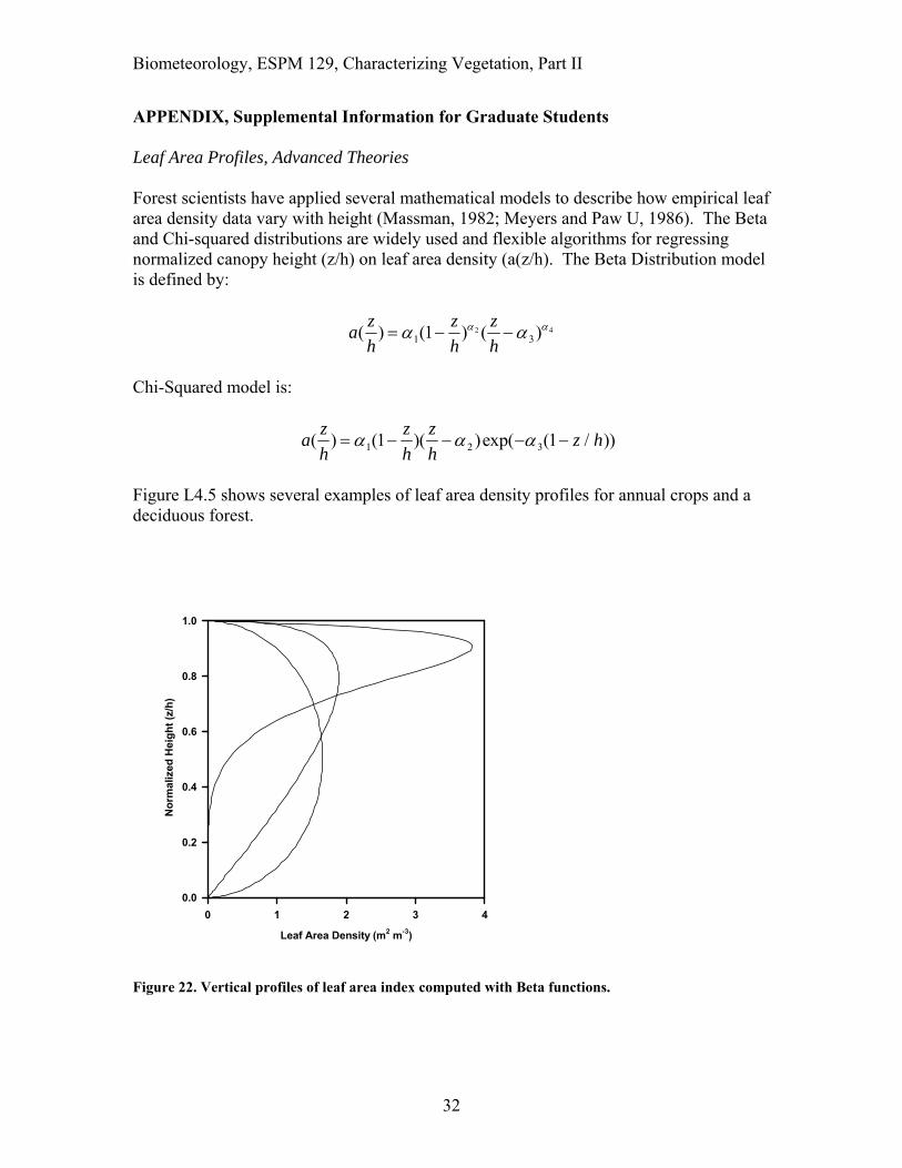
APPENDIX, Supplemental Information for Graduate Students Leaf Area Profiles, Advanced Theories Forest scientists have applied several mathematical models to describe how empirical leaf area density data vary with height (Massman, 1982; Meyers and Paw U, 1986). The Beta and Chi-squared distributions are widely used and flexible algorithms for regressing normalized canopy height (z/h) on leaf area density (a(z/h). The Beta Distribution model is defined by:

az

h

z

h

z

h( ) ( ) ( )

1 31 2 4

Chi-Squared model is:

az

h

z

h

z

hz h( ) ( )( )exp( ( / )) 1 2 31 1

Figure L4.5 shows several examples of leaf area density profiles for annual crops and a deciduous forest.

Figure 22. Vertical profiles of leaf area index computed with Beta functions.

Leaf Area Density (m2 m-3)

0 1 2 3 4

No

rmal

ized

Hei

gh

t (z

/h)

0.0

0.2

0.4

0.6

0.8

1.0


33

In crops and plantations, the leaf area density profile is unimodal and elevated. Little leaf area is below 0.25 h. As discussed above, multi-species forest canopies possess complex profiles that vary with time. Below is an example of the diverse ability of the beta distribution to mimic the leaf area density profile for a number of vegetation types


34

Figure 23 Examples of leaf area index profiles for crops and forests. Meyers and Paw U, 1986

Leaf Inclination Angles, Advanced Theories Mathematical representation of leaf angle distributions is helpful for modeling light transmission through vegetation. Equations for computing leaf inclination angle


35

distributions can be found in work by de Wit (1965), Lemeur and Blad (1974) and Ross (1981). Leaf inclination angles distribution functions include: Leaf normal distribution function (g) (after Myneni et al., 198):

gl l l( ) ( cos )

2

1 2 (planophile)

gl l l( ) ( cos )

2

1 2 (erectophile)

gl l l( ) ( cos )

2

1 4 (plagiophile)

Alternatively: f ( ) 1 (uniform distribution)

kkk)(f

36323

2

(planophile)

kkk)(f

3121223

2

(extremophile)

k equals 90 when is in degrees

3

23

k)(f

(erectophile)

Campbell models for leaf angle density functions, ellipsoidal model

g( )sin

(cos sin )

2 3

2 3 2 2

<1

sin 1

( ) /1 2 1 2


36

>1

ln( )112

( ) /1 2 1 2

lecture 3 characterizing vegetation part 3 plants … 3 characterizing the vegetation, part ii: ......

Documents