lecture 3 inference for a single proportion: test of significance for a single proportion chi-square...
TRANSCRIPT

Lecture 3
• Inference for a Single Proportion:test of significance for a single proportionChi-square test of goodness-of –fitCh-square test for independence

Recall: Population Proportion
• Let p be the proportion of “successes” in a population. A random sample of size n is selected, and X is the count of successes in the sample.
• Suppose n is small relative to the population size, so that X can be regarded as a binomial random variable with
and (1 )np np p

Recall: Population Proportion
• We use the sample proportion as an estimator of the population proportion p. • is an unbiased estimator of p, with mean and SD:
• When n is large, is approximately normal. Thus
is approximately standard normal.
nXp /ˆ
(1 ) and
p pp
n
p̂
npp
ppz
/)1(
ˆ
p̂
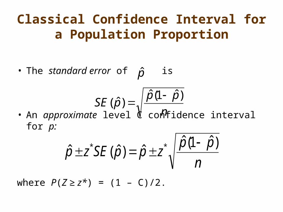
Classical Confidence Interval for a Population Proportion
• The standard error of is
• An approximate level C confidence interval for p:
where P(Z ≥ z*) = (1 – C)/2.
n
pppSE
)ˆ1(ˆ)ˆ(
n
ppzppSEzp
)ˆ1(ˆˆ)ˆ(ˆ **
p̂

Example:
A news program constructs a call-in poll about a proposed city ban on handguns. 2372 people call in to the show. Of these, 1921 oppose the ban.
Construct a 95% confidence interval for the sample proportion of people who oppose the ban.
What are the possible problems with the study design?

Solution:
• Note: Since p is a proportion, if you ever get an upper value of > 1 or lower <0, replace by 1 and 0 (respectively).

SAS
• data fraction;• input ban $ count;• cards;• yes 451• no 1921• ;• run; • proc freq order=freq;• weight count;• tables ban/ binomial alpha=0.01;• run;

• The FREQ Procedure
• Cumulative Cumulative• ban Frequency Percent Frequency Percent• • no 1921 80.99 1921 80.99• yes 451 19.01 2372 100.00
• Binomial Proportion for ban = no• • Proportion 0.8099• ASE 0.0081• 99% Lower Conf Limit 0.7891• 99% Upper Conf Limit 0.8306
• Exact Conf Limits• 99% Lower Conf Limit 0.7883• 99% Upper Conf Limit 0.8302

Testing for a single population proportion
• When n is large, is approximately normal, so
is approximately standard normal.
We may test H0: p = p0 against one of these:
– Ha: p > p0
– Ha: p < p0
– Ha: p ≠ p0
p̂
npp
ppz
/)1(
ˆ

Large-sample Significance Test for a Population Proportion
• The null hypothesis – H0: p = p0
• The test statistic is
npp
ppz
/)1(
ˆ
00
0
Alternative Hypothesis
P-value
Ha: p > p0 P(Z ≥ z)
Ha: p < p0 P(Z ≤ z)
Ha: p ≠ p0 2P(Z ≥ | z |)

Large-sample Significance Test for a Population Proportion
• How big does the sample size need to be?• The general rule of thumb to use here, as before for
approximation of binomial distribution by normal distribution, is
0 010, (1 ) 10np n p

Example:
• A claim is made that only 34% of all college students have part-time jobs. You are a little skeptical of this result and decide to conduct an experiment to show that more students work. You get a sample of 100 college students and find that 47 of these students have part-time jobs.
• Conduct a hypothesis test with = 0.05 to determine whether more than 34% of college students have part-time jobs.

Solution

SAS
• data work;• input work $ count;• cards;• yes 47• no 53• ;• run; • proc freq;• weight count;• tables work/ binomial (p=0.34 level='yes');• run;
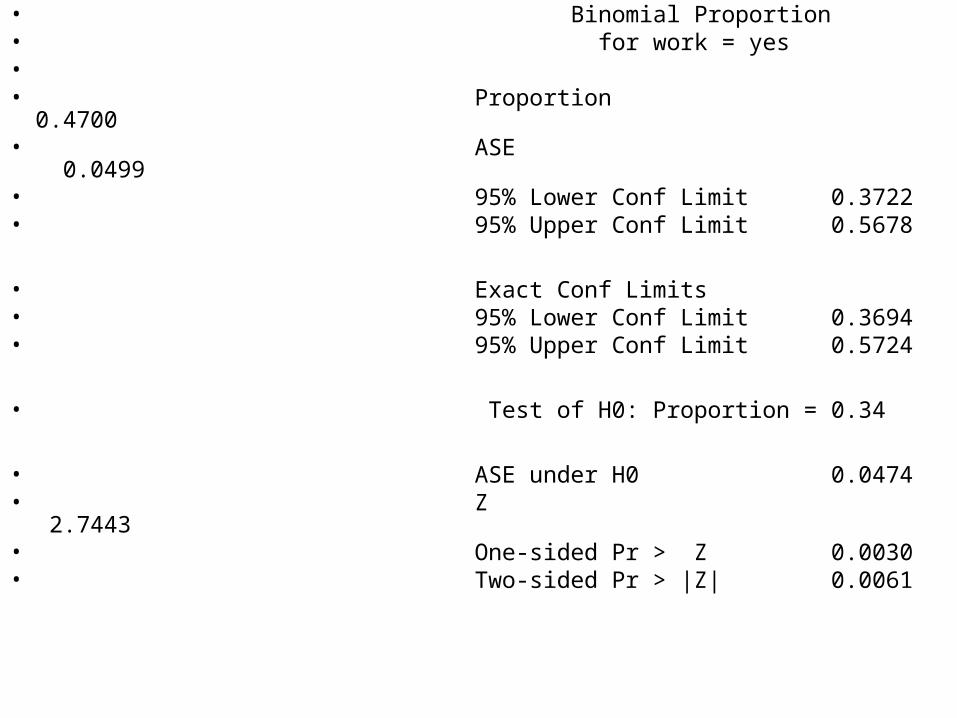
• Binomial Proportion• for work = yes• • Proportion 0.4700• ASE 0.0499• 95% Lower Conf Limit 0.3722• 95% Upper Conf Limit 0.5678
• Exact Conf Limits• 95% Lower Conf Limit 0.3694• 95% Upper Conf Limit 0.5724
• Test of H0: Proportion = 0.34
• ASE under H0 0.0474• Z 2.7443• One-sided Pr > Z 0.0030• Two-sided Pr > |Z| 0.0061

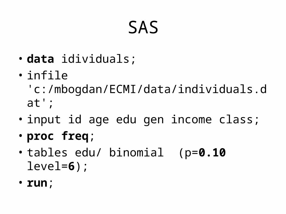
• Does proportion of people with higher education (Master or above) in American population exceeds 10 % ?
• We will use the data set individuals.dat
SAS
• data idividuals;
• infile 'c:/mbogdan/ECMI/data/individuals.dat';
• input id age edu gen income class;
• proc freq;
• tables edu/ binomial (p=0.10 level=6);
• run;

• Binomial Proportion for edu = 6• • Proportion 0.1002• ASE 0.0013• 95% Lower Conf Limit 0.0977• 95% Upper Conf Limit 0.1027
• Exact Conf Limits• 95% Lower Conf Limit 0.0977• 95% Upper Conf Limit 0.1027
• Test of H0: Proportion = 0.1
• ASE under H0 0.0013• Z 0.1565• One-sided Pr > Z 0.4378• Two-sided Pr > |Z| 0.8756

Chi-square test for goodness of fit
• categorical data; a random sample of size n• have hypothesised values for the population
proportions for each category; • these are specified in or implied by the problem• an approximate test which works when sample
size is large

Simplest case: two categories
• Example: • There are two homozygous lines of Drosophila, one with
red eyes, and one with purple eyes. It has been suggested that there is a single gene responsible for this phenotype, with the red eye trait dominant over the purple eye trait. If that is true we expect a cross of these two lines to produce F2 progeny in the ratio 3 red : 1 purple. We want to test the hypothesis that red is (autosomal) dominant. To do this we perform the cross of red-eyed and purple-eyed flies with several parents from the two lines and obtain 43 flies in the F2 generation, with 29 red-eyed flies and 14 purple-eyed flies.

Categories:
• Red eyes; hypothesised proportion = 3/(3+1) = 0.75
• "expected" number: E1 = (43)(0.75) = 32.25
• Purple eyes; hypothesised proportion 1 – = 1/(3+1) = 0.25
• "expected" number: E2 = (43)(0.25) = 10.75
• Is the red-eye trait dominant over purple?
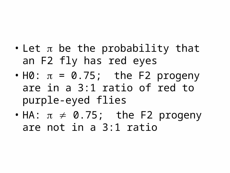
• Let be the probability that an F2 fly has red eyes
• H0: = 0.75; the F2 progeny are in a 3:1 ratio of red to purple-eyed flies
• HA: 0.75; the F2 progeny are not in a 3:1 ratio

Chi-square goodness of fit test
2 = (observed - expected)2 / expected = (O-E)2/E
• Under HO 2 has a chi-square distribution with df = #categories - 1 = 1.
• Test at level = 0.05 ; Critical value = 3.84

Chi-square distributions with df=2 and 4:

• P-value for chi-square test is:• This is always the right tail of the distribution.
2 2( )P X


Solution
SAS
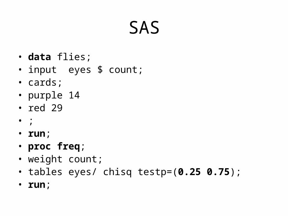
• data flies;• input eyes $ count;• cards;• purple 14• red 29• ;• run; • proc freq;• weight count;• tables eyes/ chisq testp=(0.25 0.75);• run;

• Cumulative Cumulativeeyes Frequency Percent Percent Frequency
Percent• • purple 14 32.56 25.00 14 32.56• red 29 67.44 75.00 43 100.00
• Chi-Square Test• for Specified Proportions• • Chi-Square 1.3101• DF 1• Pr > ChiSq 0.2524

• proc freq;
• weight count;
• tables eyes/ binomial (p=0.25);
• run;
• Test of H0: Proportion = 0.25
• ASE under H0 0.0660
• Z 1.1446
• One-sided Pr > Z 0.1262
• Two-sided Pr > |Z| 0.2524
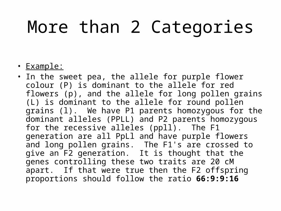
More than 2 Categories
• Example:• In the sweet pea, the allele for purple flower colour (P) is
dominant to the allele for red flowers (p), and the allele for long pollen grains (L) is dominant to the allele for round pollen grains (l). We have P1 parents homozygous for the dominant alleles (PPLL) and P2 parents homozygous for the recessive alleles (ppll). The F1 generation are all PpLl and have purple flowers and long pollen grains. The F1's are crossed to give an F2 generation. It is thought that the genes controlling these two traits are 20 cM apart. If that were true then the F2 offspring proportions should follow the ratio 66:9:9:16

• 66% purple/long : PPLL or PpLL or PPLl or PpLl,
• 9% purple/round : PPll or Ppll,
• 9% red/long = ppLL or ppLl,
• 16% red/round = ppll
• 381 F2 offspring are collected, and we observe
• 284 purple/long
• 21 purple/round
• 21 red/long
• 55 red/round
• Are these genes 20 cM apart?
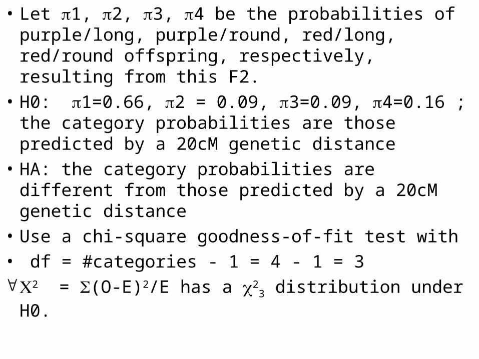
• Let 1, 2, 3, 4 be the probabilities of purple/long, purple/round, red/long, red/round offspring, respectively, resulting from this F2.
• H0: 1=0.66, 2 = 0.09, 3=0.09, 4=0.16 ; the category probabilities are those predicted by a 20cM genetic distance
• HA: the category probabilities are different from those predicted by a 20cM genetic distance
• Use a chi-square goodness-of-fit test with
• df = #categories - 1 = 4 - 1 = 32 = (O-E)2/E has a 2
3 distribution under H0.

Solution
• Test at level = 0.05; critical value for 23
is 7.81. Will reject H0 if 2 > 7.81

• data peas;• input colour $ shape $ count;• cards;• purple long 284• purple round 21• red long 21• red round 55• ;• run;
• data peas; set peas;• if ((colour eq 'purple')*(shape eq 'long')) then cs='pl';• if ((colour eq 'purple')*(shape eq 'round')) then cs='pr';• if ((colour eq 'red')*(shape eq 'long')) then cs='rl';• if ((colour eq 'red')*(shape eq 'round')) then cs='rr';• run;
• proc freq data=peas;• weight count;• tables cs/ chisq testp=(0.66 0.09 0.09 0.16);• run;

• The FREQ Procedure
• Test Cumulative Cumulative• cs Frequency Percent Percent Frequency Percent• • pl 284 74.54 66.00 284 74.54• pr 21 5.51 9.00 305 80.05• rl 21 5.51 9.00 326 85.56• rr 55 14.44 16.00 381 100.00
• Chi-Square Test• for Specified Proportions• • Chi-Square 15.0953• DF 3• Pr > ChiSq 0.0017

Test of independenceExample:
• Do men and women participate in sport for the same reasons?• 67 males and 67 females examined. Results:
• HSC-HM female 14• HSC-HM male 31• HSC-LM female 7• HSC-LM male 18• LSC-HM female 21• LSC-HM male 5• LSC-LM female 25• LSC-LM male 13
Legend: HSC (LSC)-high (low) social comparison; HM (LM)-high (low) mastery

Table of goal by sex goal sex Frequency‚ ‚ Percent ‚ ‚ ‚female ‚male ‚ Total ƒƒƒƒƒƒƒƒƒˆƒƒƒƒƒƒƒƒˆƒƒƒƒƒƒƒƒˆ HSC-HM ‚ 14 ‚ 31 ‚ ‚ ‚ ‚ ‚ 10.45 ‚ ‚ ‚ ‚ ‚ ‚ ‚ ‚ ƒƒƒƒƒƒƒƒƒˆƒƒƒƒƒƒƒƒˆƒƒƒƒƒƒƒƒˆ HSC-LM ‚ 7 ‚ 18 ‚ ‚ ‚ ‚ ‚ ‚ ‚ ‚ ‚ ‚ ‚ ‚ ‚ ƒƒƒƒƒƒƒƒƒˆƒƒƒƒƒƒƒƒˆƒƒƒƒƒƒƒƒˆ LSC-HM ‚ 21 ‚ 5 ‚ ‚ ‚ ‚ ‚ ‚ ‚ ‚ ‚ ‚ ‚ ‚ ‚ ƒƒƒƒƒƒƒƒƒˆƒƒƒƒƒƒƒƒˆƒƒƒƒƒƒƒƒˆ LSC-LM ‚ 25 ‚ 13 ‚ ‚ ‚ ‚ ‚ ‚ ‚ ‚ ‚ ‚ ‚ ‚ ‚ ƒƒƒƒƒƒƒƒƒˆƒƒƒƒƒƒƒƒˆƒƒƒƒƒƒƒƒˆ Total 134
Complete “Percent”—i.e. give the JOINT distribution of “goal” and “sex”. “goal”-column variable (often response), “sex”-row variable (often explanatory)

goal sex Frequency‚ Expected ‚ Percent ‚ Row Pct ‚ Col Pct ‚female ‚male ‚ Total ƒƒƒƒƒƒƒƒƒˆƒƒƒƒƒƒƒƒˆƒƒƒƒƒƒƒƒˆ HSC-HM ‚ 14 ‚ 31 ‚ 45 ‚ ‚ ‚ ‚ 10.45 ‚ 23.13 ‚ 33.58 ‚ ‚ ‚ ‚ ‚ ‚ ƒƒƒƒƒƒƒƒƒˆƒƒƒƒƒƒƒƒˆƒƒƒƒƒƒƒƒˆ HSC-LM ‚ 7 ‚ 18 ‚ ‚ ‚ ‚ ‚ 5.22 ‚ 13.43 ‚ ‚ ‚ ‚ ‚ ‚ ‚ ƒƒƒƒƒƒƒƒƒˆƒƒƒƒƒƒƒƒˆƒƒƒƒƒƒƒƒˆ LSC-HM ‚ 21 ‚ 5 ‚ ‚ ‚ ‚ ‚ 15.67 ‚ 3.73 ‚ ‚ ‚ ‚ ‚ ‚ ‚ ƒƒƒƒƒƒƒƒƒˆƒƒƒƒƒƒƒƒˆƒƒƒƒƒƒƒƒˆ LSC-LM ‚ 25 ‚ 13 ‚ ‚ ‚ ‚ ‚ 18.66 ‚ 9.70 ‚ ‚ ‚ ‚ ‚ ‚ ‚ ƒƒƒƒƒƒƒƒƒˆƒƒƒƒƒƒƒƒˆƒƒƒƒƒƒƒƒˆ Total 134 100.00
Find the MARGINAL distribution of goal. Find the MARGINAL distribution of sex.

MARGINAL distribution of goal in this study The FREQ Procedure Cumulative Cumulative goal Frequency Percent Frequency Percent ƒƒƒƒƒƒƒƒƒƒƒƒƒƒƒƒƒƒƒƒƒƒƒƒƒƒƒƒƒƒƒƒƒƒƒƒƒƒƒƒƒƒƒƒƒƒƒƒƒƒƒƒƒƒƒƒƒƒƒ HSC-HM 45 33.58 45 33.58 HSC-LM 25 18.66 70 52.24 LSC-HM 26 19.40 96 71.64 LSC-LM 38 28.36 134 100.00 Percentage ‚ ***** ‚ ***** ‚ ***** ‚ ***** 30 ˆ ***** ‚ ***** ‚ ***** ***** ‚ ***** ***** ‚ ***** ***** 25 ˆ ***** ***** ‚ ***** ***** ‚ ***** ***** ‚ ***** ***** ‚ ***** ***** 20 ˆ ***** ***** ‚ ***** ***** ***** ***** ‚ ***** ***** ***** ***** ‚ ***** ***** ***** ***** ‚ ***** ***** ***** ***** 15 ˆ ***** ***** ***** ***** ‚ ***** ***** ***** ***** ‚ ***** ***** ***** ***** ‚ ***** ***** ***** ***** ‚ ***** ***** ***** ***** 10 ˆ ***** ***** ***** ***** ‚ ***** ***** ***** ***** ‚ ***** ***** ***** ***** ‚ ***** ***** ***** ***** ‚ ***** ***** ***** ***** 5 ˆ ***** ***** ***** ***** ‚ ***** ***** ***** ***** ‚ ***** ***** ***** ***** ‚ ***** ***** ***** ***** ‚ ***** ***** ***** ***** Šƒƒƒƒƒƒƒƒƒƒƒƒƒƒƒƒƒƒƒƒƒƒƒƒƒƒƒƒƒƒƒƒƒƒƒƒƒƒƒƒƒƒƒƒƒƒƒƒƒƒƒƒƒƒƒ HSC-HM HSC-LM LSC-HM LSC-LM

MARGINAL distribution of sex in this study. Cumulative Cumulative sex Frequency Percent Frequency Percent ƒƒƒƒƒƒƒƒƒƒƒƒƒƒƒƒƒƒƒƒƒƒƒƒƒƒƒƒƒƒƒƒƒƒƒƒƒƒƒƒƒƒƒƒƒƒƒƒƒƒƒƒƒƒƒƒƒƒƒ female 67 50.00 67 50.00 male 67 50.00 134 100.00 Percentage 50 ˆ ***** ***** ‚ ***** ***** ‚ ***** ***** ‚ ***** ***** ‚ ***** ***** 40 ˆ ***** ***** ‚ ***** ***** ‚ ***** ***** ‚ ***** ***** ‚ ***** ***** 30 ˆ ***** ***** ‚ ***** ***** ‚ ***** ***** ‚ ***** ***** ‚ ***** ***** 20 ˆ ***** ***** ‚ ***** ***** ‚ ***** ***** ‚ ***** ***** ‚ ***** ***** 10 ˆ ***** ***** ‚ ***** ***** ‚ ***** ***** ‚ ***** ***** ‚ ***** ***** Šƒƒƒƒƒƒƒƒƒƒƒƒƒƒƒƒƒƒƒƒƒƒƒƒƒƒƒƒƒƒƒ female male sex
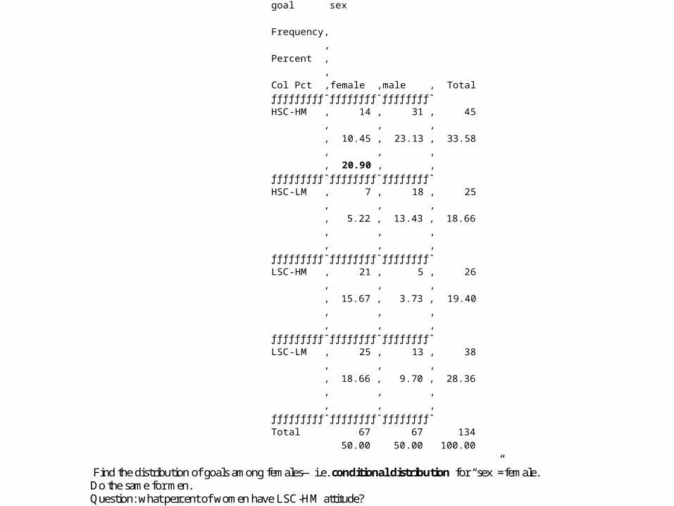
goal sex Frequency‚ ‚ Percent ‚ ‚ Col Pct ‚female ‚male ‚ Total ƒƒƒƒƒƒƒƒƒˆƒƒƒƒƒƒƒƒˆƒƒƒƒƒƒƒƒˆ HSC-HM ‚ 14 ‚ 31 ‚ 45 ‚ ‚ ‚ ‚ 10.45 ‚ 23.13 ‚ 33.58 ‚ ‚ ‚ ‚ 20.90 ‚ ‚ ƒƒƒƒƒƒƒƒƒˆƒƒƒƒƒƒƒƒˆƒƒƒƒƒƒƒƒˆ HSC-LM ‚ 7 ‚ 18 ‚ 25 ‚ ‚ ‚ ‚ 5.22 ‚ 13.43 ‚ 18.66 ‚ ‚ ‚ ‚ ‚ ‚ ƒƒƒƒƒƒƒƒƒˆƒƒƒƒƒƒƒƒˆƒƒƒƒƒƒƒƒˆ LSC-HM ‚ 21 ‚ 5 ‚ 26 ‚ ‚ ‚ ‚ 15.67 ‚ 3.73 ‚ 19.40 ‚ ‚ ‚ ‚ ‚ ‚ ƒƒƒƒƒƒƒƒƒˆƒƒƒƒƒƒƒƒˆƒƒƒƒƒƒƒƒˆ LSC-LM ‚ 25 ‚ 13 ‚ 38 ‚ ‚ ‚ ‚ 18.66 ‚ 9.70 ‚ 28.36 ‚ ‚ ‚ ‚ ‚ ‚ ƒƒƒƒƒƒƒƒƒˆƒƒƒƒƒƒƒƒˆƒƒƒƒƒƒƒƒˆ Total 67 67 134 50.00 50.00 100.00
Find the distribution of goals among females—i.e. conditional distribution for “sex”=female. Do the same for men. Question: what percent of women have LSC-HM attitude?
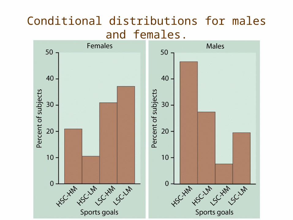
Conditional distributions for males and females.

The final result: goal sex Frequency‚ ‚ Percent ‚ Row Pct ‚ Col Pct ‚female ‚male ‚ Total ƒƒƒƒƒƒƒƒƒˆƒƒƒƒƒƒƒƒˆƒƒƒƒƒƒƒƒˆ HSC-HM ‚ 14 ‚ 31 ‚ 45 ‚ ‚ ‚ ‚ 10.45 ‚ 23.13 ‚ 33.58 ‚ 31.11 ‚ 68.89 ‚ ‚ 20.90 ‚ 46.27 ‚ ƒƒƒƒƒƒƒƒƒˆƒƒƒƒƒƒƒƒˆƒƒƒƒƒƒƒƒˆ HSC-LM ‚ 7 ‚ 18 ‚ 25 ‚ ‚ ‚ ‚ 5.22 ‚ 13.43 ‚ 18.66 ‚ 28.00 ‚ 72.00 ‚ ‚ 10.45 ‚ 26.87 ‚ ƒƒƒƒƒƒƒƒƒˆƒƒƒƒƒƒƒƒˆƒƒƒƒƒƒƒƒˆ LSC-HM ‚ 21 ‚ 5 ‚ 26 ‚ ‚ ‚ ‚ 15.67 ‚ 3.73 ‚ 19.40 ‚ 80.77 ‚ 19.23 ‚ ‚ 31.34 ‚ 7.46 ‚ ƒƒƒƒƒƒƒƒƒˆƒƒƒƒƒƒƒƒˆƒƒƒƒƒƒƒƒˆ LSC-LM ‚ 25 ‚ 13 ‚ 38 ‚ ‚ ‚ ‚ 18.66 ‚ 9.70 ‚ 28.36 ‚ 65.79 ‚ 34.21 ‚ ‚ 37.31 ‚ 19.40 ‚ ƒƒƒƒƒƒƒƒƒˆƒƒƒƒƒƒƒƒˆƒƒƒƒƒƒƒƒˆ Total 67 67 134 50.00 50.00 100.00
TWO-WAY table with marginal and conditional distributions.
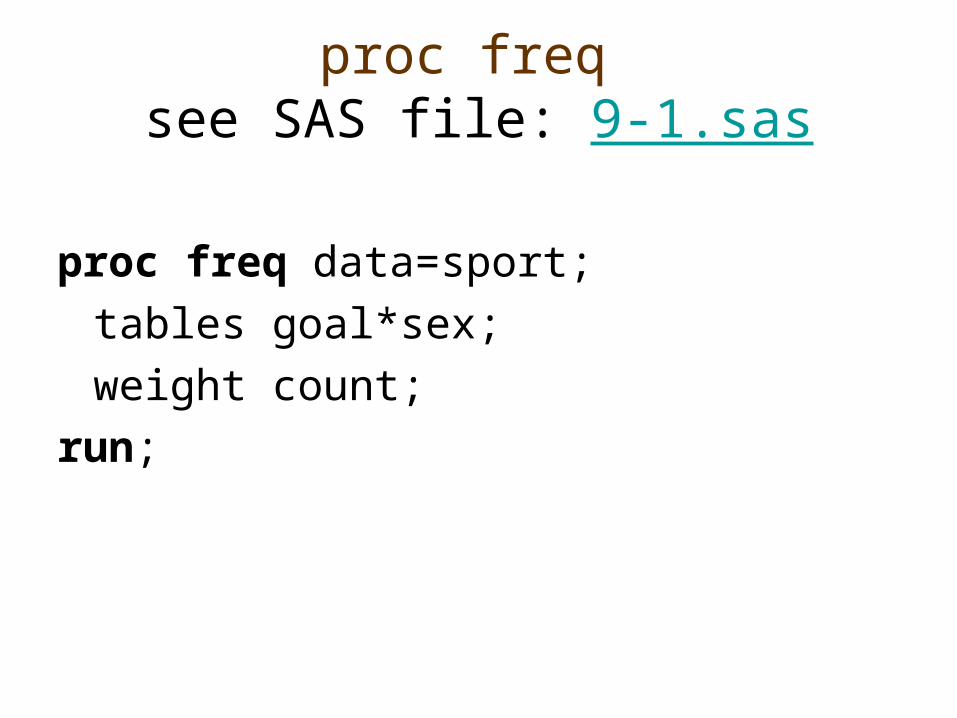
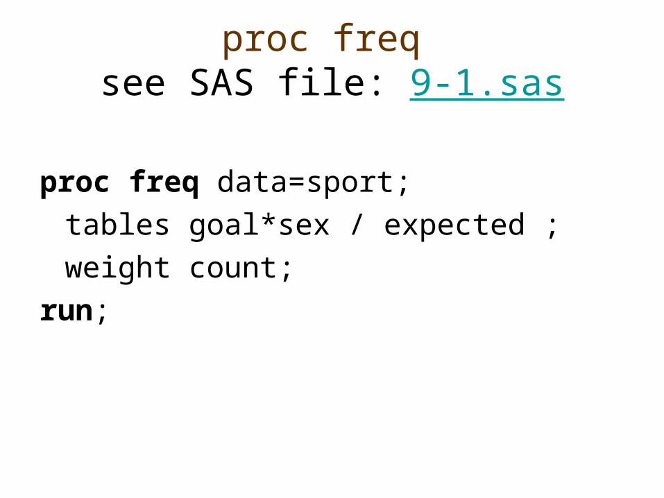
proc freq see SAS file: 9-1.sas
proc freq data=sport;
tables goal*sex;
weight count;
run;

Simpsons’s paradox:
• An association or comparison that holds for all of several groups can reverse direction when the data are combined to form a single group.
• This can be due to a lurking variable.
Example :
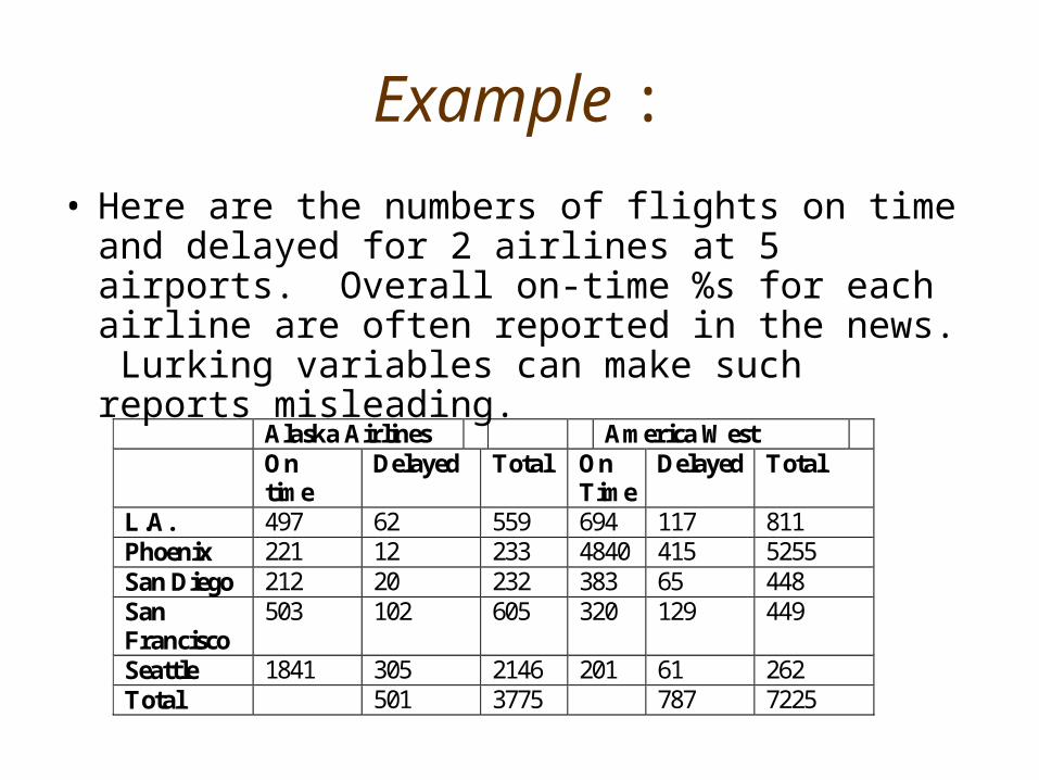
• Here are the numbers of flights on time and delayed for 2 airlines at 5 airports. Overall on-time %s for each airline are often reported in the news. Lurking variables can make such reports misleading.
Alaska Airlines America West On
time Delayed Total On
Time Delayed Total
L.A. 497 62 559 694 117 811 Phoenix 221 12 233 4840 415 5255 San Diego 212 20 232 383 65 448 San Francisco
503 102 605 320 129 449
Seattle 1841 305 2146 201 61 262 Total 501 3775 787 7225

a) Find the % of delayed flights for Alaska Airlines at each of the 5 airports, and then do the same for America West. (Note: these are not joint probabilities.)
Alaska Airlines America West L.A.
Phoenix
San Diego
San Francisco
Seattle
b) What % of all Alaska Airlines flights were delayed? What % of all America West flights were delayed? These
are the numbers usually reported.
c) America West does worse at every one of the 5 airports, yet does better overall. That sounds impossible. Explain carefully, referring to the data, how this can happen.

Perils of aggregation
• This example was essentially a Three-Way Table with variables: airline, timing, airport.
• Such tables are often reported as several two-way tables. Think a book, rather than a page.
• Adding entries from such elementary tables (“pages”) to get the overall summary (for the “book”) is aggregation and leads to ignoring the third variable (here: airport).
• This may lead to false general conclusions.

Inference for Two-Way tables
Hypothesis testing with 2-way tables• H0: there is no association between the row and
column variables (they are independent)• Ha: there is an association between the row and
column variables
• To test the hypotheses, compare observed cell counts with expected cell counts.
• Expected=calculated under the assumption that the null hypothesis is true.

expected count =
Here n = total # of observations for the table.
row total column total
n

goal sex Frequency‚ Expected ‚ Percent ‚ Row Pct ‚ Col Pct ‚female ‚male ‚ Total ƒƒƒƒƒƒƒƒƒˆƒƒƒƒƒƒƒƒˆƒƒƒƒƒƒƒƒˆ HSC-HM ‚ 14 ‚ 31 ‚ 45 ‚ 22.5 ‚ ‚ ‚ 10.45 ‚ 23.13 ‚ 33.58 ‚ 31.11 ‚ 68.89 ‚ ‚ 20.90 ‚ 46.27 ‚ ƒƒƒƒƒƒƒƒƒˆƒƒƒƒƒƒƒƒˆƒƒƒƒƒƒƒƒˆ HSC-LM ‚ 7 ‚ 18 ‚ 25 ‚ ‚ ‚ ‚ 5.22 ‚ 13.43 ‚ 18.66 ‚ 28.00 ‚ 72.00 ‚ ‚ 10.45 ‚ 26.87 ‚ ƒƒƒƒƒƒƒƒƒˆƒƒƒƒƒƒƒƒˆƒƒƒƒƒƒƒƒˆ LSC-HM ‚ 21 ‚ 5 ‚ 26 ‚ ‚ ‚ ‚ 15.67 ‚ 3.73 ‚ 19.40 ‚ 80.77 ‚ 19.23 ‚ ‚ 31.34 ‚ 7.46 ‚ ƒƒƒƒƒƒƒƒƒˆƒƒƒƒƒƒƒƒˆƒƒƒƒƒƒƒƒˆ LSC-LM ‚ 25 ‚ 13 ‚ 38 ‚ ‚ ‚ ‚ 18.66 ‚ 9.70 ‚ 28.36 ‚ 65.79 ‚ 34.21 ‚ ‚ 37.31 ‚ 19.40 ‚ ƒƒƒƒƒƒƒƒƒˆƒƒƒƒƒƒƒƒˆƒƒƒƒƒƒƒƒˆ Total 67 67 134 50.00 50.00 100.00
Calculate EXPECTED counts.
proc freq see SAS file: 9-1.sas
proc freq data=sport;
tables goal*sex / expected ;
weight count;
run;

Test statistic: Chi Square Test Statistic
2
2 observed count - expected count
expected countX

distribution
• The X2 test statistic has an approximately chi-square distribution.
• To use the chi-square table, you need the degrees of freedom:
(r-1)(c-1)=(#rows-1)(#colums-1).
• Our example has (4-1)(2-1)=3 df.
2

Finale: Do men and women participate in
sport for the same reasons? Frequency‚ Expected ‚ Percent ‚ Row Pct ‚ Col Pct ‚female ‚male ‚ Total ƒƒƒƒƒƒƒƒƒˆƒƒƒƒƒƒƒƒˆƒƒƒƒƒƒƒƒˆ HSC-HM ‚ 14 ‚ 31 ‚ 45 ‚ 22.5 ‚ 22.5 ‚ ‚ 10.45 ‚ 23.13 ‚ 33.58 ‚ 31.11 ‚ 68.89 ‚ ‚ 20.90 ‚ 46.27 ‚ ƒƒƒƒƒƒƒƒƒˆƒƒƒƒƒƒƒƒˆƒƒƒƒƒƒƒƒˆ HSC-LM ‚ 7 ‚ 18 ‚ 25 ‚ 12.5 ‚ 12.5 ‚ ‚ 5.22 ‚ 13.43 ‚ 18.66 ‚ 28.00 ‚ 72.00 ‚ ‚ 10.45 ‚ 26.87 ‚ ƒƒƒƒƒƒƒƒƒˆƒƒƒƒƒƒƒƒˆƒƒƒƒƒƒƒƒˆ LSC-HM ‚ 21 ‚ 5 ‚ 26 ‚ 13 ‚ 13 ‚ ‚ 15.67 ‚ 3.73 ‚ 19.40 ‚ 80.77 ‚ 19.23 ‚ ‚ 31.34 ‚ 7.46 ‚ ƒƒƒƒƒƒƒƒƒˆƒƒƒƒƒƒƒƒˆƒƒƒƒƒƒƒƒˆ LSC-LM ‚ 25 ‚ 13 ‚ 38 ‚ 19 ‚ 19 ‚ ‚ 18.66 ‚ 9.70 ‚ 28.36 ‚ 65.79 ‚ 34.21 ‚ ‚ 37.31 ‚ 19.40 ‚ ƒƒƒƒƒƒƒƒƒˆƒƒƒƒƒƒƒƒˆƒƒƒƒƒƒƒƒˆ Total 67 67 134 50.00 50.00 100.00
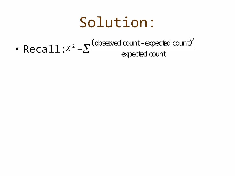
Solution:
• Recall: 2
2 observed count - expected count
expected countX

proc freq see SAS file: 9-1.sas
proc freq data=sport;
tables goal*sex / expected chisq;
weight count;
run;

The FREQ Procedure (output): Statistics for Table of goal by sex Statistic DF Value Prob ƒƒƒƒƒƒƒƒƒƒƒƒƒƒƒƒƒƒƒƒƒƒƒƒƒƒƒƒƒƒƒƒƒƒƒƒƒƒƒƒƒƒƒƒƒƒƒƒƒƒƒƒƒƒ Chi-Square 3 24.8978 <.0001 Likelihood Ratio Chi-Square 3 26.0362 <.0001 Mantel-Haenszel Chi-Square 1 16.2249 <.0001 Phi Coefficient 0.4311 Contingency Coefficient 0.3958 Cramer's V 0.4311 Sample Size = 134

Rules for using the test:
• The chi-square test becomes more accurate as the cell counts increase and for tables larger than 2x2.
• For tables larger than 2x2: use chi-square test whenever:
the average of the expected counts is 5 or more the smallest expected count is 1 or more <20% of cells have expected counts of less than 5.
• For 2x2 tables: use chi-square test whenever all 4 expected cell counts are 5 or more

Example:
• 356 volunteers classified according socioeconimic status (SES) and smoking habits.
• Is smoking associated with SES?
smoking SES Frequency‚ Percent ‚ Row Pct ‚ Col Pct ‚high ‚low ‚middle ‚ Total ƒƒƒƒƒƒƒƒƒˆƒƒƒƒƒƒƒƒˆƒƒƒƒƒƒƒƒˆƒƒƒƒƒƒƒƒˆ current ‚ 51 ‚ 43 ‚ 22 ‚ 116 ‚ 14.33 ‚ 12.08 ‚ 6.18 ‚ 32.58 ‚ 43.97 ‚ 37.07 ‚ 18.97 ‚ ‚ 24.17 ‚ 46.24 ‚ 42.31 ‚ ƒƒƒƒƒƒƒƒƒˆƒƒƒƒƒƒƒƒˆƒƒƒƒƒƒƒƒˆƒƒƒƒƒƒƒƒˆ former ‚ 92 ‚ 28 ‚ 21 ‚ 141 ‚ 25.84 ‚ 7.87 ‚ 5.90 ‚ 39.61 ‚ 65.25 ‚ 19.86 ‚ 14.89 ‚ ‚ 43.60 ‚ 30.11 ‚ 40.38 ‚ ƒƒƒƒƒƒƒƒƒˆƒƒƒƒƒƒƒƒˆƒƒƒƒƒƒƒƒˆƒƒƒƒƒƒƒƒˆ never ‚ 68 ‚ 22 ‚ 9 ‚ 99 ‚ 19.10 ‚ 6.18 ‚ 2.53 ‚ 27.81 ‚ 68.69 ‚ 22.22 ‚ 9.09 ‚ ‚ 32.23 ‚ 23.66 ‚ 17.31 ‚ ƒƒƒƒƒƒƒƒƒˆƒƒƒƒƒƒƒƒˆƒƒƒƒƒƒƒƒˆƒƒƒƒƒƒƒƒˆ Total 211 93 52 356 59.27 26.12 14.61 100.00

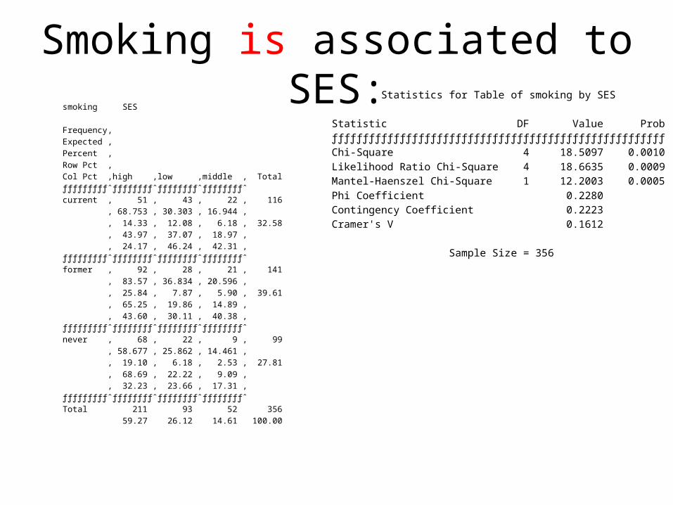
Smoking is associated to SES: smoking SES Frequency‚ Expected ‚ Percent ‚ Row Pct ‚ Col Pct ‚high ‚low ‚middle ‚ Total ƒƒƒƒƒƒƒƒƒˆƒƒƒƒƒƒƒƒˆƒƒƒƒƒƒƒƒˆƒƒƒƒƒƒƒƒˆ current ‚ 51 ‚ 43 ‚ 22 ‚ 116 ‚ 68.753 ‚ 30.303 ‚ 16.944 ‚ ‚ 14.33 ‚ 12.08 ‚ 6.18 ‚ 32.58 ‚ 43.97 ‚ 37.07 ‚ 18.97 ‚ ‚ 24.17 ‚ 46.24 ‚ 42.31 ‚ ƒƒƒƒƒƒƒƒƒˆƒƒƒƒƒƒƒƒˆƒƒƒƒƒƒƒƒˆƒƒƒƒƒƒƒƒˆ former ‚ 92 ‚ 28 ‚ 21 ‚ 141 ‚ 83.57 ‚ 36.834 ‚ 20.596 ‚ ‚ 25.84 ‚ 7.87 ‚ 5.90 ‚ 39.61 ‚ 65.25 ‚ 19.86 ‚ 14.89 ‚ ‚ 43.60 ‚ 30.11 ‚ 40.38 ‚ ƒƒƒƒƒƒƒƒƒˆƒƒƒƒƒƒƒƒˆƒƒƒƒƒƒƒƒˆƒƒƒƒƒƒƒƒˆ never ‚ 68 ‚ 22 ‚ 9 ‚ 99 ‚ 58.677 ‚ 25.862 ‚ 14.461 ‚ ‚ 19.10 ‚ 6.18 ‚ 2.53 ‚ 27.81 ‚ 68.69 ‚ 22.22 ‚ 9.09 ‚ ‚ 32.23 ‚ 23.66 ‚ 17.31 ‚ ƒƒƒƒƒƒƒƒƒˆƒƒƒƒƒƒƒƒˆƒƒƒƒƒƒƒƒˆƒƒƒƒƒƒƒƒˆ Total 211 93 52 356 59.27 26.12 14.61 100.00
Statistics for Table of smoking by SES Statistic DF Value Prob ƒƒƒƒƒƒƒƒƒƒƒƒƒƒƒƒƒƒƒƒƒƒƒƒƒƒƒƒƒƒƒƒƒƒƒƒƒƒƒƒƒƒƒƒƒƒƒƒƒƒƒƒƒƒ Chi-Square 4 18.5097 0.0010 Likelihood Ratio Chi-Square 4 18.6635 0.0009 Mantel-Haenszel Chi-Square 1 12.2003 0.0005 Phi Coefficient 0.2280 Contingency Coefficient 0.2223 Cramer's V 0.1612 Sample Size = 356

Example (Aspirin study):
• 21,996 male American physicians.
• Half of these took aspirin.
• After 3 years, 139 of those who took aspirin and 239 of those who took placebo had had heart attacks.
• Determine whether there is an association of aspirin with heart attacks.

Solution:

fate treatment Frequency‚ Expected ‚ Percent ‚ Row Pct ‚ Col Pct ‚aspirin ‚placebo ‚ Total ƒƒƒƒƒƒƒƒƒˆƒƒƒƒƒƒƒƒˆƒƒƒƒƒƒƒƒˆ heart_at ‚ 139 ‚ 239 ‚ 378 ‚ 189 ‚ 189 ‚ ‚ 0.63 ‚ 1.09 ‚ 1.72 ‚ 36.77 ‚ 63.23 ‚ ‚ 1.26 ‚ 2.17 ‚ ƒƒƒƒƒƒƒƒƒˆƒƒƒƒƒƒƒƒˆƒƒƒƒƒƒƒƒˆ no_heart ‚ 10859 ‚ 10759 ‚ 21618 ‚ 10809 ‚ 10809 ‚ ‚ 49.37 ‚ 48.91 ‚ 98.28 ‚ 50.23 ‚ 49.77 ‚ ‚ 98.74 ‚ 97.83 ‚ ƒƒƒƒƒƒƒƒƒˆƒƒƒƒƒƒƒƒˆƒƒƒƒƒƒƒƒˆ Total 10998 10998 21996 50.00 50.00 100.00

Statistics for Table of fate by treatment Statistic DF Value Prob ƒƒƒƒƒƒƒƒƒƒƒƒƒƒƒƒƒƒƒƒƒƒƒƒƒƒƒƒƒƒƒƒƒƒƒƒƒƒƒƒƒƒƒƒƒƒƒƒƒƒƒƒƒƒ Chi-Square 1 26.9176 <.0001 Likelihood Ratio Chi-Square 1 27.2352 <.0001 Continuity Adj. Chi-Square 1 26.3819 <.0001 Mantel-Haenszel Chi-Square 1 26.9164 <.0001 Phi Coefficient -0.0350 Contingency Coefficient 0.0350 Cramer's V -0.0350 Fisher's Exact Test ƒƒƒƒƒƒƒƒƒƒƒƒƒƒƒƒƒƒƒƒƒƒƒƒƒƒƒƒƒƒƒƒƒƒ Cell (1,1) Frequency (F) 139 Left-sided Pr <= F 1.203E-07 Right-sided Pr >= F 1.0000 Table Probability (P) 5.228E-08 Two-sided Pr <= P 2.407E-07 Sample Size = 21996 Conclusion: Aspirin reduces chance of heart attack (P<.0001).