1

Lecture #3���Nuclear Spin Hamiltonian

•  Topics–  Liouville-von Neuman equation–  Time-averaged versus instantaneous spin Hamiltonian–  Chemical shift and J, dipolar, and quadrupolar coupling

•  Reading assignments–  van de Ven: Chapters 2.1-2.2 –  Levitt, Chapters 7 (optional)

2

Coherences•  Nuclear spins can be thought of as weak magnetic dipoles,

each with a well defined direction of polarization.

€

2ˆ I z ˆ S z

No net tendency for I or S spins to be ±zIf I or S is ±z, increased probability paired spin is ±z

•  Summing the polarization across many spins can result in net phase coherences.

€

ˆ S z IS

Net tendency for S spins to be +zNo net tendency for I spins in any direction

3

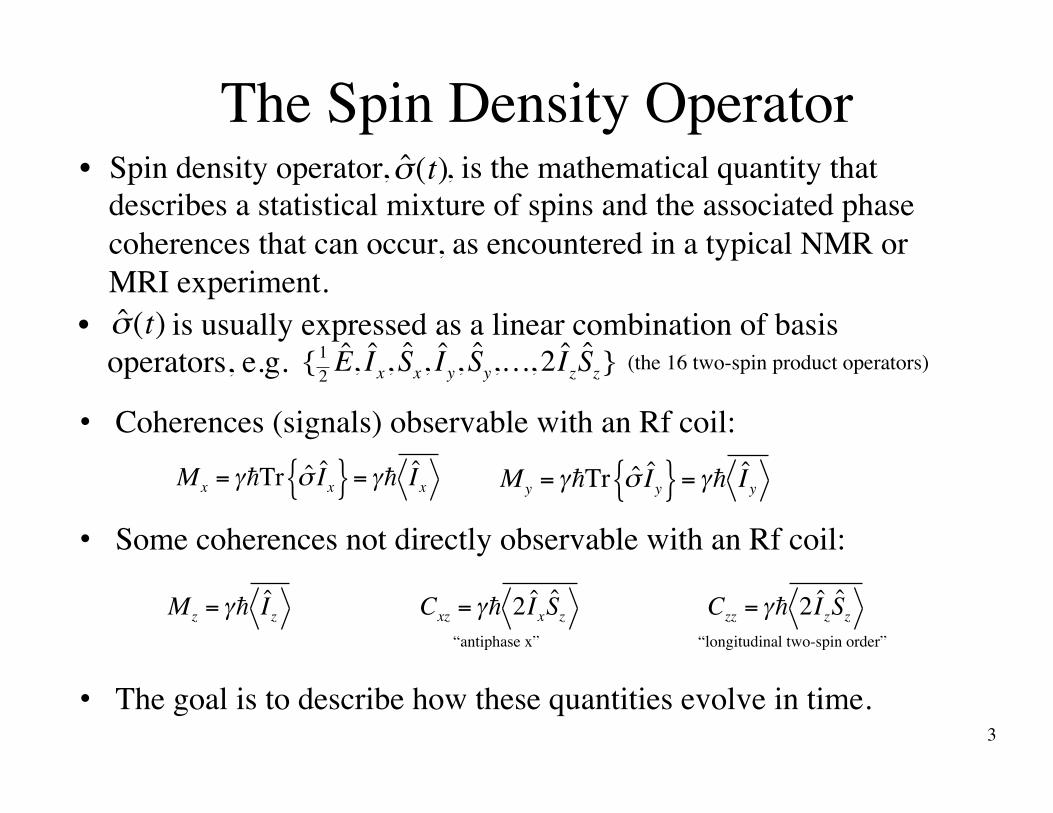
The Spin Density Operator•  Spin density operator, , is the mathematical quantity that

describes a statistical mixture of spins and the associated phase coherences that can occur, as encountered in a typical NMR or MRI experiment.

€

ˆ σ (t)

Mx = γ!Tr σ I x{ }= γ! I x

•  Coherences (signals) observable with an Rf coil:

My = γ!Tr σ I y{ }= γ! I y

Mz = γ! Iz Cxz = γ! 2 I xSz“antiphase x”

Czz = γ! 2 IzSz“longitudinal two-spin order”

•  The goal is to describe how these quantities evolve in time.

•  is usually expressed as a linear combination of basis operators, e.g.

€

ˆ σ (t)(the 16 two-spin product operators){12 E, I x, Sx, I y, Sy,…, 2 IzSz}

•  Some coherences not directly observable with an Rf coil:

4

Liouville-von Neumann Equation•  Time evolution of :

€

ˆ σ (t)

∂∂tσ = −i ˆHσ is the Hamiltonian operator

and corresponds to the energy of the system (E ).

ˆ H

/!

•  The key, yet again, is finding the Hamiltonian!

€

ˆ I z

€

ˆ I x

€

ˆ I yσ t( )σ 0( )

•  can often be expressed as sum of a large static component plus a small time-varying perturbation: , leading to…H = H0 + H1 t( )

ˆ H

∂∂tσ = −i ˆH0σ − ˆΓ σ − σ B( )

Relaxation superoperator (a function of )

Rotations Relaxation

H1

(Compare with Bloch’s equations)

5

Spin-Lattice Disconnect•  Complete QM description of a molecule involves lots of terms in

the Hamiltonian (nuclear spin, molecular motion, electron-nucleus interactions, etc).

•  Previously, we assumed a negligible interaction between the nuclear spins and the lattice:

ˆ H = ˆ H l + ˆ H s + ˆ H i

ˆ H ≈ ˆ H l + ˆ H s

lattice spin interaction term

∂∂t

ˆ σ = −i ˆ ˆ H s ˆ σ and just solved

•  Now we need to take a closer look at the interaction term, which includes effects such as spin operator coefficients that depend on molecular orientation, etc.

6

The Nuclear Spin Hamiltonian

Examples:2) interactions with dipole fields of other nuclei 3) nuclear-electron couplings

•  is the sum of different terms representing different physical interactions. H

€

ˆ H = ˆ H 1 + ˆ H 2 + ˆ H 3 +!1) interaction of spin with

€

B0

•  In general, we can think of an atomic nucleus as a lumpy magnet with a (possibly non-uniform) positive electric charge

The nuclear electric charge interacts with electric fields

The nuclear magnetic moment interacts with magnetic fields

€

ˆ H = ˆ H elec + ˆ H mag

•  The spin Hamiltonian contains terms which describe the orientation dependence of the nuclear energy

7

Electromagnetic Interactions

•  Electric interactions

Hence, for spin-½ nuclei there are no electrical energy terms that depend on orientation or internal nuclear structure, and they behaves exactly like point charges! Nuclei with spin > ½ have electrical quadrupolar moments.

•  Magnetic interactions

Nuclear electric charge distributions can be expressed as a sum of multipole components.

Symmetry properties: C(n)=0 for n>2I and odd interaction terms disappear

monopole dipole quadrapole

€

C(! r ) = C(0)(! r ) + C(1)(! r ) + C(2)(! r ) +"

€

ˆ H elec = 0 (for spin I =1/2)H elec ≠ 0 (for spin I >1/2)

€

ˆ H mag = − ˆ ! µ ⋅! B = −γ"ˆ

! I ⋅! B

magnetic moment

local magnetic field

8

Motional Averaging

•  Previously, we used averaging to simplify the Hamiltonian

•  Molecular motion

Molecular orientation depends on time and Hamiltonian terms can be written as . These terms were replaced by their time averages:

€

ˆ H int0 Θ(t)( )

€

ˆ H int0 = 1

τˆ H int

0 Θ(t)( )0

τ

∫ dt

Isotropic materials:

€

ˆ H intisotropic = 1

Nˆ H int

0 Θ( )∫ dΘnormalization

ergodicity

€

ˆ H int0 = ˆ H int

0 pΘ( )∫ dΘp(Θ)=probability

density for molecule having orientation Θ

•  We no longer want to make this approximation. Instead, the time variations will be analyzed as perturbations.

What does “secular” mean?

Secular Hamiltonian

9

Time-averaged Spin Hamiltonian

Rela

tive

mag

nitu

des

10

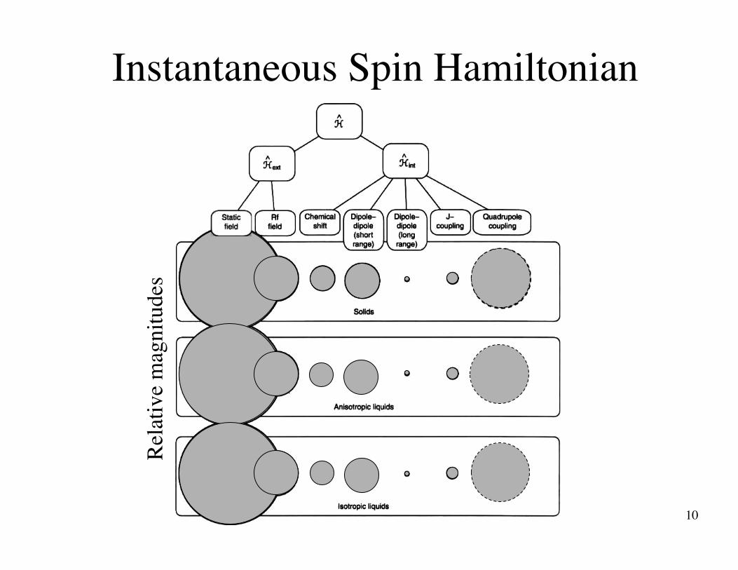
Instantaneous Spin Hamiltonian

Rela

tive

mag

nitu

des

11

Simplifications

1.  For terms in the Hamiltonian that are periodic, we use a change of basis.

•  In general, the nuclear spin Hamiltonian is quite complicated.

2.  The secular approximation

•  We’ll regularly make use of two simplifications.

ˆ !H = e−iωt ˆIz H = e−iωtIz HeiωtIzrotating frame laboratory frame

H t( ) = −ω0 Iz −ω1 I x cosωt − I y sinωt( ) Heff = − ω0 −ω( ) Iz −ω1I x

12

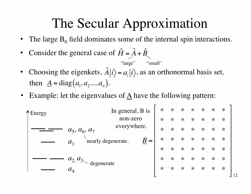
The Secular Approximation•  The large B0 field dominates some of the internal spin interactions.

•  Consider the general case of H = A+ B“large” “small”

A i = ai i•  Choosing the eigenkets, , as an orthonormal basis set,A = diag a1,a2...,an( ).then

•  Example: let the eigenvalues of A have the following pattern:

B =

* * * * * * ** * * * * * ** * * * * * ** * * * * * ** * * * * * ** * * * * * ** * * * * * *

!

"

########

$

%

&&&&&&&&

In general, B is non-zero

everywhere.

Energy

a1

a2, a3

a4

a5, a6, a7

nearly degenerate.

degenerate

13

The Secular Approximation•  The secular approximation of B is:

•  This is equivalent to omitting terms for which bmn << am − an .

Energy

a1

a2, a3

a4

a5, a6, a7

Eigenvalues of A

B0 =

* 0 0 0 0 0 00 * * 0 0 0 00 * * 0 0 0 00 0 0 * 0 0 00 0 0 0 * * *0 0 0 0 * * *0 0 0 0 * * *

!

"

########

$

%

&&&&&&&&

•  Mathematically B0 = bnn n nn∑ + bmn m n

m≠n∑

`

where the indicates summation only over terms which connect degenerate or nearly degenerate states of A.

`

•  The secular approximation for the Hamiltonian is: H ≈ A+ B0.

14

Secular Approximation Example•  Consider a spin in a large field B0 to which we add an x gradient Gx.

hence B0 = 12

γGxx 00 −γGxx

"

#$$

%

&''

•  However, è B0 >>Gxx, ΔBx, ΔBy a1 − a2 = γB0 >> γ ΔBx ± iΔBy

•  We actually can’t create the field alone (see Laplace’s Eqn)Gxx!z

•  We really have:!B = B0

!z +Gxx!z +ΔBx x, y, z( )

!x +ΔBy x, y, z( )!y

In MRI, these are often called “Maxwell” or “concomitant gradient” terms.

H = −γ!B ⋅ ˆ!I = −γB0 Iz −γGxxIz −γΔBxIx −γΔByIy = A+ BHence:

A = 12

γB0 00 −γB0

"

#$$

%

&''

B = 12

γGxx γ ΔBx + iΔBy( )γ ΔBx − iΔBy( ) −γGxx

#

$

%%%

&

'

(((

A Bwhere and

•  The secular approximation is: H = −γ!B ⋅ ˆ!I ≈ A+ B0 = −γ B0 +γGxx( ) Iz

i.e. we can safely ignore the “Maxwell” terms as is routinely done in MRI (with just a few exceptions, particularly at low field)

15

B0-Electron Interactions

•  Local effect: Chemical Shift

•  Global effects: magnetic susceptibility

When a material is placed in a magnetic field it is magnetized to some degree and this modifies the field…

€

B0s = (1− χ)B0

Hereafter we’ll use “B0” to refer to the internal field.

field inside sample bulk magnetic susceptibility applied field

Electrons in an atom circulate about B0, generating a magnetic moment opposing the applied magnetic field.

Different atoms experience different electron cloud densities.

€

B = B0(1−σ)

shielding constant(Don’t confuse with the spin density operator!)

Shielding:

16

The Zeeman Hamiltonian

€

ˆ H zeeman = −γ! ˆ I (1−σ)

! B

€

σ =σ iso = Tr(σ /3)

€

E = −γ! B ⋅! I Classical:

HZeeman = −γ (1−σ )B0 Iz

€

! µ = γ! I

€

! B •  The interaction energy between the magnetic field, , and the

magnetic moment, , is given by the Zeeman Hamiltonian.

•  The formal correction for chemical shielding is:

where

€

σ = 3× 3 shielding tensor

•  In vivo, rapid molecular tumbling averages out the non-isotropic components.

!B = [0, 0,B0 ] :•  Hence for

€

ˆ H zeeman = −γ! B ⋅! ˆ I QM:

E

€

B = 0

€

B = B0

17

Chemical Shielding Tensor•  Electron shielding is in general anisotropic, i.e. the degree of

shielding depends on the molecular orientation.•  The shielding tensor can be written as the sum of three terms:

σ =

σ xx σ xy σ xz

σ yx σ yy σ yz

σ zx σ zy σ zz

!

"

####

$

%

&&&&

=σ iso

1 0 00 1 00 0 1

!

"

###

$

%

&&&+σ 1( ) +σ 2( )

= 13 σ xx +σ yy +σ zz( )

antisymmetric

•  Both σ(1) and σ(2) are time-varying due to molecular tumbling.

•  σ(2) gives rise to a relaxation mechanism called chemical shift anisotropy (CSA). (to be discussed later in the course)

•  σ(1) causes only 2nd order effects and is typically ignored.

symmetric and traceless

See Kowalewski, pp 105-6 for details.

A little foreshadowing…

18

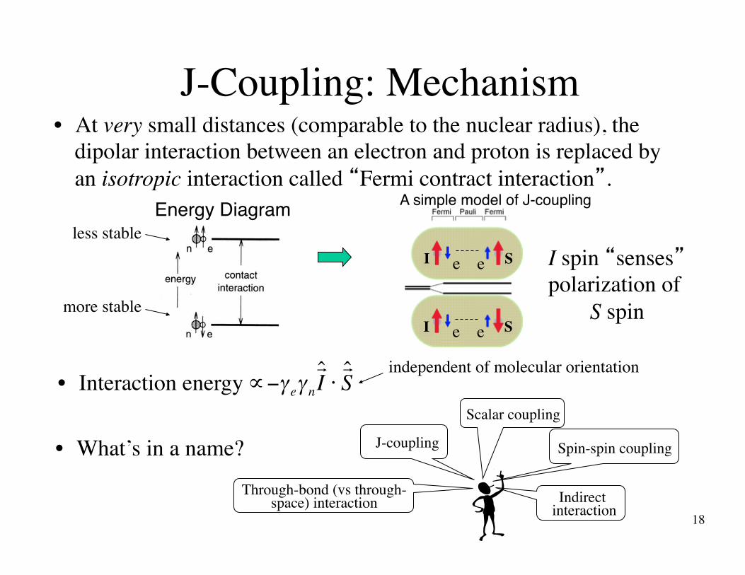
J-Coupling: Mechanism

•  What’s in a name?

•  At very small distances (comparable to the nuclear radius), the dipolar interaction between an electron and proton is replaced by an isotropic interaction called “Fermi contract interaction”.

Energy Diagramless stable

more stable

I spin “senses” polarization of

S spin

I S

I S

e e

e e

A simple model of J-coupling

€

∝−γ eγ n

! ˆ I ⋅! ˆ S •  Interaction energy

independent of molecular orientation

J-coupling

Through-bond (vs through-space) interaction

Scalar coupling

Spin-spin coupling

Indirect interaction

19

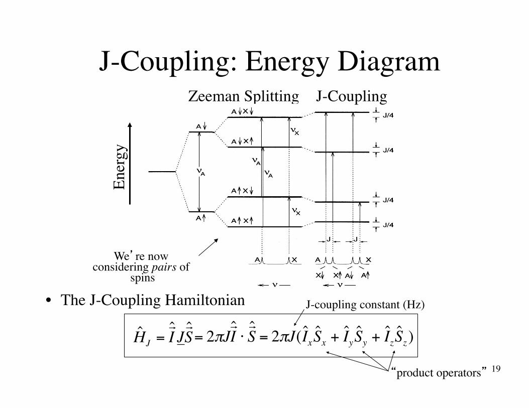
J-Coupling: Energy Diagram

€

= 2πJ! ˆ I ⋅! ˆ S

J-Coupling

€

= 2πJ( ˆ I x ˆ S x + ˆ I y ˆ S y + ˆ I z ˆ S z)

€

ˆ H J =! ˆ I J! ˆ S

Ener

gyZeeman Splitting

We’re now considering pairs of

spins

J-coupling constant (Hz)•  The J-Coupling Hamiltonian

“product operators”

20

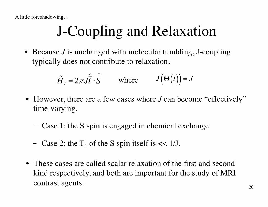
J-Coupling and Relaxation•  Because J is unchanged with molecular tumbling, J-coupling

typically does not contribute to relaxation.

A little foreshadowing…

•  However, there are a few cases where J can become “effectively” time-varying.

-  Case 1: the S spin is engaged in chemical exchange

-  Case 2: the T1 of the S spin itself is << 1/J.

•  These cases are called scalar relaxation of the first and second kind respectively, and both are important for the study of MRI contrast agents.

HJ = 2π J!I ⋅!S J Θ t( )( ) = Jwhere

21

Magnetic Dipoles•  Nuclei with spin ≠ 0 act like tiny magnetic dipoles.

permeability of free space

falls off as r3

Dipole at origin

€

Bµx =µ04π#

$ %

&

' (

µr3#

$ %

&

' ( 3sinθ cosθ( )

€

Bµy = 0

€

Bµz =µ04π#

$ %

&

' (

µr3#

$ %

&

' ( 3cos2θ −1( )

Magnetic Field in y=0 plane

Lines of Force Bµz Bµx

22

Dipolar Coupling•  Dipole fields from nearby spins interact (i.e. are coupled).

•  Rapid fall off with distance causes this to be primarily a intramolecular effect.

Water molecule

in a magnetic

field

with tumbling

Interaction is time variant!

Spins remain aligned with B0

23

The Nuclear Dipolar Coupling Hamiltonian

•  Mathematically speaking, the general expression is:

Hdipole = −µ0γ IγS4πr3

!"I ⋅!S − 3

r2(!I ⋅ !r )(

!S ⋅ !r )

#

$%

&

'( where vector from

spin I to spin S

€

! r

• Secular approximation:

€

ˆ H dipole = d 3ˆ I z ˆ S z −! ˆ I ⋅! ˆ S $

% & '

( ) where d = −

µ0γ Iγ S

4πr3 " 3cos2ΘIS −1( )dipole coupling

constantangle between B0 and vector from

spins I and S

Hdipole = 0-  With isotropic tumbling, the time average of

-  However, the temporal variations of are typically the dominant source of T1 and T2 relaxation in vivo.

Hdipole t( )

24

Quadrupolar Interactions

•  This electrical quadrupole moment interacts with local electric field gradients

• Quadrupolar coupling Hamiltonian (secular approximation):

•  Nuclei with spin I > ½ have a electrical quadrupolar moment due to their non-uniform charge distribution.

-  Static E-field gradients results in shifts of the resonance frequencies of the observed peaks.

-  Dynamic (time-varying) E-field gradients result in relaxation.

What’s the spin of Gd3+ with its 7 unpaired electrons?

Looks like an interaction of a spin

with itself.HQ =

3eQ4I 2I −1( )!

V0 3Iz2 −!I ⋅!I( )

Coupling constant

Electric field gradient – dependent on molecular

orientation

Magnevist

25

Nucleus-unpaired electron couplings•  Both nuclear-electron J and dipolar coupling occur.•  Important for understanding MR contrast agents.

A little foreshadowing…

7 unpaired electrons,I = 7/2, non-zero

quadrupolar moment

J coupling Dipolar coupling

26

Summary: Nuclear Spin HamiltonianH = −γ I

!I (1−σ I )

!B−γS

!S(1−σ S )

!B+ 2π J

!I ⋅!S( )+ d 3IzSz − !I ⋅ !S( )+ηQ 3Iz

2 −!I ⋅!I( )

HRf = −ω1I I x −ω1

SSx

Zeeman terms J-coupling Dipolar coupling

Quadrupolar coupling

(+S spin term)

•  Major relaxation mechanisms important for MRI (+ contrast agents)-  d(t) gives rise to dipolar relaxation-  σ(t) gives rise to chemical shift anisotropy (CSA)-  η(t) gives rise to quadrupolar relaxation-  “J(t)” gives rise to scalar relaxation of the 1st and 2nd kind-  Plus, we also need to figure out how include chemical exchange effects-  At the end, we’ll add Rf excitation when computing T1ρ:

27

Next lecture:���Basics of Relaxation