33

Lecture 3: Tensors and representation quadrics

Nature of a tensor

There are a number of ways to introduce tensors. We shall begin by considering tensors of zero,

first and second rank, before extending our discussion to tensors of third and fourth rank.

Scalar quantities are examples of tensors of zero rank; these simply have magnitude. Vectors are

tensors of the first rank. These have both direction and magnitude and represent a definite physical

quantity. Tensors of the second rank are quantities that relate two vectors.

Suppose we wish to know the relationship between the electric field in a crystal, represented by the

vector E, and the current density (i.e. current per unit area of cross-section perpendicular to the

current), represented by the vector J. In general, in a crystal the components of J referred to three

mutually perpendicular axes (Ox1, Ox2, Ox3), which we can call J1, J2 and J3 will be related to the

components of E, referred to the same set of axes in such a way that they each depend linearly on

all three of the components E1, E2 and E3. It is usual to write this in the following way:

3132121111 σσσ EEEJ

3232221212 σσσ EEEJ

3332321313 σσσ EEEJ

The nine quantities 333231232221131211 σ,σ,σ,σ,σ,σ,σ,σ,σ are called the components of the

conductivity tensor. The electrical conductivity tensor relates the vectors J and E. If we write all of

the above relations in the shorthand form

EJ σ

we see that σ is a quantity that multiplies the vector E in order to obtain the vector J. When a

tensor relates two vectors in this way it is called a tensor of the second rank or second order.

Many physical properties are represented by tensors like the electrical conductivity tensor. Such

tensors are called matter tensors. Some examples are given in the table below.

In addition there are field tensors of which two second-rank tensors are very important, namely

stress and strain. The stress tensor relates the vector traction (force per unit area) and the orientation

of an element of area in a stressed body. The strain tensor relates the displacement of a point in a

strained body and the position of the point.

Properties represented by second-rank tensors

Tensor Vectors related

Electrical conductivity Electric field Current density

Thermal conductivity Thermal gradient (negative) Thermal current density

Diffusivity Concentration gradient (negative) Flux of atoms

Permittivity Electric field Dielectric displacement

Dielectric susceptibility Electric field Dielectric polarization

Permeability Magnetic field Magnetic induction

Magnetic susceptibility Magnetic field Intensity of magnetization

34

Transformation of components of a vector

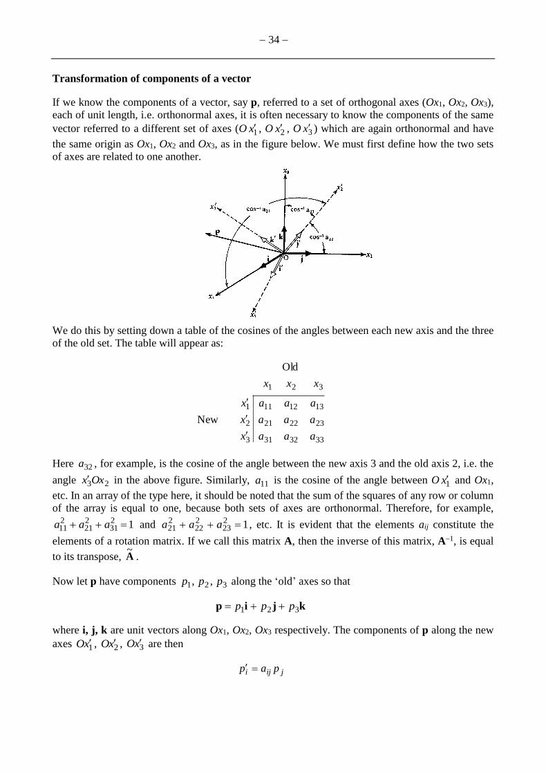
If we know the components of a vector, say p, referred to a set of orthogonal axes (Ox1, Ox2, Ox3),

each of unit length, i.e. orthonormal axes, it is often necessary to know the components of the same

vector referred to a different set of axes (O 1x , O 2x , O 3x ) which are again orthonormal and have

the same origin as Ox1, Ox2 and Ox3, as in the figure below. We must first define how the two sets

of axes are related to one another.

We do this by setting down a table of the cosines of the angles between each new axis and the three

of the old set. The table will appear as:

333231

232221

131211

3

2

1

321

New

Old

aaa

aaa

aaa

x

x

x

xxx

Here 32a , for example, is the cosine of the angle between the new axis 3 and the old axis 2, i.e. the

angle 23Oxx in the above figure. Similarly, 11a is the cosine of the angle between O 1x and Ox1,

etc. In an array of the type here, it should be noted that the sum of the squares of any row or column

of the array is equal to one, because both sets of axes are orthonormal. Therefore, for example,

1231

221

211 aaa and 12

23222

221 aaa , etc. It is evident that the elements aij constitute the

elements of a rotation matrix. If we call this matrix A, then the inverse of this matrix, A1, is equal

to its transpose, A~

.

Now let p have components 321 ,, ppp along the ‘old’ axes so that

kjip 321 ppp

where i, j, k are unit vectors along Ox1, Ox2, Ox3 respectively. The components of p along the new

axes 1xO , 2xO , 3xO are then

jiji pap

35

using dummy suffix notation. Inverting this equation, we have

ijiiijijiijj papapap )~()( 1

since the inverse of the ija matrix is its transpose.

Suppose that

jiji qTp

where the tensor T relates the vector p with components 1p , 2p and 3p to the vector q with

components 1q , 2q and 3q .

The components of the two vectors depend upon the choice of axes, because this choice determines

the values 321 ppp and 321 qqq . The vectors p and q themselves do not change. When the

axes are changed, and hence the components of p and q change, the components ijT will also

change.

If now we choose new axes i , j , k so that

jiji qTp

we then wish to find the relation between the nine components ijT and the nine components ijT .

To establish the relationship between ijT and ijT , we can perform the following mathematical

operations with suitable dummy suffices to determine the nine components of ijT :

(1) Write p in terms of p: kiki pap

(2) Write p in terms of q: lklk qTp

(3) Write q in terms of q : jjll qaq

When we combine these three operations we have

jjlkliklklikkiki qaTaqTapap

or

jjlkliki qaTap

Therefore, we have the important result

kljlikjlklikij TaaaTaT

because the order in which a product is written on the right-hand side of this equation does not

matter when the dummy suffix notation is used. This defines a tensor of the second rank, in the

sense that if an operator T relates two vectors p and q through jiji qTp , it must transform to new

axes according to this transformation.

36

Tensors of the second rank

A tensor of the second rank, ijT , is said to be symmetric if jiij TT , and to be skew symmetric or

antisymmetric if jiij TT . For our purposes, all matter tensors we are likely to encounter in

materials science are symmetric. This is also true for stress and strain field tensors.

Any symmetric tensor ijS can be transformed by a suitable choice of orthonormal axes so that it

takes on the simple form

33

22

11

00

00

00

S

S

S

i.e. all 0ijS unless ji . Such a tensor when expressed in this form is said to be referred to its

principal axes. When referred to its principal axes, the components 332211 ,, SSS are called the

principal components and are often written simply as 321 ,, SSS respectively.

Limitations imposed by crystal symmetry for second rank tensors

The discussion in this section applies to tensors used to represent physical properties of crystals,

and strictly only to perfect single crystals, i.e. ones without defects.

The fact that physical properties of crystals should remain the same when the system of coordinates

to which the properties are referred are rotated to a new set of coordinates by a symmetry operation

was first appreciated by Franz Neumann (1798–1895), a student of Christian Samuel Weiss of the

Weiss Zone Law, who applied this principle to elastic coefficients of crystals in a course in

elasticity at the University of Königsberg in 1873/4. While this is one way of defining what has

now come to be known as Neumann’s principle, it is nowadays more usual to state the principle in

the form:

‘The symmetry elements of a physical property of a crystal must include the symmetry elements of

the point group of the crystal’

It is important to appreciate that the principle does not state that the symmetry of the physical

property is the same as that of the point group: the symmetry of physical properties is often higher

than that of the corresponding point group.

Physical properties characterized by a second-order tensor are necessarily invariant with respect to

the operation of a centre of symmetry. This is implicit in the linear relations

jiji qTp

because if we substitute ip for ip and jq for jq (i.e. we reverse the directions of p and of q),

the relation is still satisfied by the same values of ijT . In terms of applying Neumann’s principle, this

means that physical properties represented by second-order tensors for all crystals must include the

symmetry of 1 ; this will be true even for crystals belonging to non-centrosymmetric point groups.

37

It will assist in understanding what follows if we look at the centre of symmetry statement in

another way. Suppose that for one set of axes (Ox1, Ox2, Ox3) the relations between the ip and the

jq are given by ijT . If we now reverse the axes of reference, leaving p and q the same as before,

this corresponds to choosing a new set of axes such that the array of the ija relating the axes is

100

0 10

0 01

New

Old

3

2

1

321

x

x

x

xxx

Here, all ija are equal to zero unless ji . We now apply the transformation formula:

kljlikij TaaT

Therefore,

1 since 332211 aaaTTaaT ijijjjiiij

What we have done here is to leave the measured quantities p and q the same and to imagine the

crystal inverted through a centre of symmetry operation. We have obtained the same result as if we

had reversed the directions of p and q.

Now suppose the crystal contains a diad axis of symmetry. If we measure a certain property along a

certain direction with respect to this axis, and then rotate the crystal 180 about this axis and

remeasure the property, we will get the same value as before by Neumann’s principle. This imposes

restrictions on the values of the components of any symmetric second-rank tensor ijS which

represents this property. In this context, it is relevant that the tensors of the second rank in which

we will be interested will all be symmetric.

To see what these restrictions are, take axes (Ox1, Ox2, Ox3) and suppose there is a diad axis along

Ox2, such as might arise in a material with monoclinic symmetry. Initially, we assume the tensor ijS

is symmetric, so that it has six independent components. Now, if we take new axes related to the

old by a rotation of 180 about Ox2, the physical property must remain the same as before. The new

axes are related to the old by the array of ija as

100

0 10

0 01

New

Old

3

2

1

321

x

x

x

xxx

38

The components of the tensor with respect to the new axes, ijS , are given in terms of the old

components, ijS , by

kljlikij SaaS

and we must have ijij SS for all i and j. If we work out the components ijS one by one we find

13133311133333333333

22222222221111111111

,

, ,

SSaaSSSaaS

SSaaSSSaaS

but

12122211122323332223 and SSaaSSSaaS

However, we must also have 2323 SS and 1212 SS . Therefore, 01223 SS . Hence, a

symmetrical second-rank tensor representing a physical property of a crystal with a two-fold axis of

rotational symmetry must have the components 23S and 12S equal to zero when referred to axes so

that Ox2 corresponds to the diad axis.

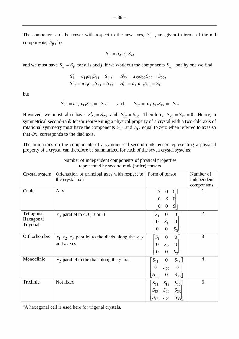
The limitations on the components of a symmetrical second-rank tensor representing a physical

property of a crystal can therefore be summarized for each of the seven crystal systems:

Number of independent components of physical properties

represented by second-rank (order) tensors

Crystal system Orientation of principal axes with respect to

the crystal axes

Form of tensor Number of

independent

components

Cubic Any

S

S

S

00

00

00

1

Tetragonal

Hexagonal

Trigonala

3x parallel to 4, 6, 3 or 3

3

1

1

00

00

00

S

S

S

2

Orthorhombic 321 ,, xxx parallel to the diads along the x, y

and z-axes

3

2

1

00

00

00

S

S

S

3

Monoclinic 2x parallel to the diad along the y-axis

3313

22

1311

0

00

0

SS

S

SS

4

Triclinic Not fixed

332313

232212

131211

SSS

SSS

SSS

6

aA hexagonal cell is used here for trigonal crystals.

39

Tensors of the second rank referred to principal axes

As we have see, when referred to its principal axes, the symmetric tensor ijS relating vectors p and

q only has its diagonal components 2211, SS and 33S as possible non-zero components. Under

these circumstances, the equations

jiji qSp

reduce to

1111 qSp , 2222 qSp , 3333 qSp .

Now let us return to the simple example of electrical conductivity. The conductivity tensor ij is

symmetric. When referred to its principal axes, all the ijσ are zero except 11σ , 22σ and 33σ . If the

crystal under consideration is orthorhombic, monoclinic or triclinic, there is no symmetry

requirement that two or more of 11σ , 22σ and 33σ have to be equal. For our purposes here we shall

assume that none of 11σ , 22σ and 33σ are equal.

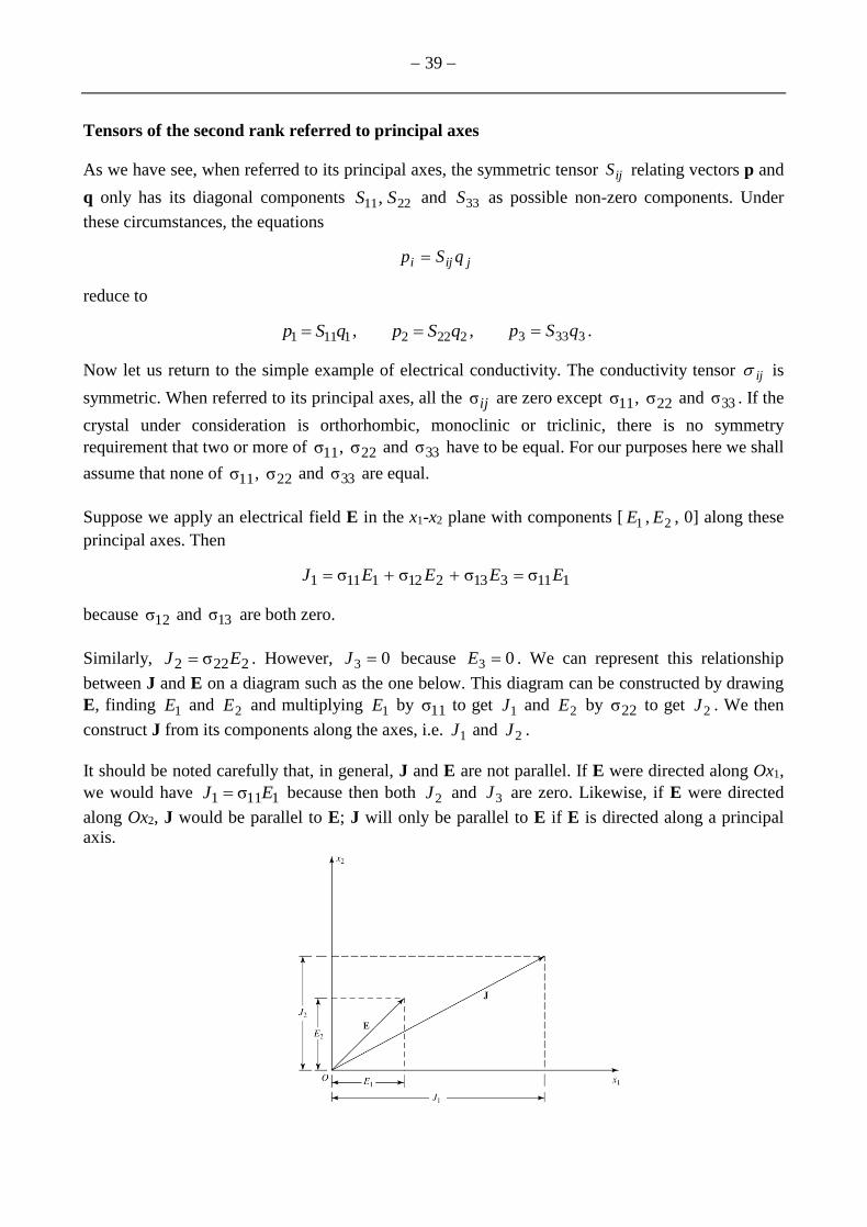
Suppose we apply an electrical field E in the x1-x2 plane with components [ 1E , 2E , 0] along these

principal axes. Then

1113132121111 σσσσ EEEEJ

because 12σ and 13σ are both zero.

Similarly, 2222 σ EJ . However, 03 J because 03 E . We can represent this relationship

between J and E on a diagram such as the one below. This diagram can be constructed by drawing

E, finding 1E and 2E and multiplying 1E by 11σ to get 1J and 2E by 22σ to get 2J . We then

construct J from its components along the axes, i.e. 1J and 2J .

It should be noted carefully that, in general, J and E are not parallel. If E were directed along Ox1,

we would have 1111 σ EJ because then both 2J and 3J are zero. Likewise, if E were directed

along Ox2, J would be parallel to E; J will only be parallel to E if E is directed along a principal

axis.

40

When we speak of the conductivity in a particular direction, what we actually mean in practice is

that if E is applied in that direction and the current density is measured in the same direction, to

give a value ||J , then the conductivity in this direction is ||J divided by the magnitude of E, i.e.

E/||J . We can find an expression for this by resolving J parallel to E.

Suppose E is applied in a direction so that its direction cosines with respect to the principal axes of

the conductivity tensor are αcos , βcos and γcos . Then we have

αcos σσ 111111 EEJ

βcos σσ 222222 EEJ

γcos σσ 333333 EEJ

where E is the magnitude of E (i.e. E ). Then, a unit vector n̂ parallel to E is simply the vector

[ αcos , βcos , γcos ] since 1γcosβcosαcos 222 . Resolving J parallel to E produces a vector

parallel to E of magnitude ||J = J. n̂ . Hence,

)γcosσβcosσαcosσ(γcosβcosαcos 233

222

211321|| EJJJJ

Therefore the conductivity in the direction parallel to E is

γcosσβcos σαcos σ/σ 233

222

211|| EJ

The steps in deriving this equation are illustrated diagrammatically in the diagram below for the

simple case where E is normal to the principal axis Ox3 of the conductivity tensor, so that 0γcos .

Derivation of the magnitude of the conductivity in a particular direction.

The figure is drawn for 11σ = 250 and 22σ = 75 ohm1 m1, so that 22σ = 0.3 11σ .

41

It is instructive to derive the result given in the box on the previous page in a different way.

Suppose we consider the meaning of the component 11 of the conductivity tensor irrespective of

whether it is referred to principal axes.

The component 11 relates the electric field along axis 1xO to the component of the current along

the same axis 1xO . If, therefore, we wish to find the value of the conductivity in a particular

direction, having been given the components of the conductivity tensor referred to its principal

axes, we can proceed as follows:

Choose a new set of axes such that 1xO is along the direction of interest. Then the component 11

of the conductivity tensor referred to this new set of axes gives us the conductivity along this

particular direction – the EJ /|| . We are only interested in 11 , so in writing out the array of the ija

for this transformation we only need to know the values of the cosines of the angles between 1xO

and the principal axes of the conductivity tensor, Ox1, Ox2 and Ox3.

Following the scheme of the expressions in the matrix of direction cosines we therefore only need

to know 1211, aa and 13a . These quantities are αcos , β cos and γcos respectively. Using the

transformation formula, we have

kljlikij aa σσ

and so when i = 1 and j = 1,

kllk aa σσ 1111

Since ijσ is defined relative to its principal axes, the only non-zero terms within this conductivity

tensor are 11σ , 22σ and 33σ . Therefore,

33131322121211111111 σσσσ aaaaaa

Substituting for 131211 ,, aaa , we obtain

γcosσβcos σαcos σσ 233

222

21111

once again.

It is clear that we could have proceeded in exactly the same way to find the conductivity in a

particular direction, even if the values of the components of ijσ , the conductivity tensor, had not

been given to us referred to principal axes. In this case there would have been, in general, nine

terms in the expansion of kljlikij aa σσ . This transformation formula clearly holds irrespective of

whether the ijσ are referred to principal axes.

42

Therefore, we can state that to find the value of a property of a crystal in a particular direction we

proceed as follows:

Let the components of the tensor representing this property be given as ijT referred to axes (Ox1,

Ox2, Ox3). Choose an axis along the direction of interest and call this 1xO . Let this axis have

direction cosines referred to (Ox1, Ox2, Ox3) of a11, a12, a13 respectively. Then the value of the

property 11T in the direction we are interested in is given by

ijji TaaT 1111

This relation holds for all second-rank tensors whether or not they are symmetrical. This equation

can be written in a convenient shorthand notation by removing the dash and the ‘1’ subscripts in

this equation, so that the property T along the direction of interest is

ijji TllT

where the relevant direction cosines are now defined as l1, l2 and l3 to conform to the notation used

by Nye.

Representation quadric

The equation

γcosσβcos σαcos σσ 233

222

21111

is that of a general surface of the second degree referred to its principal axes, taking in general the

form

γcosβcosαcos1 222

2CBA

r

which is of the same form as the equation for 11σ . As a consequence, the variation of a given

property of a crystal with direction, can be represented by a suitable figure in three-dimensional

space. When all the values of the property are positive, as in the case of electrical conductivity, this

second-degree surface, or representation quadric, is an ellipsoid.

If in general we construct an ellipsoid of semi-principal axes 321 /1,/1,/1 SSS , as in the figure

on the next page, so that a general point on the ellipsoid satisfies the equation

1233

222

211 xSxSxS

then the length r of any radius vector of the ellipsoid (representation quadric) is equal to the

reciprocal of the square root of the magnitude of the property S in that direction.

Returning to the example of electrical conductivity, and we know the values 1σ , 2σ and 3σ of the

components of the electrical conductivity referred to principal axes, then we can construct the

ellipsoid defining the conductivity quadric.

43

If now a field E is applied in any direction, the magnitude of the conductivity in that direction can

be found by drawing a radius vector r in the direction of E, measuring the value of r and taking the

reciprocal of the square root of r to find the conductivity in that direction.

Radiusnormal property of the representation quadric

The representation ellipsoid has a further very useful property known as the radius–normal

property. It can be stated as follows: if ijS are the components of a symmetrical second-rank tensor

relating the vectors p and q so that jiji qSp , then the direction of p for a given q can be found by

drawing a radius vector OQ of the representation quadric parallel to q and finding the normal to the

quadric at Q. This is shown in two dimensions in the figure below.

The radius-normal property of a representation ellipsoid

A proof of this property is given in Section 5.9 of Kelly and Knowles.

p

q

O

Q

44

Third and fourth-rank tensors

Just as a second-rank tensor relates two vectors, so a third-rank tensor relates a second-rank tensor

and a vector, and a fourth-rank tensor relates two second-rank tensors, and so on. Thus, for a tensor

of the third rank ijkT , such as the piezoelectric tensor, we can envisage a relationship between a

second rank tensor jkσ and a vector ip so that, for example,

jkijki Tp σ

Equally, relationships could be of the general form

kijkij pTσ

where we require the tensor of the third rank to transform as

lmnknjmilijk TaaaT

generalising the result for a tensor of the second rank. Likewise, a tensor of the fourth rank ijklT

such as the stiffness tensor ijklc and the compliance tensors ijkls , can relate two tensors of the

second rank, ijσ and klg through an equation of the form

klijklij gTσ

where ijklT transforms as

mnpqlqkpjnimijkl TaaaaT

We are now in a position to examine the relationship between the stress and strain field tensors.

Further aspects not considered here considering the effects of crystal symmetry on third and fourth

rank tensors are discussed in the book by Kelly and Knowles.

45

Infinitesimal strain

This is relevant for a description of how elastic strains affect perfect crystals when considering both

piezoelectricity and elasticity

The distortion of a body can be described by giving the displacement of each point from its location

in the undistorted state. Any displacements which do not correspond to a translation or rotation of

the body as a whole will produce a strain.

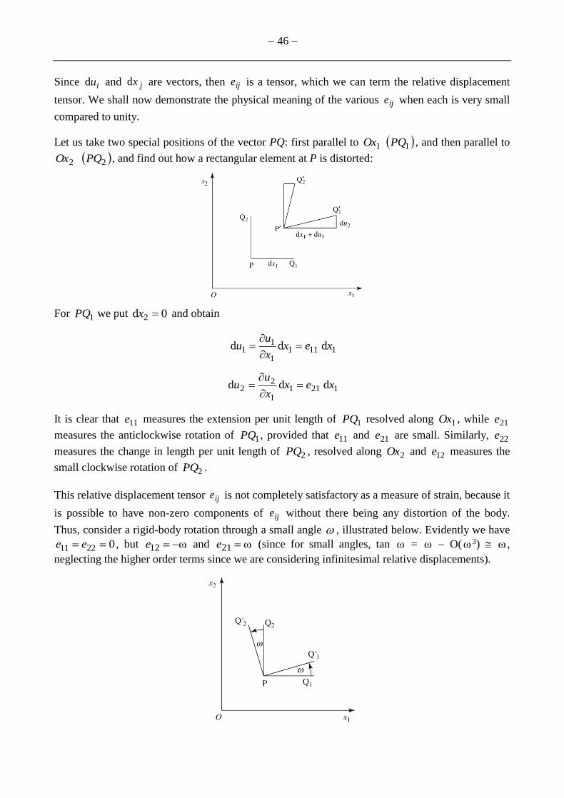
If we confine ourselves to two dimensions, we can choose an origin fixed in space such as O in the

diagram below. Let P be a point with coordinates ( 21, xx ) in the unstrained state, which after

distortion of the body moves to the point P . (Then the displacement of the point P is the vector

PP .) Let the coordinates of P be ( 2211 , uxux ).

Now consider a point Q with coordinates ( 2211 d,d xxxx ) lying infinitesimally close to P in the

unstrained state. After deformation Q moves to Q . Now, in a strained body the displacement of Q

will not be exactly the same as that of P. The displacement of Q to Q has components

( 2211 d,d uuuu ). We can write

22

11

1

11 ddd x

x

ux

x

uu

and

22

21

1

22 ddd x

x

ux

x

uu

Defining the four quantities at the point P,

1

221

2

222

2

112

1

111 ,,,

x

ue

x

ue

x

ue

x

ue

,

all of which can be compactly written as

2,1dd jxeu jiji

46

Since iud and jxd are vectors, then ije is a tensor, which we can term the relative displacement

tensor. We shall now demonstrate the physical meaning of the various ije when each is very small

compared to unity.

Let us take two special positions of the vector PQ: first parallel to 1Ox 1PQ , and then parallel to

2Ox 2 PQ , and find out how a rectangular element at P is distorted:

For 1PQ we put 0d 2 x and obtain

11111

11 ddd xex

x

uu

12111

22 ddd xex

x

uu

It is clear that 11e measures the extension per unit length of 1PQ resolved along 1Ox , while 21e

measures the anticlockwise rotation of 1PQ , provided that 11e and 21e are small. Similarly, 22e

measures the change in length per unit length of 2PQ , resolved along 2Ox and 12e measures the

small clockwise rotation of 2PQ .

This relative displacement tensor ije is not completely satisfactory as a measure of strain, because it

is possible to have non-zero components of ije without there being any distortion of the body.

Thus, consider a rigid-body rotation through a small angle , illustrated below. Evidently we have

02211 ee , but ω12 e and ω21 e (since for small angles, tan ω = ω O(ω 3) ω ,

neglecting the higher order terms since we are considering infinitesimal relative displacements).

47

To remove the component of rotation from a general ije we express it as the sum of a symmetrical

tensor, ijε , and an antisymmetrical tensor, ijω , so that

jiijjiijijijij eeeee 2

1

2

1ωε

Then jiijij ee 2

1ε is defined as the pure strain and jiijij ee 2

1ω measures the rotation.

The shear component of the pure strain tensor 12 is half the engineering shear strain γ (see Kelly

and Knowles for further details).

In specifying infinitesimal strain in three dimensions, the result is

33233221

133121

322321

22122121

311321

211221

11

332313

232212

131211

εεε

εεε

εεε

eeeee

eeeee

eeeee

The diagonal components of ij are the changes in length per unit length of lines parallel to the

axes and are called the tensile strains. The off-diagonal components measure shear strains so that,

for instance, 13 is one-half the change in angle between two lines originally parallel to the 1Ox

and 3Ox axes.

Since pure strain is a symmetrical second-rank tensor, it can be referred to principal axes. Under

these circumstances, the shear components vanish and we then have

3

2

1

ε00

0ε0

00ε

ε

The components of a given strain transform according to the general transformation law

kljlikij aa εε

48

Stress

The stress tensor is also a symmetric tensor when a material in equilibrium, and so in general it can

be represented in the form

332313

232212

131211

σσσ

σσσ

σσσ

σ

Therefore, when the axes of reference are rotated, the components of a given stress transform

according to the general transformation law

kljlikij aa σσ

Since the stress tensor is symmetrical ( jiij σσ ), it is always possible to find a set of axes, the

principal axes, so that a cube with its edges parallel to them has no shear stresses acting upon its

faces. Referred to the principal axes, the stress takes the form

3

2

1

σ00

0σ0

00σ

where 21 σ,σ and 3σ are called the principal stresses.

Elasticity of crystals

The most general linear dependence of stress on strain has the form

klijklij c εσ

The constants ijklc are called stiffness constants. The existence of non-zero values of certain of the

ijklc has rather surprising consequences. For example, if 1112c is not zero, the occurrence of a finite

shear strain 12ε implies the existence of a proportional tensile stress 11σ . By symmetry arguments,

it can be shown that constants of the type 1112c are zero in an isotropic medium, but they are in

general not zero in a single crystal. The existence of a single strain component in a crystal may

require that there be non-zero values of all the stress components.

Similarly,

klijklij s σε

where the constants ijkls are called compliances.

49

As these two formulae both consist of nine equations, each containing nine terms on the right-hand

side, it might appear that 81 compliances or stiffness constants must be specified. However, the

number of independent constants can always be reduced from 81 to 21.

Since 2112 , the constants 12ijc and 21ijc always occur together in 122112 ε σ ijijij cc . It is

therefore permissible to set 2112 ijij cc , and, in general, ijlkijkl cc . Next, suppose that only the

strain component 11ε exists. We have

11121112 εσ c

and

11211121 εσ c

Because 211112112112 ,σσ cc and in general jiklijkl cc . Similar arguments apply to the ijkls .

The number of independent constants is now reduced to 36, and so we can use the contracted

notation for stress and a contracted notation for strain where

3421

521

421

2621

521

621

1

332313

232212

131211

(note the factors of 21 , explained in Kelly and Knowles).

A corresponding contraction is applied to ijklc , so that, for example,

442332442323631233 ,, cccccc , etc. Hence the formulae klijklij c εσ can now be written

in the contracted form

jiji c

Factors of 2 and 4 must also be introduced into the definition of ijs , as follows:

ijklmn ss 2 when one only of either m or n is 4, 5 or 6

ijklmn ss 4 when both m and n are 4, 5 or 6

For example, 113313 ss , 112314 2ss and 231246 4ss . With these definitions, the formulae

klijklij s σε can be written as

jiji s

The fact that the energy stored in an elastically strained crystal depends on the strain, and not on the

path by which the strained state is reached, makes jiij cc and jiij ss , reducing to 21 the

maximum number of non-zero ijc and ijs (see for example, Section 6.5 of Kelly and Knowles).

50

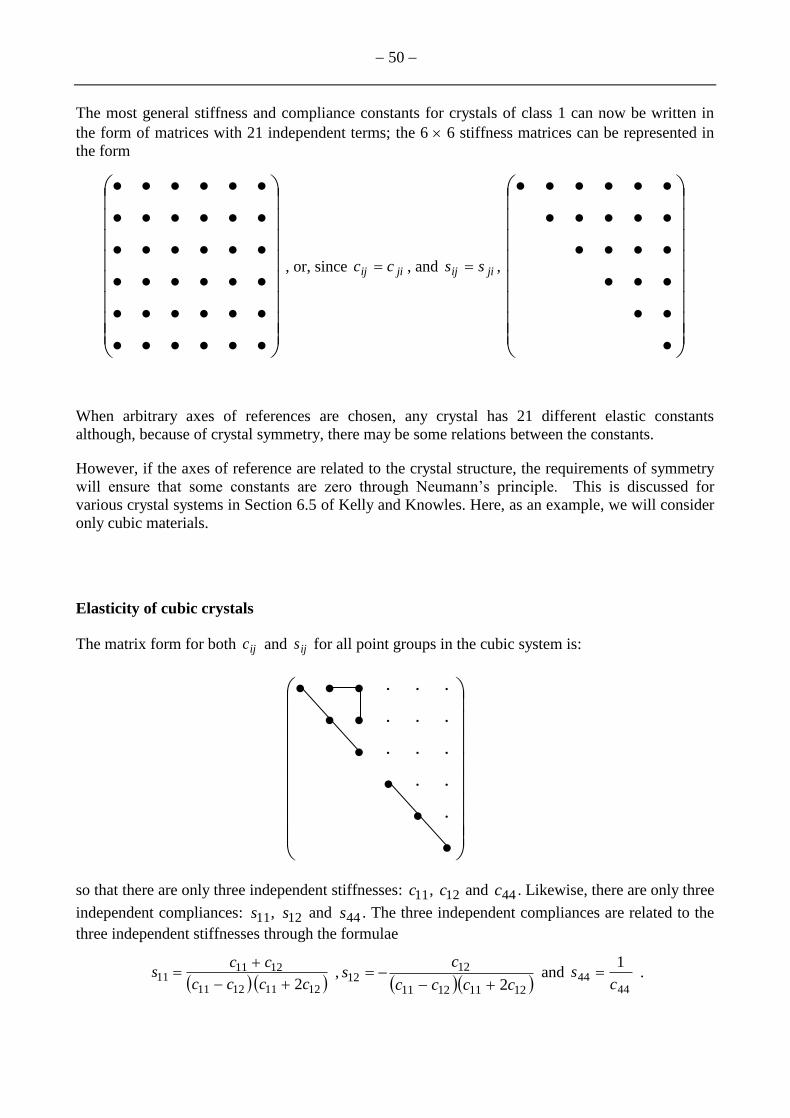
The most general stiffness and compliance constants for crystals of class 1 can now be written in

the form of matrices with 21 independent terms; the 6 6 stiffness matrices can be represented in

the form

, or, since jiij cc , and jiij ss ,

When arbitrary axes of references are chosen, any crystal has 21 different elastic constants

although, because of crystal symmetry, there may be some relations between the constants.

However, if the axes of reference are related to the crystal structure, the requirements of symmetry

will ensure that some constants are zero through Neumann’s principle. This is discussed for

various crystal systems in Section 6.5 of Kelly and Knowles. Here, as an example, we will consider

only cubic materials.

Elasticity of cubic crystals

The matrix form for both ijc and ijs for all point groups in the cubic system is:

so that there are only three independent stiffnesses: 11c , 12c and 44c . Likewise, there are only three

independent compliances: 11s , 12s and 44s . The three independent compliances are related to the

three independent stiffnesses through the formulae

12111211

121111

2cccc

ccs

,

12111211

1212

2cccc

cs

and

4444

1

cs .

51

In an isotropic medium, the elastic constants must be independent of the choice of coordinate axes.

This requirement imposes an extra condition in addition to the conditions of cubic symmetry, which

can be shown to be the condition

1211442 ccc

or equivalently,

121144 2 sss

The degree of anisotropy of a cubic single crystal can be measured by the departure from unity of

the ratio A, where

44

1211

1211

44 22

s

ss

cc

cA

The ratio A is a measure of the relative resistance of the crystal to two types of shear strain: 44c is a

measure of the resistance to shear on the (010) plane in the [001] direction, while 121121 cc is

the stiffness with respect to shear on (110) in the direction [ 011 ]. Only single crystals of W and Al

come close to being isotropic.

If we now look at cubic materials in a bit more detail, it is possible to drive the following very

useful general results:

The ijklC transform from axes 1, 2 and 3 to the axes 1', 2' and 3' so that in general

lukujuiujkiljlikklijijkl aaaacccc cC )2()δδδδ(δδ 4412114412

where the dummy suffix u takes the values 1, 2 and 3 and where is the Kronecker delta. Likewise,

for the same change in axes,

lukujuiujkiljlikklijijkl aaaassss

sS )()δδδδ(4

δδ 442

11211

4412

Thus, for example,

)( )2( 223

233

222

232

221

231441211443232 aaaaaaccccC

)( )2

(4

223

233

222

232

221

231

441211

443232 aaaaaa

sss

sS

52

Shear elastic constants 44c on the (111) plane of cubic crystals

Suppose we were interested in the variation of the elastic constants 44c on the (111) plane. We

might choose out ‘3’ axis to be the normal to the (111) plane, leaving us two axes ‘1’ and ‘2’ to

define in this plane.

Since the plane of interest is (111), it follows that 3/1333231 aaa . Hence,

)(3

1)( )2(

3

1441211

233

232

22144121144443232 cccaaacccccC

since 1)( 233

232

221 aaa irrespective of how we define our ‘2’ and ‘1’ axes. Therefore, we have

immediately the result that the 44c shear elastic constant of cubic materials is isotropic in the (111)

plane. It also follows that the 44s shear elastic constant of cubic materials is also isotropic in the

(111) plane, as is the shear modulus 44/1 sG on this plane.

Young’s modulus as a function of orientation in cubic crystals

A second useful result is the formula for Young’s modulus, E, as a function of orientation. From the

formula for ijklS , we have:

)( )(2

413

412

411442

11211

4412111111 aaasss

s ssS

or, equivalently,

)( )( 2 211

213

213

212

212

211442

112111111 aaaaaasss ss

so that 11/1 sE .

If ‘1’ is along <111>, we have 3/1213

212

211 aaa , so that

)2( 3

1 )(

3

2441211442

112111111 ssssss ss

whence

)2(

3

441211 sssE

Along <100>,

11

1

sE

Using these formulae, it is easy to show that cubic metals with A > 1 are most stiff along <111>

directions and least stiff along <001> directions; the reverse is true for cubic metals with A < 1.