lecture 31 analysis of covariance - purdue...
TRANSCRIPT

31-1
Lecture 31
Analysis of Covariance
STAT 512
Spring 2011
Background Reading
KNNL: Chapter 22

31-2
Topic Overview
• Covariates; a couple of extreme examples
• ANCOVA
• “Adjusted” or Least-Squares Means

31-3
Analysis of Covariance
• ANCOVA is really “ANOVA with
covariates” or, more simply, a combination
of ANOVA and regression
• Use when you have some categorical factors
and some quantitative predictors.
Continuous variables are referred to as
covariates or concomitant variables.

31-4
Analysis of Covariance (2)
• Similar to blocking - the idea is that
concomitant variables are not necessarily
of primary interest, but still their inclusion
in the model will help explain more of the
response, and hence reduce the error
variance.
• In some situations, failure to include an
important covariate can yield misleading
results.

31-5
Example #1
• Studying three potential treatments of an
aggressive form of cancer.
• Response variable is the number of months a
patient lives after being placed on a
treatment.
• We will analyze the data as a one-way
ANOVA (see ancova.sas for code).

31-6

31-7
ANOVA Results
Sum of
Source DF Squares Mean Square F Value Pr > F
TRT 2 1131.555556 565.777778 22.94 0.0015
Error 6 148.000000 24.666667
Total 8 1279.555556
• Seems clear there is a significant treatment
effect, right?
y LSMEAN trt Number
A 40.66667 1 1
B 24.66667 2 2
B
B 13.33333 3 3

31-8
ANOVA Results (2)
• The analysis tells us that there is a
significant treatment effect. It suggests
that Treatment 1 is clearly the best (since
people live longer).
• So we put a large group of people on
Treatment 1 expecting them to live 40+
months, but unfortunately they do not live
this long. What did we do wrong????

31-9
The oversight...
• Consider the stage to which the cancer has
progressed at the time that treatment
begins.
• This is important, because those at earlier
stages of disease will naturally live longer
on average.
• The following plot illustrates where things
went awry:

31-10

31-11
Lifetime vs Duration
• There is clearly a linear relationship between
the duration of the cancer and the length of
time someone has left to live.
• Furthermore, we notice from the plot that
the group assigned to the first treatment
were all in an earlier stage of the disease,
those assigned to the second treatment
were all in a middle stage, and those
assigned to the third treatment were all in a
later stage.

31-12
Treatment Effects?
• After seeing this plot, it is clear that we can’t compare the lifetimes without considering the
duration of the disease.
• We would suspect looking at this plot to find the
treatments are not all that different. The
following ANCOVA output leads to that
conclusion:
Source DF SS Mean Square F Value Pr > F
x 1 1225.166536 1225.166536 199.15 <.0001
trt 2 23.628758 11.814379 1.92 0.2405
Error 5 30.760262 6.152052
Total 8 1279.555556

31-13
MEANS vs. LSMEANS • The MEANS statement compares the
unadjusted means – for this problem that is
WRONG. This was the original output we
considered, where Treatment 1 appeared to
be the best.
• The LSMEANS statement adjusts for any
concomitant variables in the model. You
can think of the LSMEAN for a given
treatment as the “mean response for that
treatment, at the AVERAGE value(s) of
the covariate(s)”

31-14
MEANS vs. LSMeans (2)
trt N Mean LSMEAN LSMEAN #
1 3 40.67 26.09 1
2 3 24.67 23.91 2
3 3 13.33 28.67 3
y LSMEAN trt Number
A 28.67261 3 3
A
A 26.08623 1 1
A
A 23.90783 2 2
31-15
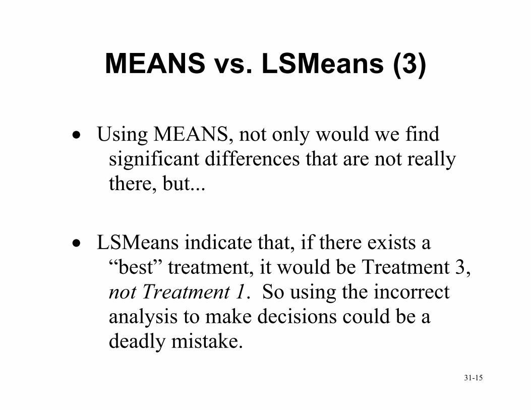
MEANS vs. LSMeans (3)
• Using MEANS, not only would we find
significant differences that are not really
there, but...
• LSMeans indicate that, if there exists a
“best” treatment, it would be Treatment 3,
not Treatment 1. So using the incorrect
analysis to make decisions could be a
deadly mistake.

31-16
Conclusions
• Stage of disease is the contributing factor
toward lifetime – it really didn’t have
anything to do with the choice of
treatment.
• It just happened that everyone on treatment
1 was in an earlier stage of the disease and
so that made it look like there was a
treatment effect. In fact, if we were to
recommend a treatment, we might prefer
Treatment #3 (although there is no sig.
difference among any of the treatments).

31-17
A Second Example
• It is also possible to have a difference in
means, but not be able to see it unless you
first adjust for a covariate.
• Consider the same type of setting as where
we want to test the effect of treatment on
cancer, but with different data.

31-18
31-19
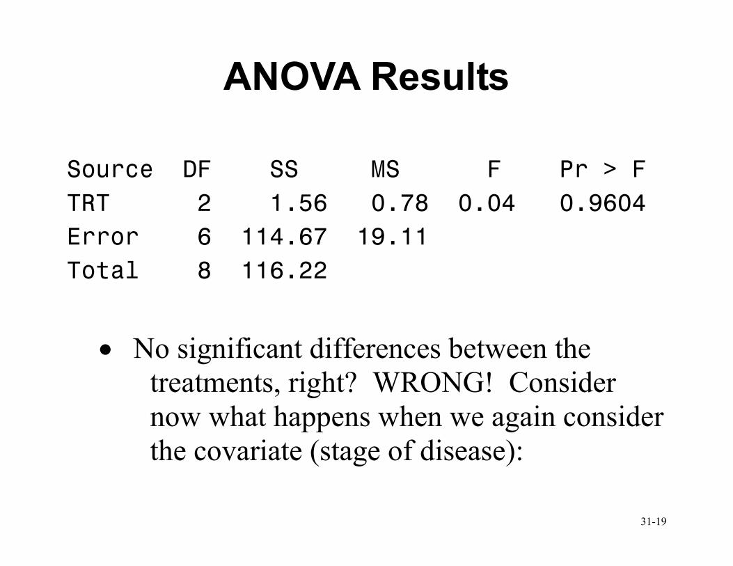
ANOVA Results
Source DF SS MS F Pr > F
TRT 2 1.56 0.78 0.04 0.9604
Error 6 114.67 19.11
Total 8 116.22
• No significant differences between the
treatments, right? WRONG! Consider
now what happens when we again consider
the covariate (stage of disease):
31-20

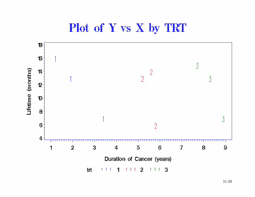
31-21
Covariate
• Again all taking Treatment 1 were in the
early stages of the disease, all on
Treatment 2 in the middle stages, and all
on Treatment 3 in the latter stages.
• Is there a treatment effect? Treatment 3
appears to be keeping those at advanced
stages of disease alive equally as long as
Treatment 1 does for those in early stages.
Surely Treatment 3 is better.

31-22
ANCOVA
Source DF SS MS F Value Pr > F
Time 1 6.98 6.98 1.11 0.3407
trt 2 77.77 38.88 6.18 0.0446
Error 5 31.48 6.30
Total 8 116.22
• Note that duration of the cancer by itself
appears insignificant (if we look at Type I
SS).

31-23
ANCOVA (2) • We must realize that the duration of the
cancer at time of treatment IS important
and MUST be included in the model – or
we get mistaken results. We must adjust
for it before we can see the differences in
treatments.
• Note: the duration actually will test as
important, but we cannot see it here until
the treatments are in the model (see Type
III sums of squares).

31-24
LSMEANS
y LSMEAN trt Number
A 26.269579 3 3
B 11.984466 2 2
B
B -3.587379 1 1

31-25
Conclusions
• The output indicates that Treatment #3 is significantly better than the other two
treatments.
• This time the potentially deadly mistake would be to assume based on a one-way ANOVA
that the treatments were equivalent and use
the cheapest one (unless you were lucky and
that was Treatment #3)
• Note that these examples were just for illustration – in reality, one should redesign
this experiment and collect more data.

31-26
Data for one-way ANCOVA
• Yij is the jth observation on the response
variable in the ith group
• Xij is the jth observation on the covariate in
the ith group
• i = 1, . . . , r levels (groups) of factor
• j = 1, . . . , ni observations for level i
31-27
Basic ideas behind ANCOVA
• Covariates (concomitant variables) can
reduce the MSE, thereby increasing power
for testing. And as we have seen,
sometimes they are absolutely necessary in
order to get accurate analysis.
• A covariate can adjust for differences in
characteristics of subjects in the treatment
groups. Baseline or pretest values are
often used as covariates.

31-28
Assumptions
• Ideally the covariate will not be in any way
related to the treatment variables (factors).
• We assume that the covariate will be
linearly related to the response and that the
relationship will be the same for all levels
of the factor (no interaction between
covariate and factor).

31-29
Cell Means Model
( )ij i ij ijY X Xµ β ε= + − +ii
• As usual ( )2~ 0,iid
ij Nε σ
• ( )( )2~ ,ij i ijY N X Xµ β σ+ −ii
, independent
• For each i, we have a simple linear
regression in which the slopes are the
same, but the intercepts may differ (i.e.
different means once covariate has been
“adjusted” out).

31-30
Parameters
• The parameters of the model are 2
1 2, ,..., , ,rµ µ µ β σ .
• We use multiple regression methods to
estimate the iµ and β
• We use the residuals from the model to
estimate 2σ (via the MSE)

31-31
Factor Effects Model
( )ij i ij ijY X X= µ +α +β − + εii
• Again, ( )2~ 0,iid
ij Nε σ
• Constraints: 0iα =∑ (or in SAS 0aα = )
• Expected value of a Y with level i and
ijX x= is ( )i x Xµ + α +β −ii
• Note: the difference i iα α ′− does NOT
dependent on the value of x.
31-32
LSMeans
• LSMEAN for treatment i is the expected
value of a Y with level i and ijX x=ii
• Value of LSMEAN for treatment i is
i xµ α β+ +ii
• Also known as the adjusted estimated
treatment mean.

31-33
SAS LSMeans Statement
• STDERR gets the standard errors for the least-square means
• TDIFF requests the matrix of statistics (with p-values) that will do pairwise comps.
PDIFF gets the p-values
• For multiple comparison procedures, add ADJUST=<type> where <type> can be
TUKEY, BON, SCHEFFE, DUNNETT
• CL gets confidence limits for the means (and differences in conjunction with PDIFF).

31-34
Crackers Example
(crackers.sas)
• Y is then number of cases of crackers sold
during promotion period
• Factor is the type of promotion (r=3)
� 1 = customers sample in store
� 2 = added shelf space
� 3 = special display cells
• ni = 5 different stores per type
• The covariate X is the number of cases of
crackers sold in the preceding period.

31-35

31-36
Analysis in SAS
proc glm data=a1; class promo; model cases=last promo /solution clparm; lsmeans promo /adjust=tukey stderr tdiff pdiff cl; run;
Reminder: Check assumptions!

31-37
Output
Source DF SS MS F Pr > F
last 1 190.68 190.68 54.38 <.0001
promo 2 417.15 208.58 59.48 <.0001
Error 11 38.57 3.51
Total 14 646.40
R-Square 0.940329
Source DF SS-III MS F Value Pr > F
last 1 269.03 269.03 76.72 <.0001
promo 2 417.15 208.58 59.48 <.0001

31-38
Parameter EST SE T-value
Intercept 12.28 B 2.83 4.33
last 0.90 0.10 8.76
promo samples 5.08 B 1.23 4.13
promo spcshlf -7.90 B 1.19 -6.65
promo xtrshlf 0.00 B . .
Parameter Pr > |t| 95% CL __
Intercept 0.0012 6.04 18.52
last <.0001 0.67 1.12
promo samples 0.0017 2.37 7.78
promo spcshlf <.0001 -10.52 -5.29
promo xtrshlf . . .

31-39
promo LSMEAN SE Pr > |t| LSMEAN#
samples 39.82 0.858 <.0001 1
spcshlf 26.84 0.838 <.0001 2
xtrshlf 34.74 0.850 <.0001 3
i/j 1 2 3
1 <.0001 0.0044
2 <.0001 <.0001
3 0.0044 <.0001
promo LSMEAN 95% Confidence Limits
samples 39.82 37.93 41.70
spcshlf 26.84 25.00 28.69
xtrshlf 34.74 32.87 36.61

31-40
Conclusions
• Providing Samples is the most effective
sales tactic (significantly better than the
other two)
• Extra shelf space devoted to an item is more
effective than a special display
. .

31-41
Conclusions (2)
• Common slope is 0.9. The option ‘clparm’
can be used to get confidence intervals on
the parameters. Note however that only
CI’s for UNBIASED estimates (in this
case the slope for LAST) are appropriate.
The 95% CI for the slope was found to be
(0.67,1.12).
• Note: Might have done this analysis by
analyzing the difference in cases sold
(single factor ANOVA)

31-42
Upcoming in Lecture 32...
• Two-way Analysis of Covariance
• More Examples