lecture 4 - hidden markov models -...
TRANSCRIPT

Lecture 4Hidden Markov Model (HMM)
Yossi Keshet
Based on the slides of Michael Picheny, Bhuvana Ramabhadran, and Stanley F.
Chen presented at the speech recognition course e6870 given at Colombia
University Fall 2012.

Introduction to Hidden Markov Models
The issue of weights in DTW.Interpretation of DTW grid as Directed Graph.Adding Transition and Output Probabilities to the Graphgives us an HMM!The three main HMM operations.
100 / 113

Another Issue with Dynamic Time Warping
Weights are completely heuristic!Maybe we can learn weights from data?Take many utterances . . .
101 / 113

Learning Weights From Data
For each node in DP path, count number of times move up" right ! and diagonally %.Normalize number of times each direction taken by totalnumber of times node was actually visited.Take some constant times reciprocal as weight.Example: particular node visited 100 times.
Move % 50 times; ! 25 times; " 50 times.Set weights to 2, 4, and 4, respectively (or 1, 2, and 2).
Point: weight distribution should reflect . . .Which directions are taken more frequently at a node.
Weight estimation not addressed in DTW . . .But central part of Hidden Markov models.
102 / 113

DTW and Directed Graphs
Take following Dynamic Time Warping setup:
Let’s look at representation of this as directed graph:
103 / 113

DTW and Directed Graphs
Another common DTW structure:
As a directed graph:
Can represent even more complex DTW structures . . .Resultant directed graphs can get quite bizarre.
104 / 113

Path Probabilities
Let’s assign probabilities to transitions in directed graph:
aij is transition probability going from state i to state j ,where
Pj aij = 1.
Can compute probability P of individual path just usingtransition probabilities aij .
105 / 113

Path Probabilities
It is common to reorient typical DTW pictures:
Above only describes path probabilities associated withtransitions.Also need to include likelihoods associated withobservations.
106 / 113

Path Probabilities
As in GMM discussion, let us define likelihood of producingobservation xi from state j as
bj(xi) =X
m
cjm1
(2⇡)d/2|⌃jm|1/2 e�12 (x
i
�µjm)T ⌃�1jm (x
i
�µjm)
where cjm are mixture weights associated with state j .This state likelihood is also called the output probabilityassociated with state.
107 / 113

Path Probabilities
In this case, likelihood of entire path can be written as:
108 / 113

Hidden Markov Models
The output and transition probabilities define a HiddenMarkov Model or HMM.
Since probabilities of moving from state to state onlydepend on current and previous state, model is Markov.Since only see observations and have to infer statesafter the fact, model is hidden.
One may consider HMM to be generative model of speech.Starting at upper left corner of trellis, generateobservations according to permissible transitions andoutput probabilities.
Not only can compute likelihood of single path . . .Can compute overall likelihood of observation string . . .As sum over all paths in trellis.
109 / 113

HMM: The Three Main Tasks
Compute likelihood of generating string of observationsfrom HMM (Forward algorithm).Compute best path from HMM (Viterbi algorithm).Learn parameters (output and transition probabilities) ofHMM from data (Baum-Welch a.k.a. Forward-Backwardalgorithm).
110 / 113

Simplification: Discrete Sequences
Goal: continuous data.
e.g., P(x1
, . . . , xT ) for x 2 R40
.
Most of today: discrete data.
P(x1
, . . . , xT ) for x 2 finite alphabet.
Discrete HMM’s vs. continuous HMM’s.
9 / 130

Vector Quantization
Before continuous HMM’s and GMM’s (⇠1990) . . .
People used discrete HMM’s and VQ (1980’s).
Convert multidimensional feature vector . . .
To discrete symbol {1, . . . , V} using codebook.
Each symbol has representative feature vector µj .
Convert each feature vector . . .
To symbol j with nearest µj .
10 / 130

The Basic Idea
How to pick the µj?
µ1
µ2
µ3
µ4
µ5
11 / 130

The Basic Idea
µ1
µ2
µ3
µ4
µ5
x
1
x
2
x
3
x
4
x
5
x
6
x
1
, x
2
, x
3
, x
4
, x
5
, x
6
. . .) 4, 2, 2, 5, 5, 5, . . .
12 / 130

Recap
Need probabilistic sequence modeling for ASR.
Let’s start with discrete sequences.
Simpler than continuous.
What was used first in ASR.
Let’s go!
13 / 130

Part I
Nonhidden Sequence Models
14 / 130

Case Study: Coin Flipping
Let’s flip (unfair) coin 10 times: x1
, . . . x10
2 {T, H}, e.g.,T, T, H, H, H, H, T, H, H, H
Design P(x1
, . . . xT ) matching actual frequencies . . .
Of sequences (x1
, . . . xT ).
What should form of distribution be?
How to estimate its parameters?
15 / 130

Where Are We?
1
Models Without State
2
Models With State
16 / 130

Independence
Coin flips are independent !Outcome of previous flips doesn’t influence . . .
Outcome of future flips (given parameters).
P(x1
, . . . x10
) =10Y
i=1
P(xi)
System has no memory or state.
Example of dependence: draws from deck of cards.
e.g., if last card was A�, next card isn’t.
State: all cards seen.
17 / 130

Modeling a Single Coin Flip P(xi)
Multinomial distribution.
One parameter for each outcome: pH , pT � 0 . . .
Modeling frequency of that outcome, i.e., P(x) = px .
Parameters must sum to 1: pH + pT = 1.
Where have we seen this before?
18 / 130

Computing the Likelihood of Data
Some parameters: pH = 0.6, pT = 0.4.
Some data:
T, T, H, H, H, H, T, H, H, H
The likelihood:
P(x1
, . . . x10
) =10Y
i=1
P(xi) =10Y
i=1
pxi
= pT ⇥ pT ⇥ pH ⇥ pH ⇥ pH ⇥ · · ·= 0.67 ⇥ 0.43 = 0.00179
19 / 130

Computing the Likelihood of Data
More generally:
P(x1
, . . . xN) =NY
i=1
pxi
=Y
x
pc(x)x
log P(x1
, . . . xN) =X
x
c(x) log p(x)
where c(x) is count of outcome x .
Likelihood only depends on counts of outcomes . . .
Not on order of outcomes.
20 / 130

Estimating Parameters
Choose parameters that maximize likelihood of data . . .
Because ML estimation is awesome!
If H heads and T tails in N = H + T flips, log likelihood is:
L(xN1
) = log(pH)H(pT )T = H log pH + T log(1� pH)
Taking derivative w.r.t. pH and setting to 0.
HpH� T
1� pH= 0 pH =
HH + T
=HN
H � H ⇥ pH = T ⇥ pH pT = 1� pH =TN
21 / 130

Maximum Likelihood Estimation
MLE of multinomial parameters is intuitive estimate!
Just relative frequencies: pH = HN , pT = T
N .
Count and normalize, baby!
0
HN 1
P(x
N1
)
pH
22 / 130

Example: Maximum Likelihood Estimation
Training data: 50 samples.
T, T, H, H, H, H, T, H, H, H, T, H, H, T, H, H, T, T, T, T, H,
T, T, H, H, H, H, H, T, T, H, T, H, T, H, H, T, H, T, H, H, H,
T, H, H, T, H, H, H, T
Counts: 30 heads, 20 tails.
pMLE
H =30
50
= 0.6 pMLE
T =20
50
= 0.4
Sample from MLE distribution:
H, H, T, T, H, H, H, T, T, T, H, H, H, H, T, H, T, H, T, H, T,
T, H, T, H, H, T, H, T, T, H, T, H, T, H, H, T, H, H, H, H, T,
H, T, H, T, T, H, H, H
23 / 130

Recap: Multinomials, No State
Log likelihood just depends on counts.
L(xN1
) =X
x
c(x) log px
MLE: count and normalize.
pMLE
x =c(x)
N
Easy peasy.
24 / 130

Where Are We?
1
Models Without State
2
Models With State
25 / 130

Case Study: Austin Weather
From National Climate Data Center.
R = rainy = precipitation > 0.00 in.
W = windy = not rainy; avg. wind � 10 mph.
C = calm = not rainy and not windy.
Some data:
W, W, C, C, W, W, C, R, C, R, W, C, C, C, R, R, R, R, C,
C, R, R, R, R, R, R, R, R, C, C, C, C, C, R, R, R, R, R,
R, R, C, C, C, W, C, C, C, C, C, C, R, C, C, C, C
Does system have state/memory?
Does yesterday’s outcome influence today’s?
26 / 130

State and the Markov Property
How much state to remember?
How much past information to encode in state?
Independent events/no memory: remember nothing.
P(x1
, . . . , xN)?=
NY
i=1
P(xi)
General case: remember everything (always holds).
P(x1
, . . . , xN) =NY
i=1
P(xi |x1
, . . . , xi�1
)
Something in between?
27 / 130

The Markov Property, Order n
Holds if:
P(x1
, . . . , xN) =NY
i=1
P(xi |x1
, . . . , xi�1
)
=NY
i=1
P(xi |xi�n, xi�n+1
, · · · , xi�1
)
e.g., if know weather for past n days . . .
Knowing more doesn’t help predict future weather.
i.e., if data satisfies this property . . .
No loss from just remembering past n items!
28 / 130

A Non-Hidden Markov Model, Order 1
Let’s assume: knowing yesterday’s weather is enough.
P(x1
, . . . , xN) =NY
i=1
P(xi |xi�1
)
Before (no state): single multinomial P(xi).
After (with state): separate multinomial P(xi |xi�1
) . . .
For each xi�1
2 {rainy, windy, calm}.
Model P(xi |xi�1
) with parameter pxi�1
,xi .
What about P(x1
|x0
)?
Assume x0
= start, a special value.
One more multinomial: P(xi |start).
Constraint:
Pxi
pxi�1
,xi = 1 for all xi�1
.
29 / 130

A Picture
After observe x , go to state labeled x .
Is state non-hidden?
30 / 130

Computing the Likelihood of Data
Some data: x = W, W, C, C, W, W, C, R, C, R.
The likelihood:
P(x1
, . . . , x10
) =NY
i=1
P(xi |xi�1
) =NY
i=1
pxi�1
,xi
= pstart,W ⇥ p
W,W ⇥ pW,C ⇥ . . .
= 0.3⇥ 0.3⇥ 0.1⇥ 0.1⇥ . . . = 1.06⇥ 10
�6
31 / 130

Computing the Likelihood of Data
More generally:
P(x1
, . . . , xN) =NY
i=1
P(xi |xi�1
) =NY
i=1
pxi�1
,xi
=Y
xi�1
,xi
pc(xi�1
,xi )xi�1
,xi
log P(x1
, . . . xN) =X
xi�1
,xi
c(xi�1
, xi) log pxi�1
,xi
x0
= start.c(xi�1
, xi) is count of xi following xi�1
.
Likelihood only depends on counts of pairs (bigrams).
32 / 130

Maximum Likelihood Estimation
Choose pxi�1
,xi to optimize log likelihood:
L(xN1
) =X
xi�1
,xi
c(xi�1
, xi) log pxi�1
,xi
=X
xi
c(start, xi) log pstart,xi +
X
xi
c(R, xi) log pR,xi +
X
xi
c(W, xi) log pW,xi +
X
xi
c(C, xi) log pC,xi
Each sum is log likelihood of multinomial.
Each multinomial has nonoverlapping parameter set.
Can optimize each sum independently!
pMLE
xi�1
,xi=
c(xi�1
, xi)Px c(xi�1
, x)
33 / 130
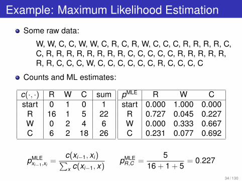
Example: Maximum Likelihood Estimation
Some raw data:
W, W, C, C, W, W, C, R, C, R, W, C, C, C, R, R, R, R, C,
C, R, R, R, R, R, R, R, R, C, C, C, C, C, R, R, R, R, R,
R, R, C, C, C, W, C, C, C, C, C, C, R, C, C, C, C
Counts and ML estimates:
c(·, ·) R W C sum
start 0 1 0 1
R 16 1 5 22
W 0 2 4 6
C 6 2 18 26
pMLE
R W C
start 0.000 1.000 0.000
R 0.727 0.045 0.227
W 0.000 0.333 0.667
C 0.231 0.077 0.692
pMLE
xi�1
,xi=
c(xi�1
, xi)Px c(xi�1
, x)pMLE
R,C =5
16 + 1 + 5
= 0.227
34 / 130

Example: Maximum Likelihood Estimation
35 / 130

Example: Maximum Likelihood Estimation
Some raw data:
W, W, C, C, W, W, C, R, C, R, W, C, C, C, R, R, R, R, C,
C, R, R, R, R, R, R, R, R, C, C, C, C, C, R, R, R, R, R,
R, R, C, C, C, W, C, C, C, C, C, C, R, C, C, C, C
Data sampled from MLE Markov model, order 1:
W, W, C, R, R, R, R, R, R, R, R, R, R, R, R, R, R, R, R,
C, C, C, C, C, C, W, W, C, C, C, R, R, R, C, C, W, C, C,
C, C, C, R, R, R, R, R, C, R, R, C, R, R, R, R, R
Data sampled from MLE Markov model, order 0:
C, R, C, R, R, R, R, C, R, R, C, C, R, C, C, R, R, R, R, C,
C, C, R, C, R, W, R, C, C, C, W, C, R, C, C, W, C, C, C,
C, R, R, C, C, C, R, C, R, R, C, R, C, R, W, R
36 / 130

Recap: Non-Hidden Markov Models
Use states to encode limited amount of information . . .
About the past.
Current state is known given observations.
Log likelihood just depends on pair counts.
L(xN1
) =X
xi�1
,xi
c(xi�1
, xi) log pxi�1
,xi
MLE: count and normalize.
pMLE
xi�1
,xi=
c(xi�1
, xi)Px c(xi�1
, x)
Easy beezy.
37 / 130

Part II
Discrete Hidden Markov Models
38 / 130

Case Study: Austin Weather 2.0
Ignore rain; one sample every two weeks:
C, W, C, C, C, C, W, C, C, C, C, C, C, W, W, C, W, C, W,
W, C, W, C, W, C, C, C, C, C, C, C, C, C, C, C, C, C, C,
W, C, C, C, W, W, C, C, W, W, C, W, C, W, C, C, C, C, C,
C, C, C, C, C, C, C, C, W, C, W, C, C, W, W, C, W, W, W,
C, W, C, C, C, C, C, C, C, C, C, C, W, C, W, W, W, C, C,
C, C, C, W, C, C, W, C, C, C, C, C, C, C, C, C, C, C, W
Does system have state/memory?
39 / 130

Another View
C W C C C C W C C C C C C W W C W C W W C W C W C C
C C C C C C C C C C C C W C C C W W C C W W C W C W
C C C C C C C C C C C C C W C W C C W W C W W W C W
C C C C C C C C C C W C W W W C C C C C W C C W C C
C C C C C C C C C W C C W W C W C C C W C W C W C C
C C C C C C W C C C C C W C C C W C W C W C C W C W
C C C C C C C C C C C C C W C C C W W C C C W C W C
Does system have memory?
How many states?
40 / 130
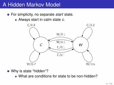
A Hidden Markov Model
For simplicity, no separate start state.
Always start in calm state c.
Why is state “hidden”?
What are conditions for state to be non-hidden?
41 / 130

Contrast: Non-Hidden Markov Models
42 / 130
Why Hidden State?
No “simple” way to determine state given observed.
If see “W ”, doesn’t mean windy season started.
Speech recognition: one HMM per word.
Each state represents different sound in word.
How to tell from observed when state switches?
Hidden models can model same stuff as non-hidden . . .
Using much fewer states.
Pop quiz: name a hidden model with no memory.
43 / 130

The Problem With Hidden State
For observed x = x1
, . . . , xN , what is hidden state h?
Corresponding state sequence h = h1
, . . . , hN+1
.
In non-hidden model, how many h possible given x?
In hidden model, what h are possible given x?
This makes everything difficult.
44 / 130

Three Key Tasks for HMM’s
1
Find single best path in HMM given observed x.
e.g., when did windy season begin?
e.g., when did each sound in word begin?
2
Find total likelihood P(x) of observed.
e.g., to pick which word assigns highest likelihood.
3
Find ML estimates for parameters of HMM.
i.e., estimate arc probabilities to match training data.
45 / 130

Where Are We?
1
Computing the Best Path
2
Computing the Likelihood of Observations
3
Estimating Model Parameters
4
Discussion
46 / 130

What We Want to Compute
Given observed, e.g., x = C, W, C, C, W, . . .
Find state sequence h
⇤with highest likelihood.
h
⇤ = arg max
h
P(h, x)
Why is this easy for non-hidden model?
Given state sequence h, how to compute P(h, x)?
Same as for non-hidden model.
Multiply all arc probabilities along path.
47 / 130

Likelihood of Single State Sequence
Some data: x = W, C, C.
A state sequence: h = c, c, c, w .
Likelihood of path:
P(h, x) = 0.2⇥ 0.6⇥ 0.1 = 0.012
48 / 130

What We Want to Compute
Given observed, e.g., x = C, W, C, C, W, . . .
Find state sequence h
⇤with highest likelihood.
h
⇤ = arg max
h
P(h, x)
Let’s start with simpler problem:
Find likelihood of best state sequence Pbest
(x).Worry about identity of best sequence later.
Pbest
(x) = max
h
P(h, x)
49 / 130

What’s the Problem?
Pbest
(x) = max
h
P(h, x)
For observation sequence of length N . . .
How many different possible state sequences h?
How in blazes can we do max . . .
Over exponential number of state sequences?
50 / 130

Dynamic Programming
Let S0
be start state; e.g., the calm season c.
Let P(S, t) be set of paths of length t . . .
Starting at start state S0
and ending at S . . .
Consistent with observed x1
, . . . , xt .
Any path p 2 P(S, t) must be composed of . . .
Path of length t � 1 to predecessor state S0 ! S . . .
Followed by arc from S0to S labeled with xt .
This decomposition is unique.
P(S, t) =[
S0 xt!S
P(S0, t � 1) · (S0 xt! S)
51 / 130

Dynamic Programming
P(S, t) =[
S0 xt!S
P(S0, t � 1) · (S0 xt! S)
Let ↵̂(S, t) = likelihood of best path of length t . . .
Starting at start state S0
and ending at S.
P(p) = prob of path p = product of arc probs.
↵̂(S, t) = max
p2P(S,t)P(p)
= max
p02P(S0,t�1),S0 xt!SP(p0 · (S0 xt! S))
= max
S0 xt!SP(S0 xt! S) max
p02P(S0,t�1)P(p0)
= max
S0 xt!SP(S0 xt! S)⇥ ↵̂(S0, t � 1)
52 / 130

What Were We Computing Again?
Assume observed x of length T .
Want likelihood of best path of length T . . .
Starting at start state S0
and ending anywhere.
Pbest
(x) = max
h
P(h, x) = max
S↵̂(S, T )
If can compute ↵̂(S, T ), we are done.
If know ↵̂(S, t � 1) for all S, easy to compute ↵̂(S, t):
↵̂(S, t) = max
S0 xt!SP(S0 xt! S)⇥ ↵̂(S0, t � 1)
This looks promising . . .
53 / 130

The Viterbi Algorithm
↵̂(S, 0) = 1 for S = S0
, 0 otherwise.
For t = 1, . . . , T :
For each state S:
↵̂(S, t) = max
S0 xt!SP(S0 xt! S)⇥ ↵̂(S0, t � 1)
The end.
Pbest
(x) = max
h
P(h, x) = max
S↵̂(S, T )
54 / 130

Viterbi and Shortest Path
Equivalent to shortest path problem.
1 23
4
19
1
3
3
10
11
One “state” for each state/time pair (S, t).Iterate through “states” in topological order:
All arcs go forward in time.
If order “states” by time, valid ordering.
d(S) = min
S0!S{d(S0) + distance(S0, S)}
↵̂(S, t) = max
S0 xt!SP(S0 xt! S)⇥ ↵̂(S0, t � 1)
55 / 130

Identifying the Best Path
Wait! We can calc likelihood of best path:
Pbest
(x) = max
h
P(h, x)
What we really wanted: identity of best path.
i.e., the best state sequence h.
Basic idea: for each S, t . . .
Record identity Sprev
(S, t) of previous state S0. . .
In best path of length t ending at state S.
Find best final state.
Backtrace best previous states until reach start state.
56 / 130

The Viterbi Algorithm With Backtrace
↵̂(S, 0) = 1 for S = S0
, 0 otherwise.
For t = 1, . . . , T :
For each state S:
↵̂(S, t) = max
S0 xt!SP(S0 xt! S)⇥ ↵̂(S0, t � 1)
Sprev
(S, t) = arg max
S0 xt!S
P(S0 xt! S)⇥ ↵̂(S0, t � 1)
The end.
Pbest
(x) = max
S↵̂(S, T )
Sfinal
(x) = arg max
S↵̂(S, T )
57 / 130

The Backtrace
Scur
Sfinal
(x)
for t in T , . . . , 1:
Scur
Sprev
(Scur
, t)The best state sequence is . . .
List of states traversed in reverse order.
58 / 130

Example
Some data: C, C, W, W.
↵̂ 0 1 2 3 4
c 1.000 0.600 0.360 0.072 0.014
w 0.000 0.100 0.060 0.036 0.022
↵̂(c, 2) = max{P(c C! c)⇥ ↵̂(c, 1), P(w C! c)⇥ ↵̂(w , 1)}= max{0.6⇥ 0.6, 0.1⇥ 0.1} = 0.36
59 / 130

Example: The Backtrace
Sprev
0 1 2 3 4
c c c c cw c c c w
h
⇤ = arg max
h
P(h, x) = (c, c, c, w , w)
The data: C, C, W, W.
Calm season switching to windy season.
60 / 130

Recap: The Viterbi Algorithm
Given observed x, . . .
Exponential number of hidden sequences h.
Can find likelihood and identity of best path . . .
Efficiently using dynamic programming.
What is time complexity?
61 / 130

Where Are We?
1
Computing the Best Path
2
Computing the Likelihood of Observations
3
Estimating Model Parameters
4
Discussion
62 / 130

What We Want to Compute
Given observed, e.g., x = C, W, C, C, W, . . .
Find total likelihood P(x).
Need to sum likelihood over all hidden sequences:
P(x) =X
h
P(h, x)
Given state sequence h, how to compute P(h, x)?
Multiply all arc probabilities along path.
Why is this sum easy for non-hidden model?
63 / 130

What’s the Problem?
P(x) =X
h
P(h, x)
For observation sequence of length N . . .
How many different possible state sequences h?
How in blazes can we do sum . . .
Over exponential number of state sequences?
64 / 130

Dynamic Programming
Let P(S, t) be set of paths of length t . . .
Starting at start state S0
and ending at S . . .
Consistent with observed x1
, . . . , xt .
Any path p 2 P(S, t) must be composed of . . .
Path of length t � 1 to predecessor state S0 ! S . . .
Followed by arc from S0to S labeled with xt .
P(S, t) =[
S0 xt!S
P(S0, t � 1) · (S0 xt! S)
65 / 130

Dynamic Programming
P(S, t) =[
S0 xt!S
P(S0, t � 1) · (S0 xt! S)
Let ↵(S, t) = sum of likelihoods of paths of length t . . .
Starting at start state S0
and ending at S.
↵(S, t) =X
p2P(S,t)
P(p)
=X
p02P(S0,t�1),S0 xt!S
P(p0 · (S0 xt! S))
=X
S0 xt!S
P(S0 xt! S)X
p02P(S0,t�1)
P(p0)
=X
S0 xt!S
P(S0 xt! S)⇥ ↵(S0, t � 1)
66 / 130

What Were We Computing Again?
Assume observed x of length T .
Want sum of likelihoods of paths of length T . . .
Starting at start state S0
and ending anywhere.
P(x) =X
h
P(h, x) =X
S
↵(S, T )
If can compute ↵(S, T ), we are done.
If know ↵(S, t � 1) for all S, easy to compute ↵(S, t):
↵(S, t) =X
S0 xt!S
P(S0 xt! S)⇥ ↵(S0, t � 1)
This looks promising . . .
67 / 130

The Forward Algorithm
↵(S, 0) = 1 for S = S0
, 0 otherwise.
For t = 1, . . . , T :
For each state S:
↵(S, t) =X
S0 xt!S
P(S0 xt! S)⇥ ↵(S0, t � 1)
The end.
P(x) =X
h
P(h, x) =X
S
↵(S, T )
68 / 130
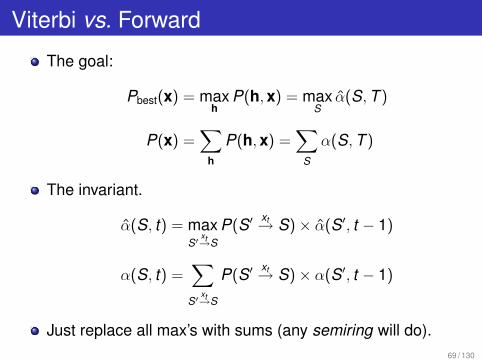
Viterbi vs. Forward
The goal:
Pbest
(x) = max
h
P(h, x) = max
S↵̂(S, T )
P(x) =X
h
P(h, x) =X
S
↵(S, T )
The invariant.
↵̂(S, t) = max
S0 xt!SP(S0 xt! S)⇥ ↵̂(S0, t � 1)
↵(S, t) =X
S0 xt!S
P(S0 xt! S)⇥ ↵(S0, t � 1)
Just replace all max’s with sums (any semiring will do).
69 / 130

Example
Some data: C, C, W, W.
↵ 0 1 2 3 4
c 1.000 0.600 0.370 0.082 0.025
w 0.000 0.100 0.080 0.085 0.059
↵(c, 2) = P(c C! c)⇥ ↵(c, 1) + P(w C! c)⇥ ↵(w , 1)
= 0.6⇥ 0.6 + 0.1⇥ 0.1 = 0.37
70 / 130

Recap: The Forward Algorithm
Can find total likelihood P(x) of observed . . .
Using very similar algorithm to Viterbi algorithm.
Just replace max’s with sums.
Same time complexity.
71 / 130

Where Are We?
1
Computing the Best Path
2
Computing the Likelihood of Observations
3
Estimating Model Parameters
4
Discussion
72 / 130

Training the Parameters of an HMM
Given training data x . . .
Estimate parameters of model . . .
To maximize likelihood of training data.
P(x) =X
h
P(h, x)
73 / 130

What Are The Parameters?
One parameter for each arc:
Identify arc by source S, destination S0, and label x : pS x!S0.
Probs of arcs leaving same state must sum to 1:
X
x ,S0
pS x!S0 = 1 for all S
74 / 130

What Did We Do For Non-Hidden Again?
Likelihood of single path: product of arc probabilities.
Log likelihood can be written as:
L(xN1
) =X
S x!S0
c(S x! S0) log pS x!S0
Just depends on counts c(S x! S0) of each arc.
Each source state corresponds to multinomial . . .
With nonoverlapping parameters.
ML estimation for multinomials: count and normalize!
pMLE
S x!S0 =c(S x! S0)
Px ,S0 c(S x! S0)
75 / 130
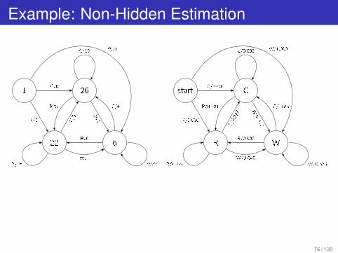
Example: Non-Hidden Estimation
76 / 130

How Do We Train Hidden Models?
Hmmm, I know this one . . .
77 / 130

Review: The EM Algorithm
General way to train parameters in hidden models . . .
To optimize likelihood.
Guaranteed to improve likelihood in each iteration.
Only finds local optimum.
Seeding matters.
78 / 130

The EM Algorithm
Initialize parameter values somehow.
For each iteration . . .
Expectation step: compute posterior (count) of each h.
P̃(h|x) =P(h, x)Ph
P(h, x)
Maximization step: update parameters.
Instead of data x with unknown h, pretend . . .
Non-hidden data where . . .
(Fractional) count of each (h, x) is P̃(h|x).
79 / 130

Applying EM to HMM’s: The E Step
Compute posterior (count) of each h.
P̃(h|x) =P(h, x)Ph
P(h, x)
How to compute prob of single path P(h, x)?
Multiply arc probabilities along path.
How to compute denominator?
This is just total likelihood of observed P(x).
P(x) =X
h
P(h, x)
This looks vaguely familiar.
80 / 130

Applying EM to HMM’s: The M Step
Non-hidden case: single path h with count 1.
Total count of arc is count of arc in h:
c(S x! S0) = ch
(S x! S0)
Normalize.
pMLE
S x!S0 =c(S x! S0)
Px ,S0 c(S x! S0)
Hidden case: every path h has count P̃(h|x).Total count of arc is weighted sum . . .
Of count of arc in each h.
c(S x! S0) =X
h
P̃(h|x)ch
(S x! S0)
Normalize as before.
81 / 130

What’s the Problem?
Need to sum over exponential number of h:
c(S x! S0) =X
h
P̃(h|x)ch
(S x! S0)
If only we had an algorithm for doing this type of thing.
82 / 130

The Game Plan
Decompose sum by time (i.e., position in x).
Find count of each arc at each “time” t .
c(S x! S0) =TX
t=1
c(S x! S0, t) =TX
t=1
X
h2P(S x!S0,t)
P̃(h|x)
P(S x! S0, t) are paths where arc at time t is S x! S0.
P(S x! S0, t) is empty if x 6= xt .
Otherwise, use dynamic programming to compute
c(S xt! S0, t) ⌘X
h2P(Sxt!S0,t)
P̃(h|x)
83 / 130

Let’s Rearrange Some
Recall we can compute P(x) using Forward algorithm:
P̃(h|x) =P(h, x)
P(x)
Some paraphrasing:
c(S xt! S0, t) =X
h2P(Sxt!S0,t)
P̃(h|x)
=1
P(x)
X
h2P(Sxt!S0,t)
P(h, x)
=1
P(x)
X
p2P(Sxt!S0,t)
P(p)
84 / 130

What We Need
Goal: sum over all paths p 2 P(S xt! S0, t).
Arc at time t is S xt! S0.
Let Pi(S, t) be set of (initial) paths of length t . . .
Starting at start state S0
and ending at S . . .
Consistent with observed x1
, . . . , xt .
Let Pf (S, t) be set of (final) paths of length T � t . . .
Starting at state S and ending at any state . . .
Consistent with observed xt+1
, . . . , xT .
Then:
P(S xt! S0, t) = Pi(S, t � 1) · (S xt! S0) · Pf (S0, t)
85 / 130

Translating Path Sets to Probabilities
P(S xt! S0, t) = Pi(S, t � 1) · (S xt! S0) · Pf (S0, t)
Let ↵(S, t) = sum of likelihoods of paths of length t . . .
Starting at start state S0
and ending at S.
Let �(S, t) = sum of likelihoods of paths of length T � t . . .
Starting at state S and ending at any state.
c(S xt! S0, t) =1
P(x)
X
p2P(Sxt!S0,t)
P(p)
=1
P(x)
X
pi2Pi (S,t�1),pf2Pf (S0,t)
P(pi · (Sxt! S0) · pf )
=1
P(x)⇥ p
Sxt!S0
X
pi2Pi (S,t�1)
P(pi)X
pf2Pf (S0,t)
P(pf )
=1
P(x)⇥ p
Sxt!S0 ⇥ ↵(S, t � 1)⇥ �(S0, t)
86 / 130

Mini-Recap
To do ML estimation in M step . . .
Need count of each arc: c(S x! S0).
Decompose count of arc by time:
c(S x! S0) =TX
t=1
c(S x! S0, t)
Can compute count at time efficiently . . .
If have forward probabilities ↵(S, t) . . .
And backward probabilities �(S, T ).
c(S xt! S0, t) =1
P(x)⇥ p
Sxt!S0 ⇥ ↵(S, t � 1)⇥ �(S0, t)
87 / 130

The Forward-Backward Algorithm (1 iter)
Apply Forward algorithm to compute ↵(S, t), P(x).Apply Backward algorithm to compute �(S, t).For each arc S xt! S0
and time t . . .
Compute posterior count of arc at time t if x = xt .
c(S xt! S0, t) =1
P(x)⇥ p
Sxt!S0 ⇥ ↵(S, t � 1)⇥ �(S0, t)
Sum to get total counts for each arc.
c(S x! S0) =TX
t=1
c(S x! S0, t)
For each arc, find ML estimate of parameter:
pMLE
S x!S0 =c(S x! S0)
Px ,S0 c(S x! S0)
88 / 130

The Forward Algorithm
↵(S, 0) = 1 for S = S0
, 0 otherwise.
For t = 1, . . . , T :
For each state S:
↵(S, t) =X
S0 xt!S
pS0 xt!S
⇥ ↵(S0, t � 1)
The end.
P(x) =X
h
P(h, x) =X
S
↵(S, T )
89 / 130
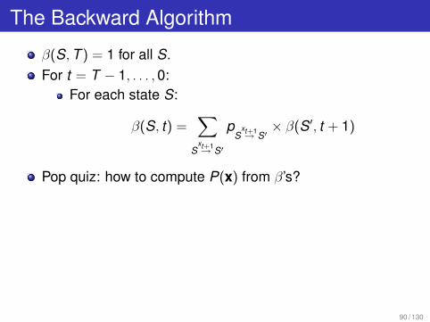
The Backward Algorithm
�(S, T ) = 1 for all S.
For t = T � 1, . . . , 0:
For each state S:
�(S, t) =X
Sxt+1! S0
pS
xt+1! S0⇥ �(S0, t + 1)
Pop quiz: how to compute P(x) from �’s?
90 / 130

Example: The Forward Pass
Some data: C, C, W, W.
↵ 0 1 2 3 4
c 1.000 0.600 0.370 0.082 0.025
w 0.000 0.100 0.080 0.085 0.059
↵(c, 2) = pc C!c⇥ ↵(c, 1) + p
w C!c⇥ ↵(w , 1)
= 0.6⇥ 0.6 + 0.1⇥ 0.1 = 0.37
91 / 130

The Backward Pass
The data: C, C, W, W.
� 0 1 2 3 4
c 0.084 0.123 0.130 0.300 1.000
w 0.033 0.103 0.450 0.700 1.000
�(c, 2) = pc W!c⇥ �(c, 3) + p
c W!w⇥ �(w , 3)
= 0.2⇥ 0.3 + 0.1⇥ 0.7 = 0.13
92 / 130

Computing Arc Posteriors
↵, � 0 1 2 3 4
c 1.000 0.600 0.370 0.082 0.025
w 0.000 0.100 0.080 0.085 0.059
c 0.084 0.123 0.130 0.300 1.000
w 0.033 0.103 0.450 0.700 1.000
c(S x! S0, t) pS x!S0 1 2 3 4
c C! c 0.6 0.878 0.556 0.000 0.000
c W! c 0.2 0.000 0.000 0.264 0.195
c C! w 0.1 0.122 0.321 0.000 0.000
c W! w 0.1 0.000 0.000 0.308 0.098
w C! w 0.2 0.000 0.107 0.000 0.000
w W! w 0.6 0.000 0.000 0.400 0.606
w C! c 0.1 0.000 0.015 0.000 0.000
w W! c 0.1 0.000 0.000 0.029 0.101
93 / 130

Computing Arc Posteriors
↵, � 0 1 2 3 4
c 1.000 0.600 0.370 0.082 0.025
w 0.000 0.100 0.080 0.085 0.059
c 0.084 0.123 0.130 0.300 1.000
w 0.033 0.103 0.450 0.700 1.000
c(S x! S0, t) pS x!S0 1 2 3 4
c C! c 0.6 0.878 0.556 0.000 0.000
c W! c 0.2 0.000 0.000 0.264 0.195
· · · · · · · · · · · · · · · · · ·· · · · · · · · · · · · · · · · · ·
c(c C! c, 2) =1
P(x)⇥ p
c C!c⇥ ↵(c, 1)⇥ �(c, 2)
=1
0.084
⇥ 0.6⇥ 0.600⇥ 0.130 = 0.0556
94 / 130

Summing Arc Counts and Reestimation
1 2 3 4 c(S x! S0) pMLE
S x!S0
c C! c 0.878 0.556 0.000 0.000 1.434 0.523
c W! c 0.000 0.000 0.264 0.195 0.459 0.167
c C! w 0.122 0.321 0.000 0.000 0.444 0.162
c W! w 0.000 0.000 0.308 0.098 0.405 0.148
w C! w 0.000 0.107 0.000 0.000 0.107 0.085
w W! w 0.000 0.000 0.400 0.606 1.006 0.800
w C! c 0.000 0.015 0.000 0.000 0.015 0.012
w W! c 0.000 0.000 0.029 0.101 0.130 0.103
X
x ,S0
c(c x! S0) = 2.742
X
x ,S0
c(w x! S0) = 1.258
95 / 130

Summing Arc Counts and Reestimation
1 2 3 4 c(S x! S0) pMLE
S x!S0
c C! c 0.878 0.556 0.000 0.000 1.434 0.523
c W! c 0.000 0.000 0.264 0.195 0.459 0.167
· · · · · · · · · · · · · · · · · · · · ·· · · · · · · · · · · · · · · · · · · · ·X
x ,S0
c(c x! S0) = 2.742
X
x ,S0
c(w x! S0) = 1.258
c(c C! c) =TX
t=1
c(c C! c, t)
= 0.878 + 0.556 + 0.000 + 0.000 = 1.434
pMLE
c C!c=
c(c C! c)P
x ,S0 c(c x! S0)=
1.434
2.742
= 0.523
96 / 130

Slide for Quiet Contemplation
97 / 130

Another Example
Same initial HMM.
Training data: instead of one sequence, many.
Each sequence is 26 samples, 1 year.
C W C C C C W C C C C C C W W C W C W W C W C W C C
C C C C C C C C C C C C W C C C W W C C W W C W C W
C C C C C C C C C C C C C W C W C C W W C W W W C W
C C C C C C C C C C W C W W W C C C C C W C C W C C
C C C C C C C C C W C C W W C W C C C W C W C W C C
C C C C C C W C C C C C W C C C W C W C W C C W C W
C C C C C C C C C C C C C W C C C W W C C C W C W C
98 / 130

Before and After
99 / 130

Another Starting Point
100 / 130

Recap: The Forward-Backward Algorithm
Also called Baum-Welch algorithm.
Instance of EM algorithm.
Uses dynamic programming to efficiently sum over . . .
Exponential number of hidden state sequences.
Don’t explicitly compute posterior of every h.
Compute posteriors of counts needed in M step.
What is time complexity?
Finds local optimum for parameters in likelihood.
Ending point depends on starting point.
101 / 130

Where Are We?
1
Computing the Best Path
2
Computing the Likelihood of Observations
3
Estimating Model Parameters
4
Discussion
102 / 130

HMM’s and ASR
Old paradigm: DTW.
w⇤ = arg min
w2vocab
distance(A0test
, A0w)
New paradigm: Probabilities.
w⇤ = arg max
w2vocab
P(A0test
|w)
Vector quantization: A0test
) x
test
.
Convert from sequence of 40d feature vectors . . .
To sequence of values from discrete alphabet.
103 / 130

The Basic Idea
For each word w , build HMM modeling P(x|w) = Pw(x).
Training phase.
For each w , pick HMM topology, initial parameters.
Take all instances of w in training data.
Run Forward-Backward on data to update parameters.
Testing: the Forward algorithm.
w⇤ = arg max
w2vocab
Pw(xtest
)
Alignment: the Viterbi algorithm.
When each sound begins and ends.
104 / 130

Recap: Discrete HMM’s
HMM’s are powerful tool for making probabilistic models . . .
Of discrete sequences.
Three key algorithms for HMM’s:
The Viterbi algorithm.
The Forward algorithm.
The Forward-Backward algorithm.
Each algorithm has important role in ASR.
Can do ASR within probabilistic paradigm . . .
Using just discrete HMM’s and vector quantization.
105 / 130

Part III
Continuous Hidden Markov Models
106 / 130

Going from Discrete to Continuous Outputs
What we have: a way to assign likelihoods . . .
To discrete sequences, e.g., C, W, R, C, . . .
What we want: a way to assign likelihoods . . .
To sequences of 40d (or so) feature vectors.
107 / 130

Variants of Discrete HMM’s
Our convention: single output on each arc.
Another convention: output distribution on each arc.
2
4
3
5
2
4
3
5
2
4
3
5
(Another convention: output distribution on each state.)
2
4
3
5
2
4
3
5
108 / 130

Moving to Continuous Outputs
Idea: replace discrete output distribution . . .
With continuous output distribution.
What’s our favorite continuous distribution?
Gaussian mixture models.
109 / 130

Where Are We?
1
The Basics
2
Discussion
110 / 130

Moving to Continuous Outputs
Discrete HMM’s.
Finite vocabulary of outputs.
Each arc labeled with single output x .
Continuous HMM’s.
Finite number of GMM’s: g = 1, . . . , G.
Each arc labeled with single GMM identity g.
111 / 130

What Are The Parameters?
Assume single start state as before.
Old: one parameter for each arc: pS
g!S0.
Identify arc by source S, destination S0, and GMM g.
Probs of arcs leaving same state must sum to 1:
X
g,S0
pS
g!S0 = 1 for all S
New: GMM parameters for g = 1, . . . , G:
pg,j , µg,j , ⌃g,j .
Pg(x) =X
j
pg,j1
(2⇡)d/2|⌃g,j |1/2
e�1
2
(x�µg,j )T ⌃�1
g,j (x�µg,j )
112 / 130

Computing the Likelihood of a Path
Multiply arc and output probabilities along path.
Discrete HMM:
Arc probabilities: pS x!S0.
Output probability 1 if output of arc matches . . .
And 0 otherwise (i.e., path is disallowed).
e.g., consider x = C, C, W, W.
113 / 130

Computing the Likelihood of a Path
Multiply arc and output probabilities along path.
Continuous HMM:
Arc probabilities: pS
g!S0.
Every arc matches any output.
Output probability is GMM probability.
Pg(x) =X
j
pg,j1
(2⇡)d/2|⌃g,j |1/2
e�1
2
(x�µg,j )T ⌃�1
g,j (x�µg,j )
114 / 130

Example: Computing Path Likelihood
Single 1d GMM w/ single component: µ1,1 = 0, �2
1,1 = 1.
Observed: x = 0.3,�0.1; state sequence: h = 1, 1, 2.
P(x) = p1
1!1
⇥ 1p2⇡�
1,1
e�
(0.3�µ1,1)2
2�2
1,1 ⇥
p1
1!2
⇥ 1p2⇡�
1,1
e�
(�0.1�µ1,1)2
2�2
1,1
= 0.7⇥ 0.381⇥ 0.3⇥ 0.397 = 0.0318
115 / 130

The Three Key Algorithms
The main change:
Whenever see arc probability pS x!S0 . . .
Replace with arc probability times output probability:
pS
g!S0 ⇥ Pg(x)
The other change: Forward-Backward.
Need to also reestimate GMM parameters.
116 / 130

Example: The Forward Algorithm
↵(S, 0) = 1 for S = S0
, 0 otherwise.
For t = 1, . . . , T :
For each state S:
↵(S, t) =X
S0 g!S
pS0 g!S
⇥ Pg(xt)⇥ ↵(S0, t � 1)
The end.
P(x) =X
h
P(h, x) =X
S
↵(S, T )
117 / 130

The Forward-Backward Algorithm
Compute posterior count of each arc at time t as before.
c(Sg! S0, t) =
1
P(x)⇥ p
Sg!S0 ⇥Pg(xt)⇥ ↵(S, t � 1)⇥ �(S0, t)
Use to get total counts of each arc as before . . .
c(S x! S0) =TX
t=1
c(S x! S0, t) pMLE
S x!S0 =c(S x! S0)
Px ,S0 c(S x! S0)
But also use to estimate GMM parameters.
Send c(Sg! S0, t) counts for point xt . . .
To estimate GMM g.
118 / 130

An Example, Please?
No more examples for you!
119 / 130

Where Are We?
1
The Basics
2
Discussion
120 / 130
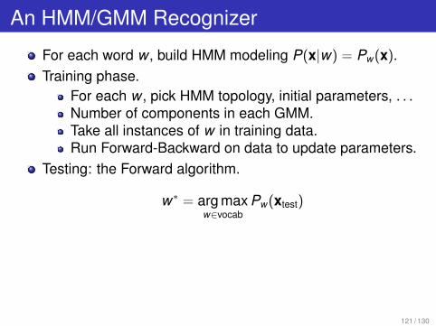
An HMM/GMM Recognizer
For each word w , build HMM modeling P(x|w) = Pw(x).
Training phase.
For each w , pick HMM topology, initial parameters, . . .
Number of components in each GMM.
Take all instances of w in training data.
Run Forward-Backward on data to update parameters.
Testing: the Forward algorithm.
w⇤ = arg max
w2vocab
Pw(xtest
)
121 / 130
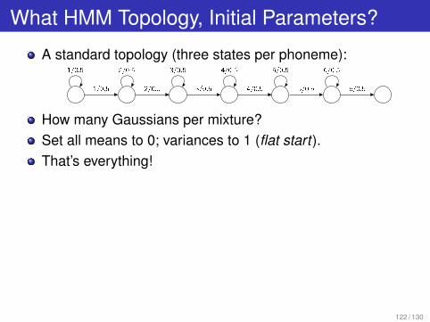
What HMM Topology, Initial Parameters?
A standard topology (three states per phoneme):
How many Gaussians per mixture?
Set all means to 0; variances to 1 (flat start).That’s everything!
122 / 130

HMM/GMM vs. DTW
Old paradigm: DTW.
w⇤ = arg min
w2vocab
distance(A0test
, A0w)
New paradigm: Probabilities.
w⇤ = arg max
w2vocab
P(A0test
|w)
In fact, can design HMM such that
distance(A0test
, A0w) ⇡ � log P(A0
test
|w)
See Holmes, Sec. 9.13, p. 155.
123 / 130

The More Things Change . . .
DTW HMM
template HMM
frame in template state in HMM
DTW alignment HMM path
local path cost transition (log)prob
frame distance output (log)prob
DTW search Viterbi algorithm
124 / 130

What Have We Gained?
Principles!
Probability theory; maximum likelihood estimation.
Can choose path scores and parameter values . . .
In non-arbitrary manner.
Less ways to screw up!
Scalability.
Can extend HMM/GMM framework to . . .
Lots of data; continuous speech; large vocab; etc.
Generalization.
HMM can assign high prob to sample . . .
Even if sample not close to any one training example.
125 / 130

The Markov Assumption
Everything need to know about past . . .
Is encoded in identity of state.
i.e., conditional independence of future and past.
What information do we encode in state?
What information don’t we encode in state?
Issue: the more states, the more parameters.
e.g., the weather.
Solutions.
More states.
Condition on more stuff, e.g., graphical models.
126 / 130

Recap: HMM’s
Together with GMM’s, good way to model likelihood . . .
Of sequences of 40d acoustic feature vectors.
Use state to capture information about past.
Lets you model how data evolves over time.
Not nearly as ad hoc as dynamic time warping.
Need three basic algorithms for ASR.
Viterbi, Forward, Forward-Backward.
All three are efficient: dynamic programming.
Know enough to build basic GMM/HMM recognizer.
127 / 130