lecture 4: instrumental variables -...
TRANSCRIPT
ECON 626: Applied Microeconomics
Lecture 4:
Instrumental Variables
Professors: Pamela Jakiela and Owen Ozier
Department of EconomicsUniversity of Maryland, College Park
Wald
When two variables are measured with error,how do we estimate their true relationship?
ECON 626: Applied Microeconomics Lecture 4: Instrumental Variables, Slide 3
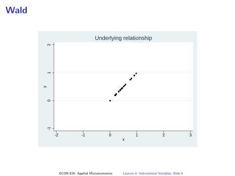
Wald
-10
12
y
-2 -1 0 1 2 3x
Underlying relationship
ECON 626: Applied Microeconomics Lecture 4: Instrumental Variables, Slide 4
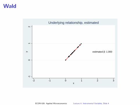
Wald
estimated b: 1.000
-10
12
y
-2 -1 0 1 2 3x
Underlying relationship, estimated
ECON 626: Applied Microeconomics Lecture 4: Instrumental Variables, Slide 4
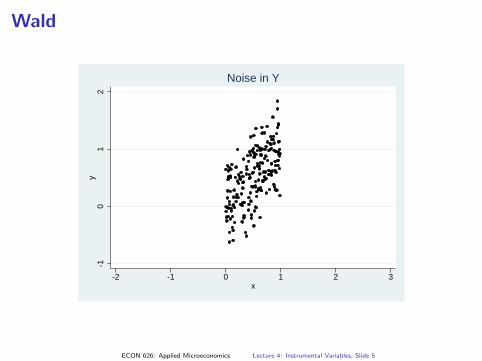
Wald
-10
12
y
-2 -1 0 1 2 3x
Noise in Y
ECON 626: Applied Microeconomics Lecture 4: Instrumental Variables, Slide 5
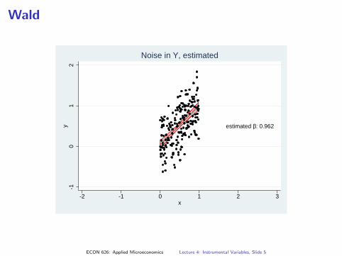
Wald
estimated b: 0.962
-10
12
y
-2 -1 0 1 2 3x
Noise in Y, estimated
ECON 626: Applied Microeconomics Lecture 4: Instrumental Variables, Slide 5
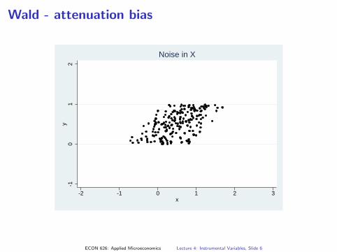
Wald - attenuation bias
-10
12
y
-2 -1 0 1 2 3x
Noise in X
ECON 626: Applied Microeconomics Lecture 4: Instrumental Variables, Slide 6
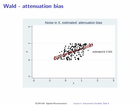
Wald - attenuation bias
estimated b: 0.342
-10
12
y
-2 -1 0 1 2 3x
Noise in X, estimated: attenuation bias
ECON 626: Applied Microeconomics Lecture 4: Instrumental Variables, Slide 6
Wald - attenuation bias
-10
12
y
-2 -1 0 1 2 3x
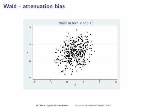
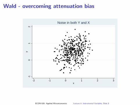
Noise in both Y and X
ECON 626: Applied Microeconomics Lecture 4: Instrumental Variables, Slide 7
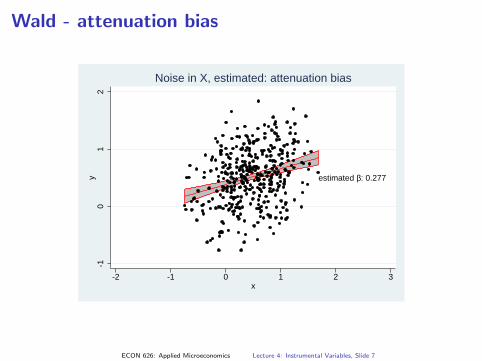
Wald - attenuation bias
estimated b: 0.277
-10
12
y
-2 -1 0 1 2 3x
Noise in X, estimated: attenuation bias
ECON 626: Applied Microeconomics Lecture 4: Instrumental Variables, Slide 7
Wald - attenuation bias
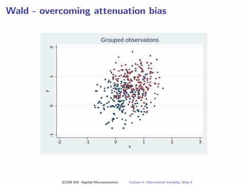
Suppose we have one more piece of information: whether, for eachobservation, the underlying x value (without the measurement error) isabove or below 0.5.
This information will prove to be an “instrument.”
ECON 626: Applied Microeconomics Lecture 4: Instrumental Variables, Slide 8

Wald - attenuation bias
Suppose we have one more piece of information: whether, for eachobservation, the underlying x value (without the measurement error) isabove or below 0.5. This information will prove to be an “instrument.”
ECON 626: Applied Microeconomics Lecture 4: Instrumental Variables, Slide 8
Wald - overcoming attenuation bias
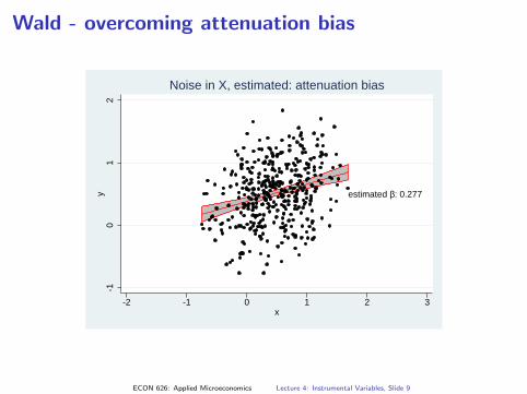
estimated b: 0.277
-10
12
y
-2 -1 0 1 2 3x
Noise in X, estimated: attenuation bias
ECON 626: Applied Microeconomics Lecture 4: Instrumental Variables, Slide 9
Wald - overcoming attenuation bias
-10
12
y
-2 -1 0 1 2 3x
Noise in both Y and X
ECON 626: Applied Microeconomics Lecture 4: Instrumental Variables, Slide 9
Wald - overcoming attenuation bias
-10
12
y
-2 -1 0 1 2 3x
Grouped observations
ECON 626: Applied Microeconomics Lecture 4: Instrumental Variables, Slide 9
Wald - overcoming attenuation bias
-10
12
y
-2 -1 0 1 2 3x
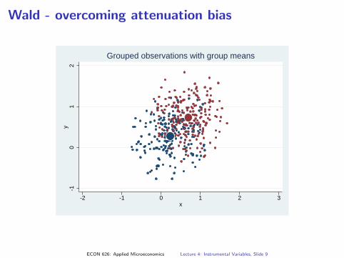
Grouped observations with group means
ECON 626: Applied Microeconomics Lecture 4: Instrumental Variables, Slide 9

Wald - overcoming attenuation bias
estimated b: 0.981
-10
12
y
-2 -1 0 1 2 3x
Grouped observations with Wald estimator
ECON 626: Applied Microeconomics Lecture 4: Instrumental Variables, Slide 9
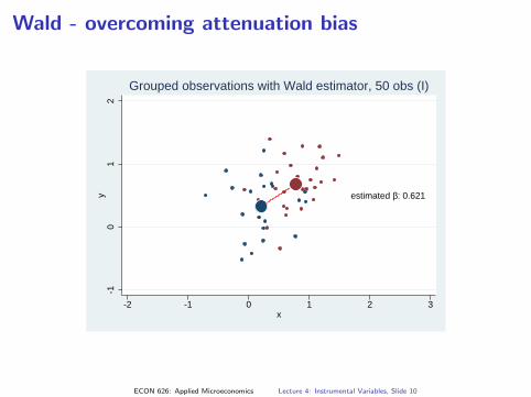
Wald - overcoming attenuation bias
estimated b: 0.621
-10
12
y
-2 -1 0 1 2 3x
Grouped observations with Wald estimator, 50 obs (I)
ECON 626: Applied Microeconomics Lecture 4: Instrumental Variables, Slide 10

Wald - overcoming attenuation bias
estimated b: 2.157
-10
12
y
-2 -1 0 1 2 3x
Grouped observations with Wald estimator, 50 obs (II)
ECON 626: Applied Microeconomics Lecture 4: Instrumental Variables, Slide 11
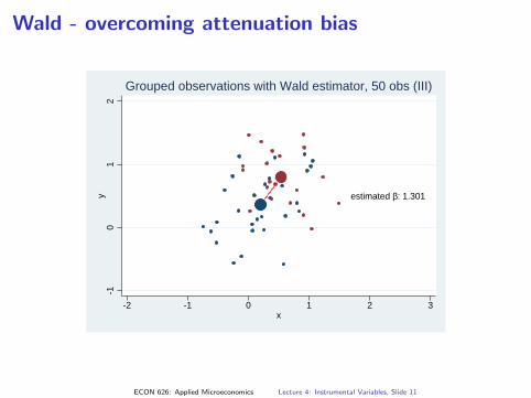
Wald - overcoming attenuation bias
estimated b: 1.301
-10
12
y
-2 -1 0 1 2 3x
Grouped observations with Wald estimator, 50 obs (III)
ECON 626: Applied Microeconomics Lecture 4: Instrumental Variables, Slide 11
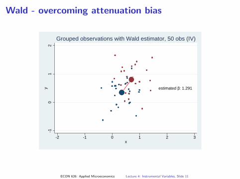
Wald - overcoming attenuation bias
estimated b: 1.291
-10
12
y
-2 -1 0 1 2 3x
Grouped observations with Wald estimator, 50 obs (IV)
ECON 626: Applied Microeconomics Lecture 4: Instrumental Variables, Slide 11
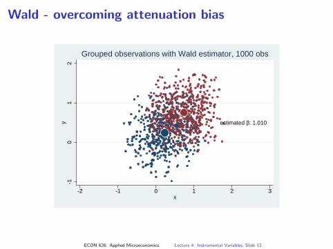
Wald - overcoming attenuation bias
estimated b: 1.010
-10
12
y
-2 -1 0 1 2 3x
Grouped observations with Wald estimator, 1000 obs
ECON 626: Applied Microeconomics Lecture 4: Instrumental Variables, Slide 12

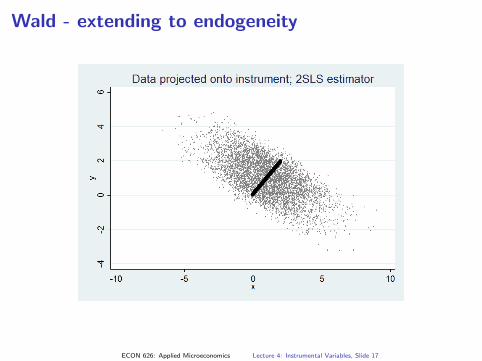
Wald - extending to endogeneity
ECON 626: Applied Microeconomics Lecture 4: Instrumental Variables, Slide 13
Wald - extending to endogeneity
ECON 626: Applied Microeconomics Lecture 4: Instrumental Variables, Slide 13
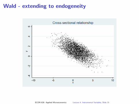
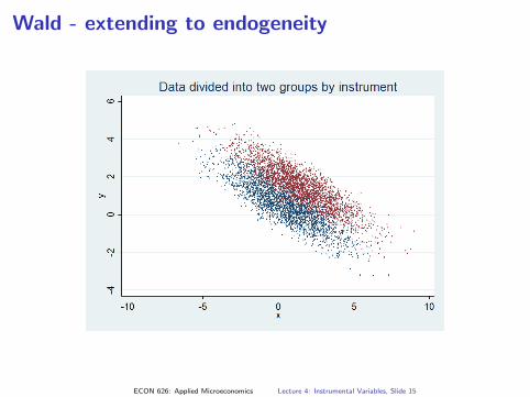
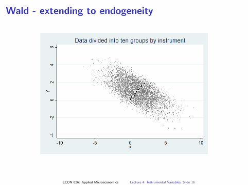
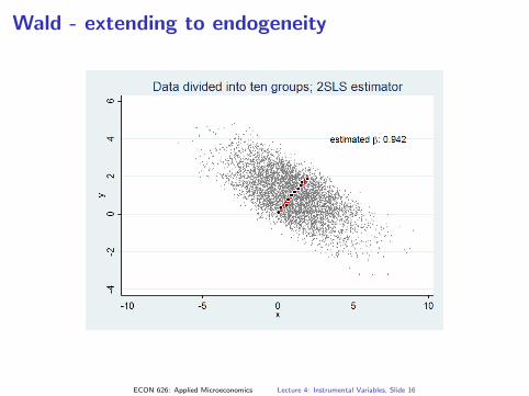
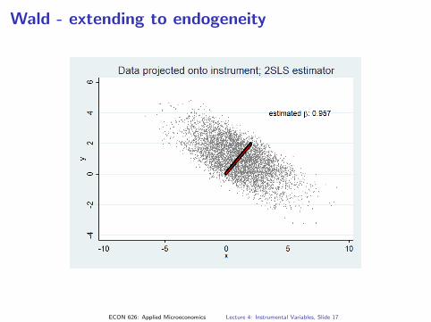
Wald - extending to endogeneity
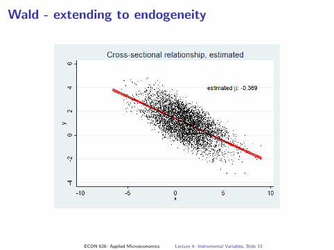
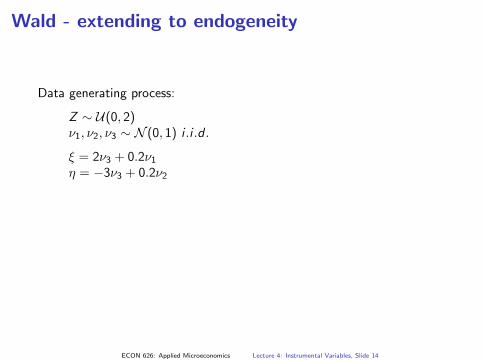
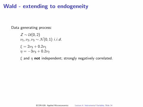
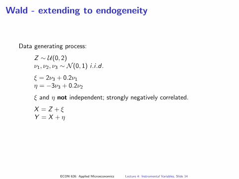
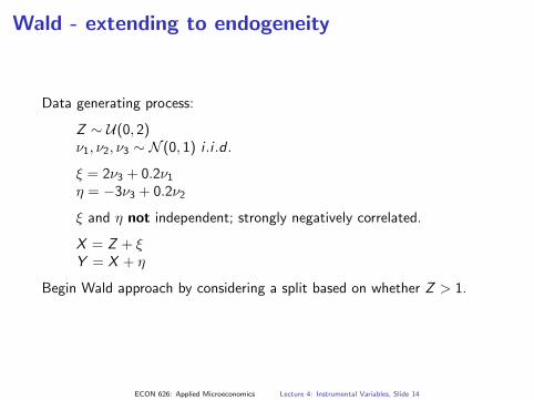
Data generating process:
Z ∼ U(0, 2)ν1, ν2, ν3 ∼ N (0, 1) i .i .d .
ξ = 2ν3 + 0.2ν1η = −3ν3 + 0.2ν2
ξ and η not independent; strongly negatively correlated.
X = Z + ξY = X + η
Begin Wald approach by considering a split based on whether Z > 1.
ECON 626: Applied Microeconomics Lecture 4: Instrumental Variables, Slide 14
Wald - extending to endogeneity
Data generating process:
Z ∼ U(0, 2)ν1, ν2, ν3 ∼ N (0, 1) i .i .d .
ξ = 2ν3 + 0.2ν1η = −3ν3 + 0.2ν2
ξ and η not independent; strongly negatively correlated.
X = Z + ξY = X + η
Begin Wald approach by considering a split based on whether Z > 1.
ECON 626: Applied Microeconomics Lecture 4: Instrumental Variables, Slide 14

Wald - extending to endogeneity
ECON 626: Applied Microeconomics Lecture 4: Instrumental Variables, Slide 15
Wald - extending to endogeneity
ECON 626: Applied Microeconomics Lecture 4: Instrumental Variables, Slide 15
Wald - extending to endogeneity
ECON 626: Applied Microeconomics Lecture 4: Instrumental Variables, Slide 15

Wald - extending to endogeneity
ECON 626: Applied Microeconomics Lecture 4: Instrumental Variables, Slide 15

Wald - extending to endogeneity
ECON 626: Applied Microeconomics Lecture 4: Instrumental Variables, Slide 15
Wald - extending to endogeneity
ECON 626: Applied Microeconomics Lecture 4: Instrumental Variables, Slide 16
Wald - extending to endogeneity
ECON 626: Applied Microeconomics Lecture 4: Instrumental Variables, Slide 16
Wald - extending to endogeneity
ECON 626: Applied Microeconomics Lecture 4: Instrumental Variables, Slide 17
Wald - extending to endogeneity
ECON 626: Applied Microeconomics Lecture 4: Instrumental Variables, Slide 17
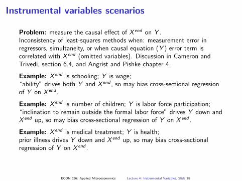
Instrumental variables scenarios
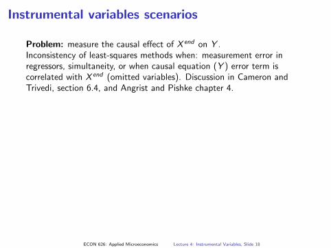
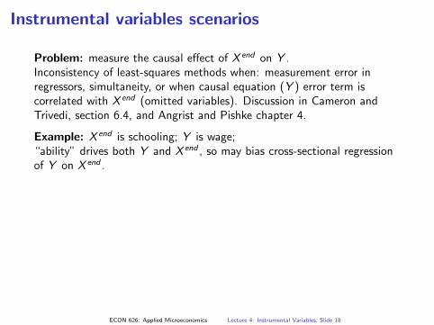
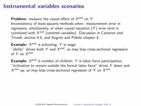
Problem: measure the causal effect of X end on Y .Inconsistency of least-squares methods when: measurement error inregressors, simultaneity, or when causal equation (Y ) error term iscorrelated with X end (omitted variables). Discussion in Cameron andTrivedi, section 6.4, and Angrist and Pishke chapter 4.
Example: X end is schooling; Y is wage;“ability” drives both Y and X end , so may bias cross-sectional regressionof Y on X end .
Example: X end is number of children; Y is labor force participation;“inclination to remain outside the formal labor force” drives Y down andX end up, so may bias cross-sectional regression of Y on X end .
Example: X end is medical treatment; Y is health;prior illness drives Y down and X end up, so may bias cross-sectionalregression of Y on X end .
ECON 626: Applied Microeconomics Lecture 4: Instrumental Variables, Slide 18
Instrumental variables scenarios
Problem: measure the causal casual effect of X end on Y .
Inconsistency of least-squares methods when: measurement error inregressors, simultaneity, or when causal equation (Y ) error term iscorrelated with X end (omitted variables). Discussion in Cameron andTrivedi, section 6.4, and Angrist and Pishke chapter 4.
Example: X end is schooling; Y is wage;“ability” drives both Y and X end , so may bias cross-sectional regressionof Y on X end .
Example: X end is number of children; Y is labor force participation;“inclination to remain outside the formal labor force” drives Y down andX end up, so may bias cross-sectional regression of Y on X end .
Example: X end is medical treatment; Y is health;prior illness drives Y down and X end up, so may bias cross-sectionalregression of Y on X end .
ECON 626: Applied Microeconomics Lecture 4: Instrumental Variables, Slide 18
Instrumental variables scenarios
Problem: measure the causal effect of X end on Y .
Inconsistency of least-squares methods when: measurement error inregressors, simultaneity, or when causal equation (Y ) error term iscorrelated with X end (omitted variables). Discussion in Cameron andTrivedi, section 6.4, and Angrist and Pishke chapter 4.
Example: X end is schooling; Y is wage;“ability” drives both Y and X end , so may bias cross-sectional regressionof Y on X end .
Example: X end is number of children; Y is labor force participation;“inclination to remain outside the formal labor force” drives Y down andX end up, so may bias cross-sectional regression of Y on X end .
Example: X end is medical treatment; Y is health;prior illness drives Y down and X end up, so may bias cross-sectionalregression of Y on X end .
ECON 626: Applied Microeconomics Lecture 4: Instrumental Variables, Slide 18
Instrumental variables scenarios
Problem: measure the causal effect of X end on Y .Inconsistency of least-squares methods when: measurement error inregressors, simultaneity, or when causal equation (Y ) error term iscorrelated with X end (omitted variables). Discussion in Cameron andTrivedi, section 6.4, and Angrist and Pishke chapter 4.
Example: X end is schooling; Y is wage;“ability” drives both Y and X end , so may bias cross-sectional regressionof Y on X end .
Example: X end is number of children; Y is labor force participation;“inclination to remain outside the formal labor force” drives Y down andX end up, so may bias cross-sectional regression of Y on X end .
Example: X end is medical treatment; Y is health;prior illness drives Y down and X end up, so may bias cross-sectionalregression of Y on X end .
ECON 626: Applied Microeconomics Lecture 4: Instrumental Variables, Slide 18
Instrumental variables scenarios
Problem: measure the causal effect of X end on Y .Inconsistency of least-squares methods when: measurement error inregressors, simultaneity, or when causal equation (Y ) error term iscorrelated with X end (omitted variables). Discussion in Cameron andTrivedi, section 6.4, and Angrist and Pishke chapter 4.
Example: X end is schooling; Y is wage;“ability” drives both Y and X end , so may bias cross-sectional regressionof Y on X end .
Example: X end is number of children; Y is labor force participation;“inclination to remain outside the formal labor force” drives Y down andX end up, so may bias cross-sectional regression of Y on X end .
Example: X end is medical treatment; Y is health;prior illness drives Y down and X end up, so may bias cross-sectionalregression of Y on X end .
ECON 626: Applied Microeconomics Lecture 4: Instrumental Variables, Slide 18
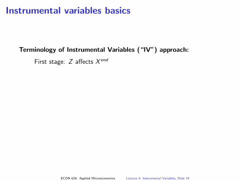
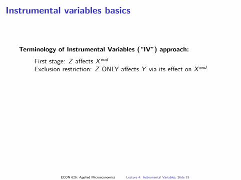
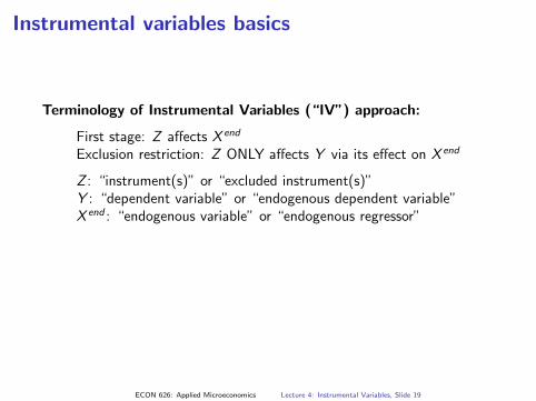
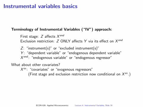
Instrumental variables basics
Terminology of Instrumental Variables (“IV”) approach:
First stage: Z affects X end
Exclusion restriction: Z ONLY affects Y via its effect on X end
Z : “instrument(s)” or “excluded instrument(s)”Y : “dependent variable” or “endogenous dependent variable”X end : “endogenous variable” or “endogenous regressor”
What about other covariates?X ex : “covariates” or “exogenous regressors”
(First stage and exclusion restriction now conditional on X ex .)
ECON 626: Applied Microeconomics Lecture 4: Instrumental Variables, Slide 19

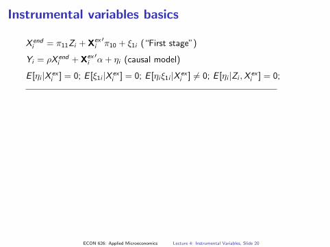
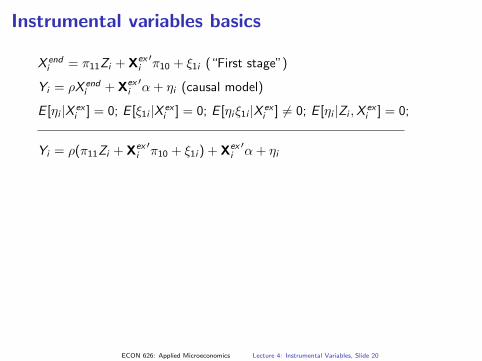
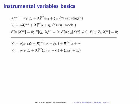
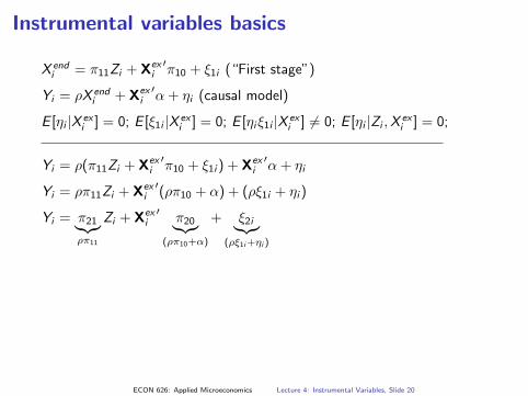
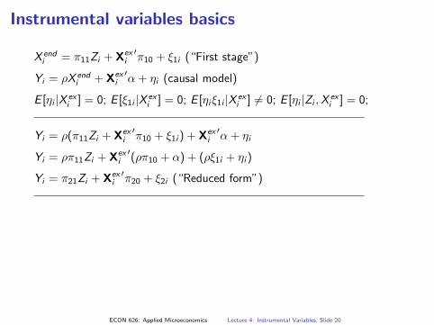
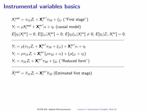
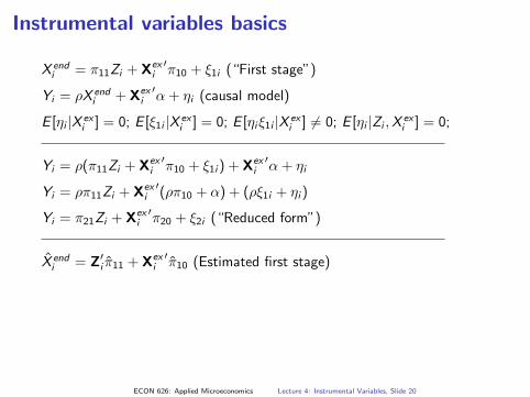
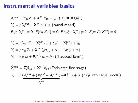
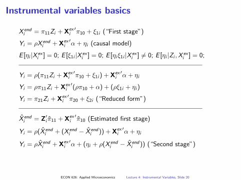
Instrumental variables basics
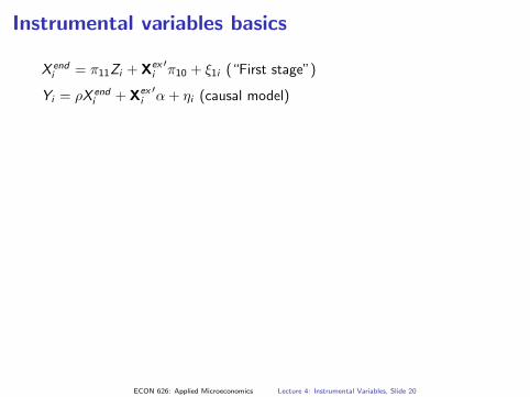
X endi = π11Zi + Xex
i′π10 + ξ1i (“First stage”)
Yi = ρX endi + Xex
i′α + ηi (causal model)
E [ηi |X exi ] = 0; E [ξ1i |X ex
i ] = 0; E [ηiξ1i |X exi ] 6= 0; E [ηi |Zi ,X
exi ] = 0;
Yi = ρ(π11Zi + Xexi
′π10 + ξ1i ) + Xex
i′α + ηi
Yi = ρπ11Zi + Xexi
′(ρπ10 + α) + (ρξ1i + ηi )
Yi = π21︸︷︷︸ρπ11
Zi + Xexi
′π20︸︷︷︸
(ρπ10+α)
+ ξ2i︸︷︷︸(ρξ1i+ηi )
Yi = π21Zi + Xexi
′π20 + ξ2i (“Reduced form”)
X̂ endi = π̂11Zi + Xex
i′π̂10 (Estimated first stage)X̂ end
i = Z′i π̂11 + Xex
i′π̂10 (Estimated first stage)
Yi = ρ (X̂ endi + (X end
i − X̂ endi ))︸ ︷︷ ︸
X endi
+Xexi
′α + ηi (plug into causal model)Yi = ρ(X̂ end
i + (X endi − X̂ end
i )) + Xexi
′α + ηi
Yi = ρX̂ endi + Xex
i′α + (ηi + ρ(X end
i − X̂ endi )) (“Second stage”)
Hence: “Two-stage least squares,” “2SLS” or “TSLS”
ECON 626: Applied Microeconomics Lecture 4: Instrumental Variables, Slide 20
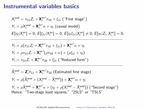
Instrumental variables basics
X endi = π11Zi + Xex
i′π10 + ξ1i (“First stage”)
Yi = ρX endi + Xex
i′α + ηi (causal model)
E [ηi |X exi ] = 0; E [ξ1i |X ex
i ] = 0; E [ηiξ1i |X exi ] 6= 0; E [ηi |Zi ,X
exi ] = 0;
Yi = ρ(π11Zi + Xexi
′π10 + ξ1i ) + Xex
i′α + ηi
Yi = ρπ11Zi + Xexi
′(ρπ10 + α) + (ρξ1i + ηi )
Yi = π21︸︷︷︸ρπ11
Zi + Xexi
′π20︸︷︷︸
(ρπ10+α)
+ ξ2i︸︷︷︸(ρξ1i+ηi )
Yi = π21Zi + Xexi
′π20 + ξ2i (“Reduced form”)
X̂ endi = π̂11Zi + Xex
i′π̂10 (Estimated first stage)X̂ end
i = Z′i π̂11 + Xex
i′π̂10 (Estimated first stage)
Yi = ρ (X̂ endi + (X end
i − X̂ endi ))︸ ︷︷ ︸
X endi
+Xexi
′α + ηi (plug into causal model)Yi = ρ(X̂ end
i + (X endi − X̂ end
i )) + Xexi
′α + ηi
Yi = ρX̂ endi + Xex
i′α + (ηi + ρ(X end
i − X̂ endi )) (“Second stage”)
Hence: “Two-stage least squares,” “2SLS” or “TSLS”
ECON 626: Applied Microeconomics Lecture 4: Instrumental Variables, Slide 20
Instrumental variables basics
X endi = π11Zi + Xex
i′π10 + ξ1i (“First stage”)
Yi = ρX endi + Xex
i′α + ηi (causal model)
E [ηi |X exi ] = 0; E [ξ1i |X ex
i ] = 0; E [ηiξ1i |X exi ] 6= 0; E [ηi |Zi ,X
exi ] = 0;
Yi = ρ(π11Zi + Xexi
′π10 + ξ1i ) + Xex
i′α + ηi
Yi = ρπ11Zi + Xexi
′(ρπ10 + α) + (ρξ1i + ηi )
Yi = π21︸︷︷︸ρπ11
Zi + Xexi
′π20︸︷︷︸
(ρπ10+α)
+ ξ2i︸︷︷︸(ρξ1i+ηi )
Yi = π21Zi + Xexi
′π20 + ξ2i (“Reduced form”)
X̂ endi = π̂11Zi + Xex
i′π̂10 (Estimated first stage)
X̂ endi = Z′
i π̂11 + Xexi
′π̂10 (Estimated first stage)
Yi = ρ (X̂ endi + (X end
i − X̂ endi ))︸ ︷︷ ︸
X endi
+Xexi
′α + ηi (plug into causal model)
Yi = ρ(X̂ endi + (X end
i − X̂ endi )) + Xex
i′α + ηi
Yi = ρX̂ endi + Xex
i′α + (ηi + ρ(X end
i − X̂ endi )) (“Second stage”)
Hence: “Two-stage least squares,” “2SLS” or “TSLS”
ECON 626: Applied Microeconomics Lecture 4: Instrumental Variables, Slide 20
Instrumental variables scenarios
Example: quarter of birth / compulsory schooling instrument
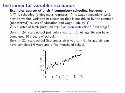
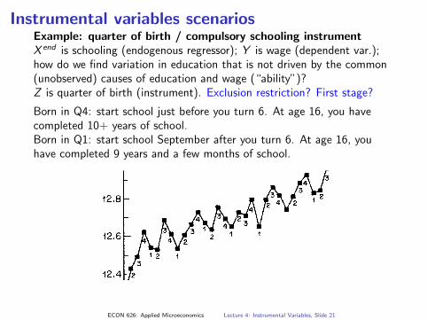
X end is schooling (endogenous regressor); Y is wage (dependent var.);how do we find variation in education that is not driven by the common(unobserved) causes of education and wage (“ability”)?Z is quarter of birth (instrument). Exclusion restriction? First stage?
Born in Q4: start school just before you turn 6. At age 16, you havecompleted 10+ years of school.Born in Q1: start school September after you turn 6. At age 16, youhave completed 9 years and a few months of school.
Finding: wage returns to education via 2SLS slightly larger than OLS.(Angrist and Krueger 1991)
ECON 626: Applied Microeconomics Lecture 4: Instrumental Variables, Slide 21
Instrumental variables scenarios
Example: quarter of birth / compulsory schooling instrumentX end is schooling (endogenous regressor); Y is wage (dependent var.);how do we find variation in education that is not driven by the common(unobserved) causes of education and wage (“ability”)?
Z is quarter of birth (instrument). Exclusion restriction? First stage?
Born in Q4: start school just before you turn 6. At age 16, you havecompleted 10+ years of school.Born in Q1: start school September after you turn 6. At age 16, youhave completed 9 years and a few months of school.
Finding: wage returns to education via 2SLS slightly larger than OLS.(Angrist and Krueger 1991)
ECON 626: Applied Microeconomics Lecture 4: Instrumental Variables, Slide 21
Instrumental variables scenarios
Example: quarter of birth / compulsory schooling instrumentX end is schooling (endogenous regressor); Y is wage (dependent var.);how do we find variation in education that is not driven by the common(unobserved) causes of education and wage (“ability”)?Z is quarter of birth (instrument). Exclusion restriction? First stage?
Born in Q4: start school just before you turn 6. At age 16, you havecompleted 10+ years of school.Born in Q1: start school September after you turn 6. At age 16, youhave completed 9 years and a few months of school.
Finding: wage returns to education via 2SLS slightly larger than OLS.(Angrist and Krueger 1991)
ECON 626: Applied Microeconomics Lecture 4: Instrumental Variables, Slide 21
Instrumental variables scenariosExample: quarter of birth / compulsory schooling instrumentX end is schooling (endogenous regressor); Y is wage (dependent var.);how do we find variation in education that is not driven by the common(unobserved) causes of education and wage (“ability”)?Z is quarter of birth (instrument). Exclusion restriction? First stage?
Born in Q4: start school just before you turn 6. At age 16, you havecompleted 10+ years of school.Born in Q1: start school September after you turn 6. At age 16, youhave completed 9 years and a few months of school.
Finding: wage returns to education via 2SLS slightly larger than OLS.(Angrist and Krueger 1991)
ECON 626: Applied Microeconomics Lecture 4: Instrumental Variables, Slide 21
Instrumental variables scenarios
Example: quarter of birth / compulsory schooling instrumentX end is schooling (endogenous regressor); Y is wage (dependent var.);how do we find variation in education that is not driven by the common(unobserved) causes of education and wage (“ability”)?Z is quarter of birth (instrument). Exclusion restriction? First stage?
Born in Q4: start school just before you turn 6. At age 16, you havecompleted 10+ years of school.Born in Q1: start school September after you turn 6. At age 16, youhave completed 9 years and a few months of school.
Finding: wage returns to education via 2SLS slightly larger than OLS.(Angrist and Krueger 1991)
ECON 626: Applied Microeconomics Lecture 4: Instrumental Variables, Slide 21
Instrumental variables scenarios
Example: same-sex and twins instruments (“human cloning”)
X end is number of children (endogenous regressor);Y is labor force participation (dependent variable);how do we find variation in family size that is not driven by the common(unobserved) causes of family size and labor force participation(“inclination to remain outside the formal labor force”)?Z = two indicators: twins at second birth; first two children same sex(instruments). Exclusion restriction? First stage?
Finding: family size decreases women’s labor force participation, but notby as much as OLS would suggest. (Angrist and Evans 1998, MostlyHarmless Table 4.1.4)
ECON 626: Applied Microeconomics Lecture 4: Instrumental Variables, Slide 22
Instrumental variables scenarios
Example: same-sex and twins instruments
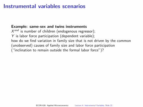
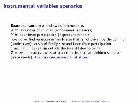
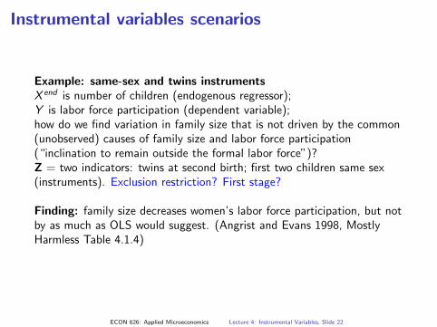
(“human cloning”)
X end is number of children (endogenous regressor);Y is labor force participation (dependent variable);how do we find variation in family size that is not driven by the common(unobserved) causes of family size and labor force participation(“inclination to remain outside the formal labor force”)?
Z = two indicators: twins at second birth; first two children same sex(instruments). Exclusion restriction? First stage?
Finding: family size decreases women’s labor force participation, but notby as much as OLS would suggest. (Angrist and Evans 1998, MostlyHarmless Table 4.1.4)
ECON 626: Applied Microeconomics Lecture 4: Instrumental Variables, Slide 22
Instrumental variables scenarios
Example: same-sex and twins instruments
(“human cloning”)
X end is number of children (endogenous regressor);Y is labor force participation (dependent variable);how do we find variation in family size that is not driven by the common(unobserved) causes of family size and labor force participation(“inclination to remain outside the formal labor force”)?Z = two indicators: twins at second birth; first two children same sex(instruments). Exclusion restriction? First stage?
Finding: family size decreases women’s labor force participation, but notby as much as OLS would suggest. (Angrist and Evans 1998, MostlyHarmless Table 4.1.4)
ECON 626: Applied Microeconomics Lecture 4: Instrumental Variables, Slide 22
Instrumental variables scenarios
Example: same-sex and twins instruments
(“human cloning”)
X end is number of children (endogenous regressor);Y is labor force participation (dependent variable);how do we find variation in family size that is not driven by the common(unobserved) causes of family size and labor force participation(“inclination to remain outside the formal labor force”)?Z = two indicators: twins at second birth; first two children same sex(instruments). Exclusion restriction? First stage?
Finding: family size decreases women’s labor force participation, but notby as much as OLS would suggest. (Angrist and Evans 1998, MostlyHarmless Table 4.1.4)
ECON 626: Applied Microeconomics Lecture 4: Instrumental Variables, Slide 22
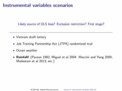
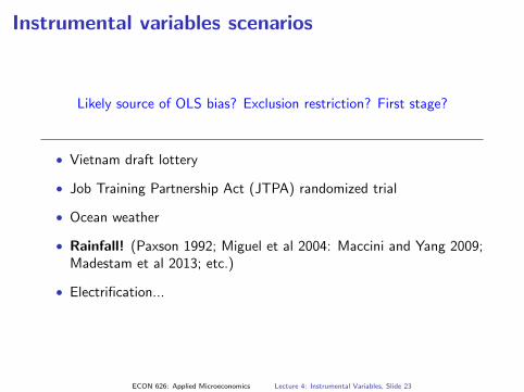
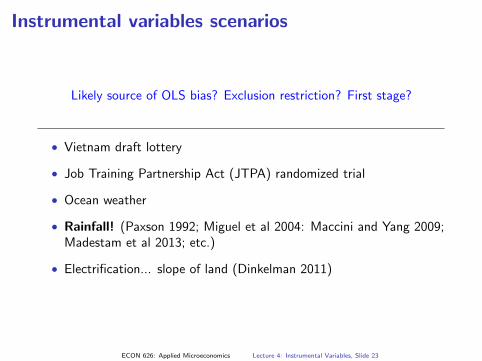
Instrumental variables scenarios
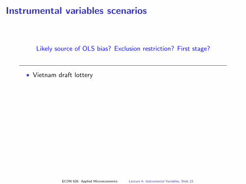
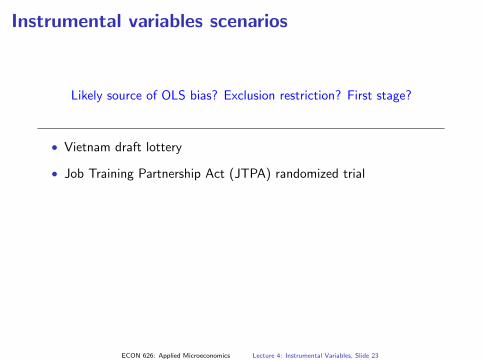
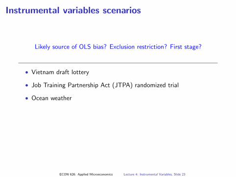
Likely source of OLS bias? Exclusion restriction? First stage?
• Vietnam draft lottery
• Job Training Partnership Act (JTPA) randomized trial
• Ocean weather
• Rainfall! (Paxson 1992; Miguel et al 2004: Maccini and Yang 2009;Madestam et al 2013; etc.)
• Electrification... slope of land (Dinkelman 2011)
ECON 626: Applied Microeconomics Lecture 4: Instrumental Variables, Slide 23
Instrumental variables scenarios
Likely source of OLS bias? Exclusion restriction? First stage?
• Vietnam draft lottery
• Job Training Partnership Act (JTPA) randomized trial
• Ocean weather
• Rainfall! (Paxson 1992; Miguel et al 2004: Maccini and Yang 2009;Madestam et al 2013; etc.)
• Electrification...
slope of land (Dinkelman 2011)
ECON 626: Applied Microeconomics Lecture 4: Instrumental Variables, Slide 23
Instrumental variables scenarios
Likely source of OLS bias? Exclusion restriction? First stage?
• Vietnam draft lottery
• Job Training Partnership Act (JTPA) randomized trial
• Ocean weather
• Rainfall! (Paxson 1992; Miguel et al 2004: Maccini and Yang 2009;Madestam et al 2013; etc.)
• Electrification... slope of land (Dinkelman 2011)
ECON 626: Applied Microeconomics Lecture 4: Instrumental Variables, Slide 23
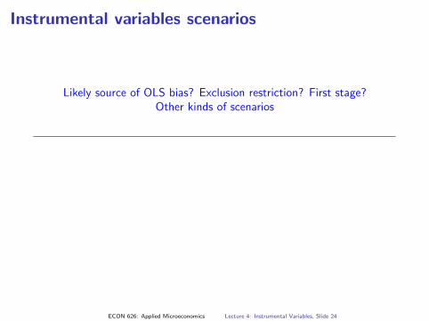
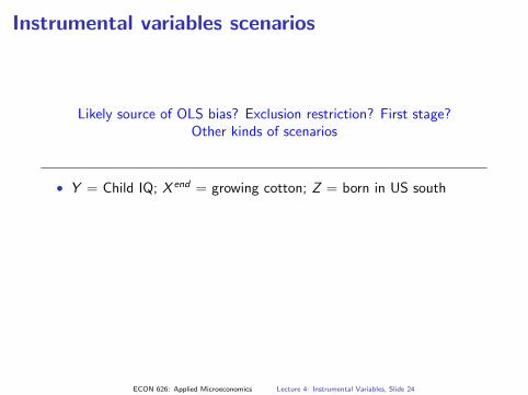
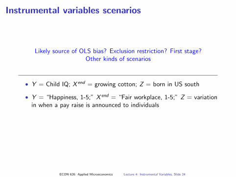
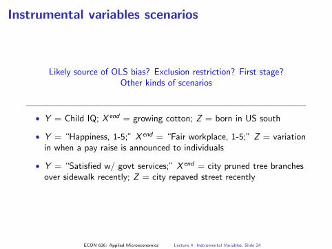
Instrumental variables scenarios
Likely source of OLS bias? Exclusion restriction? First stage?Other kinds of scenarios
• Y = Child IQ; X end = growing cotton; Z = born in US south
• Y = “Happiness, 1-5;” X end = “Fair workplace, 1-5;” Z = variationin when a pay raise is announced to individuals
• Y = “Satisfied w/ govt services;” X end = city pruned tree branchesover sidewalk recently; Z = city repaved street recently
ECON 626: Applied Microeconomics Lecture 4: Instrumental Variables, Slide 24
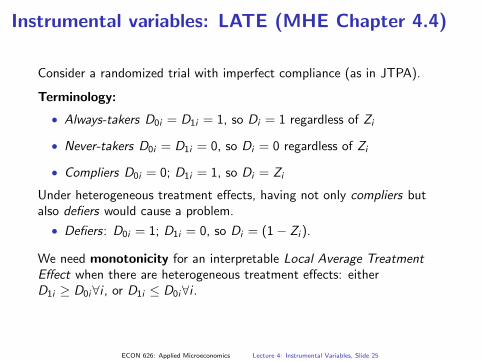
Instrumental variables: LATE (MHE Chapter 4.4)
Consider a randomized trial with imperfect compliance (as in JTPA).
Terminology:
• Always-takers D0i = D1i = 1, so Di = 1 regardless of Zi
• Never-takers D0i = D1i = 0, so Di = 0 regardless of Zi
• Compliers D0i = 0; D1i = 1, so Di = Zi
Under heterogeneous treatment effects, having not only compliers butalso defiers would cause a problem.
• Defiers: D0i = 1; D1i = 0, so Di = (1− Zi ).
We need monotonicity for an interpretable Local Average TreatmentEffect when there are heterogeneous treatment effects: eitherD1i ≥ D0i∀i , or D1i ≤ D0i∀i .
ECON 626: Applied Microeconomics Lecture 4: Instrumental Variables, Slide 25
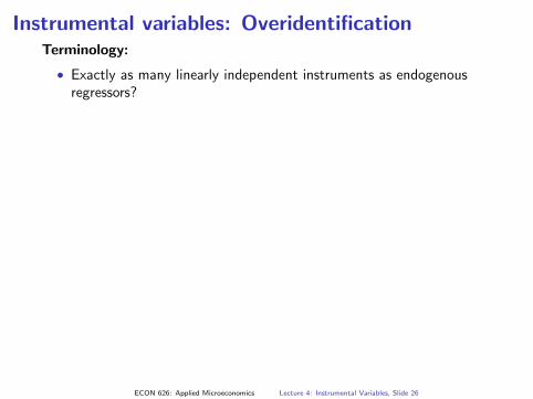
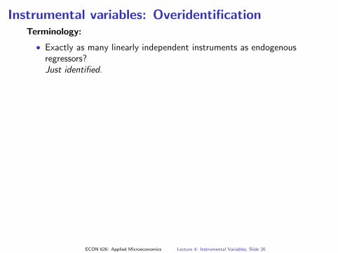
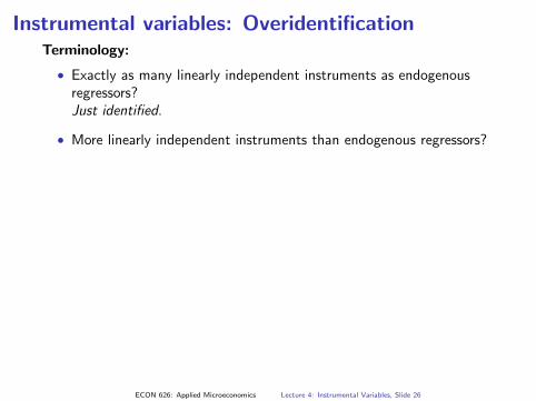
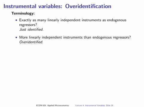
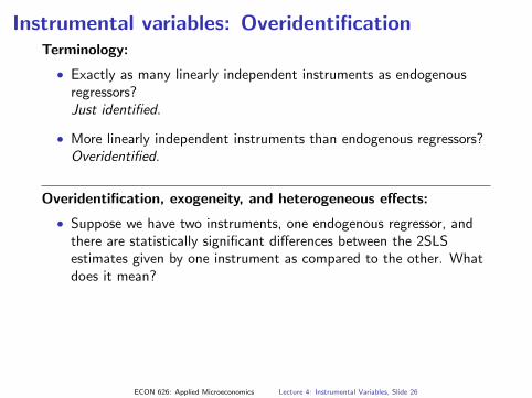
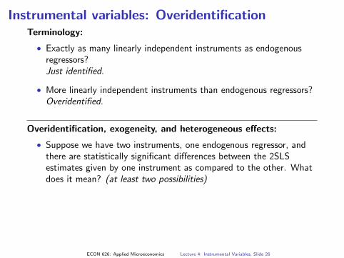
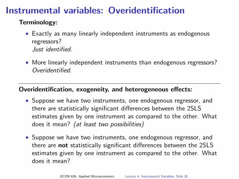
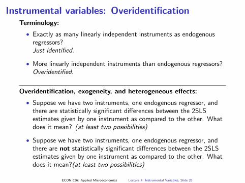
Instrumental variables: OveridentificationTerminology:
• Exactly as many linearly independent instruments as endogenousregressors?
Just identified.
• More linearly independent instruments than endogenous regressors?Overidentified.
Overidentification, exogeneity, and heterogeneous effects:
• Suppose we have two instruments, one endogenous regressor, andthere are statistically significant differences between the 2SLSestimates given by one instrument as compared to the other. Whatdoes it mean? (at least two possibilities)
• Suppose we have two instruments, one endogenous regressor, andthere are not statistically significant differences between the 2SLSestimates given by one instrument as compared to the other. Whatdoes it mean?(at least two possibilities)
ECON 626: Applied Microeconomics Lecture 4: Instrumental Variables, Slide 26
Instrumental variables: OveridentificationTerminology:
• Exactly as many linearly independent instruments as endogenousregressors?Just identified.
• More linearly independent instruments than endogenous regressors?
Overidentified.
Overidentification, exogeneity, and heterogeneous effects:
• Suppose we have two instruments, one endogenous regressor, andthere are statistically significant differences between the 2SLSestimates given by one instrument as compared to the other. Whatdoes it mean? (at least two possibilities)
• Suppose we have two instruments, one endogenous regressor, andthere are not statistically significant differences between the 2SLSestimates given by one instrument as compared to the other. Whatdoes it mean?(at least two possibilities)
ECON 626: Applied Microeconomics Lecture 4: Instrumental Variables, Slide 26
Instrumental variables: OveridentificationTerminology:
• Exactly as many linearly independent instruments as endogenousregressors?Just identified.
• More linearly independent instruments than endogenous regressors?Overidentified.
Overidentification, exogeneity, and heterogeneous effects:
• Suppose we have two instruments, one endogenous regressor, andthere are statistically significant differences between the 2SLSestimates given by one instrument as compared to the other. Whatdoes it mean? (at least two possibilities)
• Suppose we have two instruments, one endogenous regressor, andthere are not statistically significant differences between the 2SLSestimates given by one instrument as compared to the other. Whatdoes it mean?(at least two possibilities)
ECON 626: Applied Microeconomics Lecture 4: Instrumental Variables, Slide 26
Instrumental variables: OveridentificationTerminology:
• Exactly as many linearly independent instruments as endogenousregressors?Just identified.
• More linearly independent instruments than endogenous regressors?Overidentified.
Overidentification, exogeneity, and heterogeneous effects:
• Suppose we have two instruments, one endogenous regressor, andthere are statistically significant differences between the 2SLSestimates given by one instrument as compared to the other. Whatdoes it mean?
(at least two possibilities)
• Suppose we have two instruments, one endogenous regressor, andthere are not statistically significant differences between the 2SLSestimates given by one instrument as compared to the other. Whatdoes it mean?(at least two possibilities)
ECON 626: Applied Microeconomics Lecture 4: Instrumental Variables, Slide 26
Instrumental variables: OveridentificationTerminology:
• Exactly as many linearly independent instruments as endogenousregressors?Just identified.
• More linearly independent instruments than endogenous regressors?Overidentified.
Overidentification, exogeneity, and heterogeneous effects:
• Suppose we have two instruments, one endogenous regressor, andthere are statistically significant differences between the 2SLSestimates given by one instrument as compared to the other. Whatdoes it mean? (at least two possibilities)
• Suppose we have two instruments, one endogenous regressor, andthere are not statistically significant differences between the 2SLSestimates given by one instrument as compared to the other. Whatdoes it mean?(at least two possibilities)
ECON 626: Applied Microeconomics Lecture 4: Instrumental Variables, Slide 26
Instrumental variables: OveridentificationTerminology:
• Exactly as many linearly independent instruments as endogenousregressors?Just identified.
• More linearly independent instruments than endogenous regressors?Overidentified.
Overidentification, exogeneity, and heterogeneous effects:
• Suppose we have two instruments, one endogenous regressor, andthere are statistically significant differences between the 2SLSestimates given by one instrument as compared to the other. Whatdoes it mean? (at least two possibilities)
• Suppose we have two instruments, one endogenous regressor, andthere are not statistically significant differences between the 2SLSestimates given by one instrument as compared to the other. Whatdoes it mean?
(at least two possibilities)
ECON 626: Applied Microeconomics Lecture 4: Instrumental Variables, Slide 26
Instrumental variables: OveridentificationTerminology:
• Exactly as many linearly independent instruments as endogenousregressors?Just identified.
• More linearly independent instruments than endogenous regressors?Overidentified.
Overidentification, exogeneity, and heterogeneous effects:
• Suppose we have two instruments, one endogenous regressor, andthere are statistically significant differences between the 2SLSestimates given by one instrument as compared to the other. Whatdoes it mean? (at least two possibilities)
• Suppose we have two instruments, one endogenous regressor, andthere are not statistically significant differences between the 2SLSestimates given by one instrument as compared to the other. Whatdoes it mean?(at least two possibilities)
ECON 626: Applied Microeconomics Lecture 4: Instrumental Variables, Slide 26
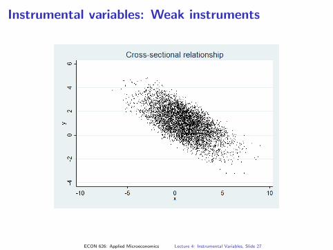
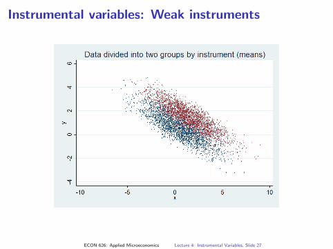
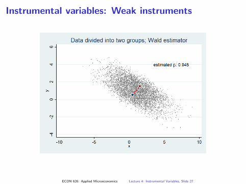
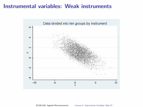
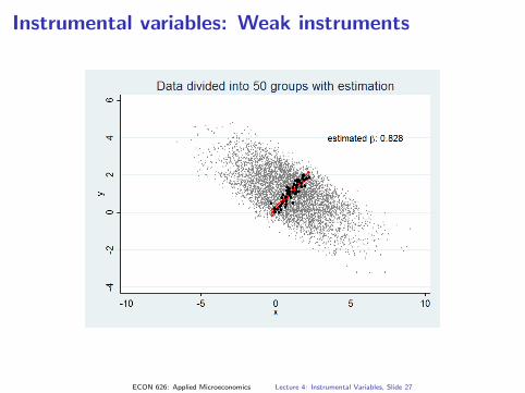
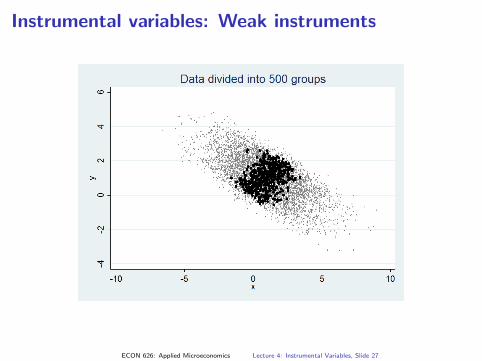
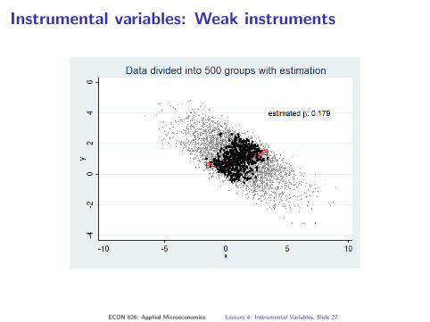
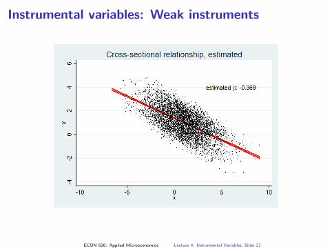
Instrumental variables: Weak instruments
ECON 626: Applied Microeconomics Lecture 4: Instrumental Variables, Slide 27

Instrumental variables: Weak instruments
ECON 626: Applied Microeconomics Lecture 4: Instrumental Variables, Slide 27
Instrumental variables: Weak instruments
ECON 626: Applied Microeconomics Lecture 4: Instrumental Variables, Slide 27
Instrumental variables: Weak instruments
ECON 626: Applied Microeconomics Lecture 4: Instrumental Variables, Slide 27
Instrumental variables: Weak instruments
ECON 626: Applied Microeconomics Lecture 4: Instrumental Variables, Slide 27

Instrumental variables: Weak instruments
ECON 626: Applied Microeconomics Lecture 4: Instrumental Variables, Slide 27

Instrumental variables: Weak instruments
ECON 626: Applied Microeconomics Lecture 4: Instrumental Variables, Slide 27
Instrumental variables: Weak instruments
ECON 626: Applied Microeconomics Lecture 4: Instrumental Variables, Slide 27
Instrumental variables: Weak instruments
ECON 626: Applied Microeconomics Lecture 4: Instrumental Variables, Slide 27
Instrumental variables: Weak instruments
ECON 626: Applied Microeconomics Lecture 4: Instrumental Variables, Slide 27
Instrumental variables: Weak instruments
ECON 626: Applied Microeconomics Lecture 4: Instrumental Variables, Slide 27
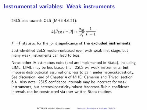
Instrumental variables: Weak instruments
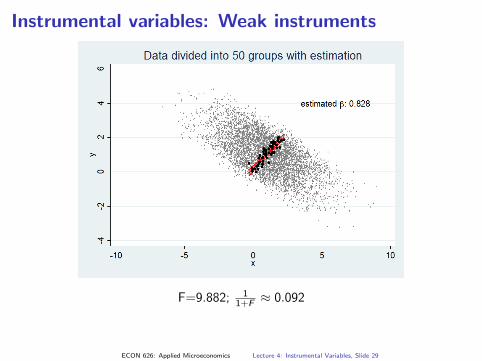
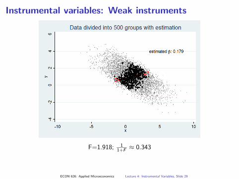
2SLS bias towards OLS (MHE 4.6.21):
E [β̂2SLS − β] ≈ σηξσ2ξ
1
F + 1
F =F statistic for the joint significance of the excluded instruments.
Just-identified 2SLS median-unbiased even with weak first stage, butmany weak instruments can lead to bias.
Note: other IV estimators exist (and are implemented in Stata), includingLIML. LIML may be less biased than 2SLS w/ weak instruments, butimposes distributional assumptions; less to gain under heteroskedasticity.See discussion: end of Chapter 4 of MHE; Cameron and Trivedi section6.4. Also note: 2SLS confidence intervals may be incorrect for weakinstruments, but heteroskedasticity-robust Anderson-Rubin confidenceintervals can be constructed via user-written Stata routines.
ECON 626: Applied Microeconomics Lecture 4: Instrumental Variables, Slide 28
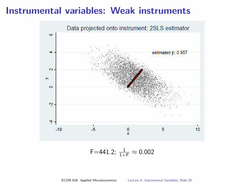
Instrumental variables: Weak instruments
F=441.2; 11+F ≈ 0.002
F=324.3; 11+F ≈ 0.003F=49.07; 11+F ≈ 0.020F=9.882; 11+F ≈ 0.092F=1.918; 11+F ≈ 0.343
F=1.918; 11+F ≈ 0.343
ECON 626: Applied Microeconomics Lecture 4: Instrumental Variables, Slide 29
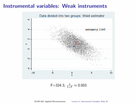
Instrumental variables: Weak instruments
F=441.2; 11+F ≈ 0.002
F=324.3; 11+F ≈ 0.003
F=49.07; 11+F ≈ 0.020F=9.882; 11+F ≈ 0.092F=1.918; 11+F ≈ 0.343
F=1.918; 11+F ≈ 0.343
ECON 626: Applied Microeconomics Lecture 4: Instrumental Variables, Slide 29
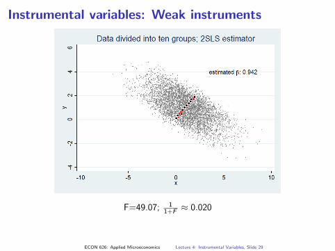
Instrumental variables: Weak instruments
F=441.2; 11+F ≈ 0.002F=324.3; 11+F ≈ 0.003
F=49.07; 11+F ≈ 0.020
F=9.882; 11+F ≈ 0.092F=1.918; 11+F ≈ 0.343
F=1.918; 11+F ≈ 0.343
ECON 626: Applied Microeconomics Lecture 4: Instrumental Variables, Slide 29
Instrumental variables: Weak instruments
F=441.2; 11+F ≈ 0.002F=324.3; 11+F ≈ 0.003F=49.07; 11+F ≈ 0.020
F=9.882; 11+F ≈ 0.092
F=1.918; 11+F ≈ 0.343
F=1.918; 11+F ≈ 0.343
ECON 626: Applied Microeconomics Lecture 4: Instrumental Variables, Slide 29
Instrumental variables: Weak instruments
F=441.2; 11+F ≈ 0.002F=324.3; 11+F ≈ 0.003F=49.07; 11+F ≈ 0.020F=9.882; 11+F ≈ 0.092
F=1.918; 11+F ≈ 0.343
F=1.918; 11+F ≈ 0.343
ECON 626: Applied Microeconomics Lecture 4: Instrumental Variables, Slide 29

Try IV out for yourself.