lecture 4: mobile ad hoc and sensor networks (i)
TRANSCRIPT

Lecture 4: Mobile Ad Hoc and Sensor
Networks (I)
Ing-Ray Chen
CS 6204 Mobile Computing
Virginia Tech
Courtesy of G.G. Richard III for providing some of
the slides
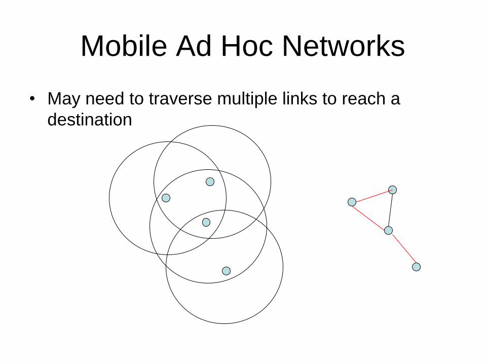
Mobile Ad Hoc Networks
• May need to traverse multiple links to reach a
destination

Mobile Ad Hoc Networks
• Mobility causes route changes

Mobile Ad Hoc Networks
• Formed by wireless hosts which may be mobile
• Don’t need a pre-existing infrastructure – ie, don’t need a backbone network, routers, etc.
• Routes between nodes potentially contain multiple hops
• Why MANET? – Ease, speed of deployment
– Decreased dependence on infrastructure
– Can use in many scenarios where deployment of a wired network is impractical or impossible
– Lots of military applications, but there are others…
,

Many Applications
• Personal area networking – cell phone, laptop, ear phone, wrist watch
• Civilian environments – meeting rooms
– sports stadiums
– groups of boats, small aircraft (wired REALLY impractical!!)
• Emergency operations – search-and-rescue
– policing and fire fighting
• Sensor networks – Groups of sensors embedded in the environment or
scattered over a target area

Many Variations
• Traffic characteristics may differ – Bandwidth/timeliness/reliability requirements
– unicast / broadcast / multicast / geocast
• Symmetric/Asymmetric Capabilities (hetero/homo-geneous)
– transmission ranges and radios may differ
– battery life at different nodes may differ
– processing capacity may be different at different nodes
– speed of movement different
– only some nodes may route packets
– some nodes may act as leaders of nearby nodes (e.g., ―a cluster
head‖)

Challenges
• Limited wireless transmission range
• Broadcast nature of the wireless medium
• Packet losses due to transmission errors
• Rapidly changing topology
• Mobility-induced route changes
• Mobility-induced packet losses
• Battery constraints
• Potentially frequent network partitions
• Ease of snooping on wireless transmissions
• Sensor networks: very resource-constrained!

Hidden Terminal Problem
Nodes A and C cannot hear each other
Transmissions by nodes A and C can collide at node B
On collision, both transmissions are lost
Nodes A and C are hidden from each other
B C A

First Issue: Routing
• Why is Ad hoc Routing Different?
• Host mobility – link failure/repair due to mobility may have
different characteristics than those due to other causes
– traditional routing algorithms assume relatively stable network topology, with few router failures
• Rate of link failure/recovery may be high when nodes move fast
• New performance criteria may be used – route stability despite mobility
– energy consumption (because routers are not connected to power)
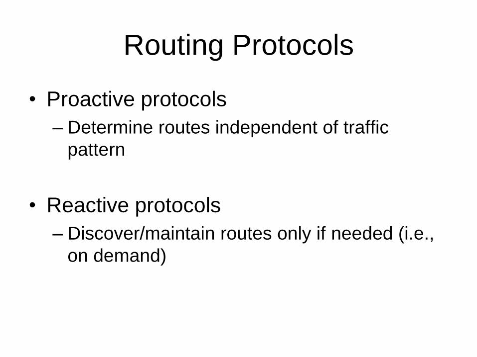
Routing Protocols
• Proactive protocols
– Determine routes independent of traffic
pattern
• Reactive protocols
– Discover/maintain routes only if needed (i.e.,
on demand)

Trade-Off: Proactive vs.
Reactive
• Latency of route discovery – Proactive protocols may have lower latency since routes are
maintained at all times
– Reactive protocols may have higher latency because a route from X to Y will be found only when X attempts to send to Y
• Overhead of route discovery/maintenance – Reactive protocols may have lower overhead since routes
are determined only if needed
– Proactive protocols can (but not necessarily) result in higher overhead due to continuous route updating
• Which approach achieves a better tradeoff depends on the traffic and mobility patterns

Flooding for Data Delivery
• Sender S broadcasts data packet P to all its neighbors
• Each node receiving P forwards P to its neighbors
• Sequence numbers will be used to avoid the possibility of forwarding the same packet more than once
• Packet P reaches destination D provided that D is reachable from sender S
• Node D does not forward the packet

Flooding for Data Delivery
B
A
S E
F
H
J
D
C
G
I
K
Represents that connected nodes are within each
other’s transmission range
Z
Y
Represents a node that has received packet P
M
N
L

Flooding for Data Delivery
B
A
S E
F
H
J
D
C
G
I
K
Represents transmission of packet P
Represents a node that receives packet P for
the first time
Z
Y Broadcast transmission
M
N
L

Flooding for Data Delivery
B
A
S E
F
H
J
D
C
G
I
K
Node H receives packet P from two neighbors:
potential for collision
Z
Y
M
N
L

Flooding for Data Delivery
B
A
S E
F
H
J
D
C
G
I
K
Node C receives packet P from G and H, but does not
forward it again, because node C has already forwarded
packet P once
Z
Y
M
N
L

Flooding for Data Delivery
B
A
S E
F
H
J
D
C
G
I
K
Z
Y
M
Nodes J and K both broadcast packet P to node D
Since nodes J and K are hidden from each other, their
transmissions may collide
=> Packet P may not be delivered to node D after all,
despite the use of flooding!!
N
L

Flooding for Data Delivery
B
A
S E
F
H
J
D
C
G
I
K
Z
Y
• Node D does not forward packet P, because node D
is the intended destination of packet P
M
N
L

Flooding for Data Delivery
B
A
S E
F
H
J
D
C
G
I
K
Flooding completed
Nodes unreachable from S do not receive packet P (e.g., node Z)
Nodes for which all paths from S go through the destination D
also do not receive packet P (example: node N)
Z
Y
M
N
L

Flooding for Data Delivery
B
A
S E
F
H
J
D
C
G
I
K
Flooding may deliver packets to too many nodes
(in the worst case, all nodes reachable from the sender
may receive the packet)
Z
Y
M
N
L

Flooding for Data Delivery: Advantages
• Simplicity
• Potentially more efficient when transmitting small
data packets relatively infrequently and the
overhead of explicit route discovery/maintenance
incurred by other protocols is relatively high
because of topology changes
• Potentially higher reliability of data delivery
– Because of the existence of multiple paths
– For high mobility patterns, it may be the only
reasonable choice

Flooding for Data Delivery: Disadvantages
• high overhead per packet – Flooding is expensive
• Potentially lower reliability of data delivery – Flooding uses broadcasting -- hard to implement
reliable broadcast delivery without significantly increasing overhead
– Broadcasting in IEEE 802.11 MAC is unreliable
– In our example, nodes J and K may transmit to node D simultaneously, resulting in loss of the packet
– in this case, destination would not receive the packet at all

Flooding of Control Packets
• Many protocols perform (potentially limited)
flooding of control packets, instead of data
packets
• The control packets are used to discover
routes
• Discovered routes are subsequently used to
send data packets without flooding
• Overhead of control packet flooding is
amortized over data packets transmitted
between two consecutive control packet floods

Metrics for Ad Hoc Routing
• Want to optimize – Number of hops
– Distance
– Latency
– Load balancing for congested links
– Cost ($$$)
– Route stability
– Energy consumption
• Many existing ad hoc routing descriptions use # of hops
• More work recently on latency, load balancing, etc.

Dynamic Source Routing – DSR
(Ref [11]) • When node S wants to send a packet to node D, but
does not know a route to D, node S initiates a route discovery by flooding a Route Request (RREQ) packet
• Each node appends its identifier when forwarding RREQ
• A route if discovered will return from D to S
• When node S sends a data packet to D, the entire route is included in the packet header – hence the name source routing
• Intermediate nodes use the source route included in a packet to determine to whom a packet should be forwarded
• Reactive: Routes are discovered on demand: only when a node wants to send data and the route to destination is not known

Route Discovery in DSR
B
A
S E
F
H
J
D
C
G
I
K
Z
Y
Represents a node that has received RREQ for D
M
N
L

Route Discovery in DSR
B
A
S E
F
H
J
D
C
G
I
K
Represents transmission of RREQ
Z
Y Broadcast transmission
M
N
L
[S]
[X,Y] Represents list of identifiers appended to RREQ

Route Discovery in DSR
B
A
S E
F
H
J
D
C
G
I
K
Node H receives packet RREQ from two neighbors:
potential for collision
Z
Y
M
N
L
[S,E]
[S,C]
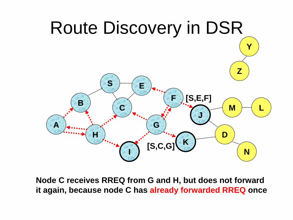
Route Discovery in DSR
B
A
S E
F
H
J
D
C
G
I
K
Node C receives RREQ from G and H, but does not forward
it again, because node C has already forwarded RREQ once
Z
Y
M
N
L
[S,C,G]
[S,E,F]
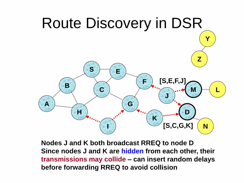
Route Discovery in DSR
B
A
S E
F
H
J
D
C
G
I
K
Z
Y
M
Nodes J and K both broadcast RREQ to node D
Since nodes J and K are hidden from each other, their
transmissions may collide – can insert random delays
before forwarding RREQ to avoid collision
N
L
[S,C,G,K]
[S,E,F,J]

Route Discovery in DSR
B
A
S E
F
H
J
D
C
G
I
K
Z
Y
Node D does not forward RREQ, because node D
is the intended target of the route discovery
M
N
L
[S,E,F,J,M]

Route Discovery in DSR: Part 2
• Destination D, on receiving the first RREQ, sends a Route Reply (RREP)
• RREP is sent on a route obtained by reversing the route of RREQ
• RREP includes the route from D to S on which RREQ was received by node D – Node S on receiving RREP, caches the route
included in the RREP

Route Reply in DSR
B
A
S E
F
H
J
D
C
G
I
K
Z
Y
M
N
L
RREP [S,E,F,J,D]
Represents RREP control message

Data Delivery in DSR
B
A
S E
F
H
J
D
C
G
I
K
Z
Y
M
N
L
DATA [S,E,F,J,D]
Packet header size grows with route length
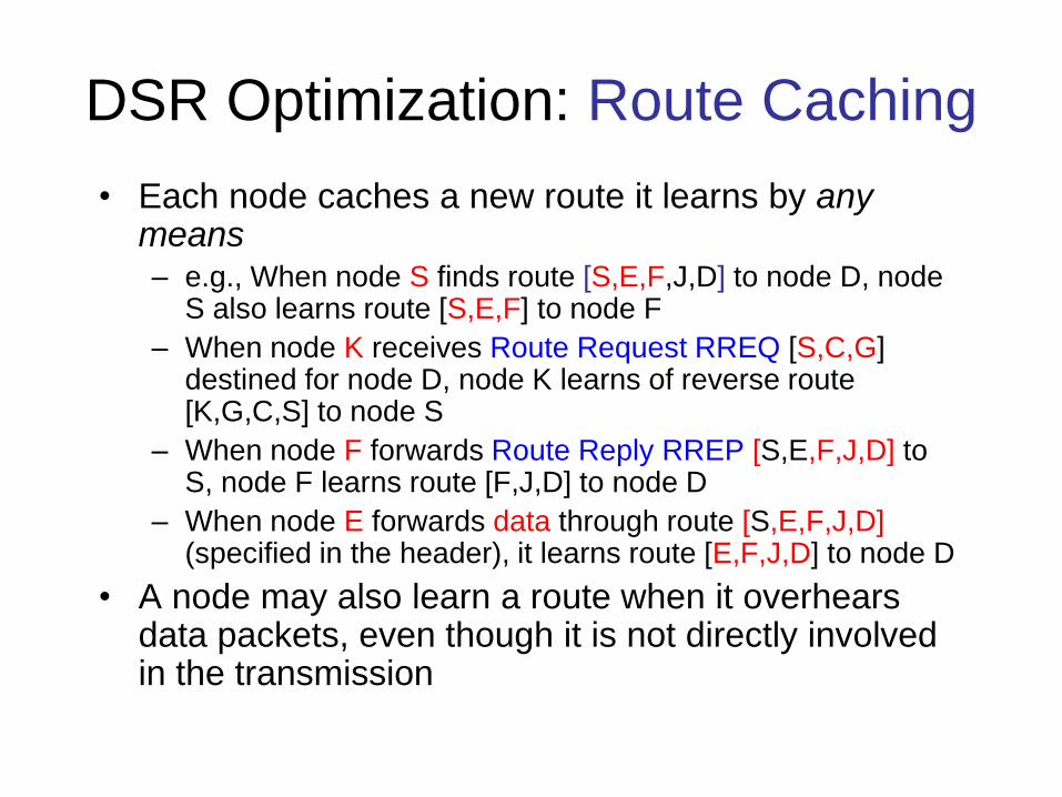
DSR Optimization: Route Caching
• Each node caches a new route it learns by any means – e.g., When node S finds route [S,E,F,J,D] to node D, node
S also learns route [S,E,F] to node F
– When node K receives Route Request RREQ [S,C,G] destined for node D, node K learns of reverse route [K,G,C,S] to node S
– When node F forwards Route Reply RREP [S,E,F,J,D] to S, node F learns route [F,J,D] to node D
– When node E forwards data through route [S,E,F,J,D] (specified in the header), it learns route [E,F,J,D] to node D
• A node may also learn a route when it overhears data packets, even though it is not directly involved in the transmission

Route Caching (2)
• Use of route cache
– can speed up route discovery
– can reduce propagation of route requests
• When node S learns that a route to node D is
broken, it uses another route from its local cache, if
such a route to D exists in its cache.
• Otherwise, node S initiates route discovery by
sending a RREQ packet
• Node X, on receiving a RREQ for some node D, can
send a RREP directly if node X knows a route to
node D

Route Caching (3)
B
A
S E
F
H
J
D
C
G
I
K
[P,Q,R] Represents a cached route in a node
(DSR maintains the cached routes in a tree format)
M
N
L
[S,E,F,J,D] [E,F,J,D]
[C,S]
[G,C,S]
[F,J,D],[F,E,S]
[J,F,E,S]
Z

Route Caching (4)
B
A
S E
F
H
J
D
C
G
I
K
Z
M
N
L
[S,E,F,J,D] [E,F,J,D]
[C,S]
[G,C,S]
[F,J,D],[F,E,S]
[J,F,E,S]
RREQ
When node Z sends a route request
for node C, node K sends back a route
reply [Z,K,G,C] to node Z using a locally cached route
[K,G,C,S] RREP
RREQ

Route Error (RERR)
B
A
S E
F
H
J
D
C
G
I
K
Z
Y
M
N
L
RERR [J-D]
when J attempt to forward the data packet (with route SEFJD) to D
but J-D fails, J sends a route error packet to S along route J-F-E-S
Nodes hearing RERR update their route cache to remove link J-D

Route Caching: Beware!
• Stale caches can adversely affect performance
• With passage of time and host mobility, cached routes may become invalid
• A sender host may try several stale routes (obtained from local cache, or replied from cache by other nodes), before finding a good route
• It may be more expensive to try several broken routes than to simply discover a new one!
• Wireless link is unreliable, so news of broken routes through RERR may not even propagate completely!

DSR Caching: Advantages
• Routes maintained only between nodes who need to communicate – reduces overhead of route maintenance
• Route caching can further reduce route discovery overhead
• A single route discovery may yield many routes to the destination, due to intermediate nodes replying from local caches

DSR Caching: Disadvantages
• An intermediate node may send RREP using a stale
cached route, thus polluting other caches
• This problem can be eased if some mechanism to
purge (potentially) invalid cached routes is incorporated
– Static timeout
– Adaptive timeout of a link based on:
• expected rate of mobility (mobility prediction is useful here)
• observed link usage and breakage
• Contention if many RREP packets come back due to nodes replying using their local cache
– Route Reply Storm problem • Don’t send if overhearing another RREP with a shorter route
Another Reactive Protocol: Ad-Hoc
On-Demand Distance Vector (AODV)
• Same RREQ-RREP-RERR format except that each node maintains a route table
• Significantly more complicated protocol than DSR, because avoiding routing loops is much more difficult
– Loop elimination easy in DSR because the entire route is available!
• The following pictorial does not expose the complexity of AODV—just to give a basic idea

Route Requests in AODV
B
A
S E
F
H
J
D
C
G
I
K
Z
Y
Represents a node that has received RREQ from S for D
M
N
L

Route Requests in AODV
B
A
S E
F
H
J
D
C
G
I
K
Represents transmission of RREQ
Z
Y
M
N
L
RREQ
RREQ
RREQ

Route Requests in AODV
B
A
S E
F
H
J
D
C
G
I
K
Represents links on Reverse Path, recorded by
Intermediate nodes in their route tables
Z
Y
M
N
L

Reverse Path Setup in AODV
B
A
S E
F
H
J
D
C
G
I
K
Node C receives RREQ from G and H, but does not
forward it again, because node C has already
forwarded RREQ once
Z
Y
M
N
L

Reverse Path Setup in AODV
B
A
S E
F
H
J
D
C
G
I
K
Z
Y
M
N
L

Reverse Path Setup in AODV
B
A
S E
F
H
J
D
C
G
I
K
Z
Y
• When D receives RREQ, it unitcasts RREP to S (without
putting down the entire route on the packet).
• Since each node receiving the request caches a route back
to S, the RREP can be unicast back from D to S
M
N
L
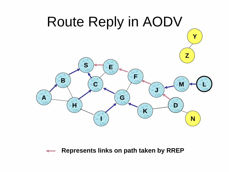
Route Reply in AODV
B
A
S E
F
H
J
D
C
G
I
K
Z
Y
Represents links on path taken by RREP
M
N
L

Forward Path Setup in AODV
B
A
S E
F
H
J
D
C
G
I
K
Z
Y
M
N
L
Forward links are recorded in the routing tables
when RREP travels along the reverse path
Represents a link on the forward path

Data Delivery in AODV
B
A
S E
F
H
J
D
C
G
I
K
Z
Y
M
N
L
Each node uses links stored in the routing table to
forward data packet.
Route is not included in packet header.
DATA

Routing Table Format in AODV
Slide from NIST

Wireless Sensor Networks
• Special case of the general ad hoc networking problem
• Much more resource constrained
• Special-purpose
• May have special restrictions, such as:
– Re-deployment, movement impossible
– Recharge impossible
– Likelihood of many nodes being destroyed, or compromised (through capture)
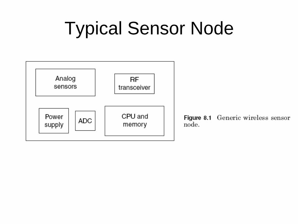
Typical Sensor Node
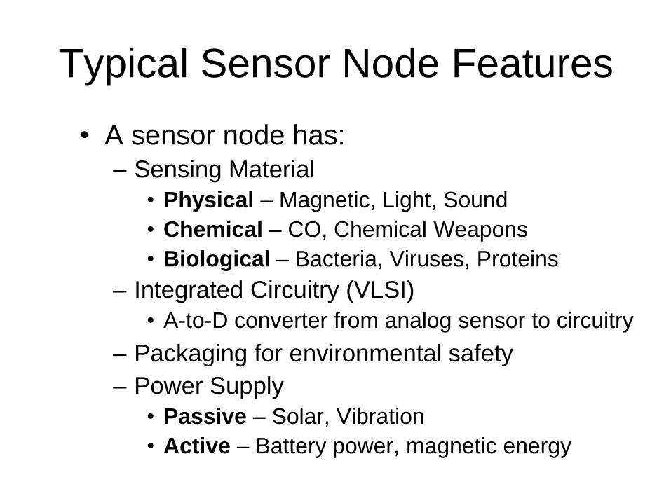
Typical Sensor Node Features
• A sensor node has:
– Sensing Material
• Physical – Magnetic, Light, Sound
• Chemical – CO, Chemical Weapons
• Biological – Bacteria, Viruses, Proteins
– Integrated Circuitry (VLSI)
• A-to-D converter from analog sensor to circuitry
– Packaging for environmental safety
– Power Supply
• Passive – Solar, Vibration
• Active – Battery power, magnetic energy

Advances in Wireless Sensor
Nodes
Consider Multiple Generations of Berkeley Motes
Model Mica Mica-2 Mica-Z Imote2
(Intel)
Date 2002 2003 2004 2007
CPU 4 MHz 7 MHz 7 MHz 14MHz
Flash
Memory 128 KB 128 KB 128 KB 32M
RAM 4 KB 4 KB 4 KB 256KB
Data
rate 40 Kbps 76 Kbps 250 Kbps 250 Kbps

Historical Comparison
Consider a 40 Year Old Computer
Model Honeywell H-300 Mica 2
Date 6/1964 7/2003
CPU 2 MHz 4 MHz
Flash
Memory None 128 KB
RAM 32 KB 4 KB

Smart Home / Smart
Office/Cyber Physical Systems
• Sensors controlling
appliances and
electrical devices in
the house.
• Better lighting and
heating in office
buildings.
• The Pentagon
building has used
sensors extensively.

Military
Remote deployment of sensors for tactical monitoring of enemy troop movements.

Industrial & Commercial
• Numerous industrial and commercial
applications:
– Agricultural Crop Conditions
– Inventory Tracking
– Parts Tracking
– Automated Problem Reporting
– RFID – Theft Deterrent and Customer Tracing
– Plant Equipment Maintenance Monitoring

Traffic Management & Monitoring
• Future cars could use wireless sensors to: – Handle Accidents
– Handle Thefts
Sensors embedded in the roads to:
– Monitor traffic flows
– Provide real-time route updates

Query-based Sensor Networks
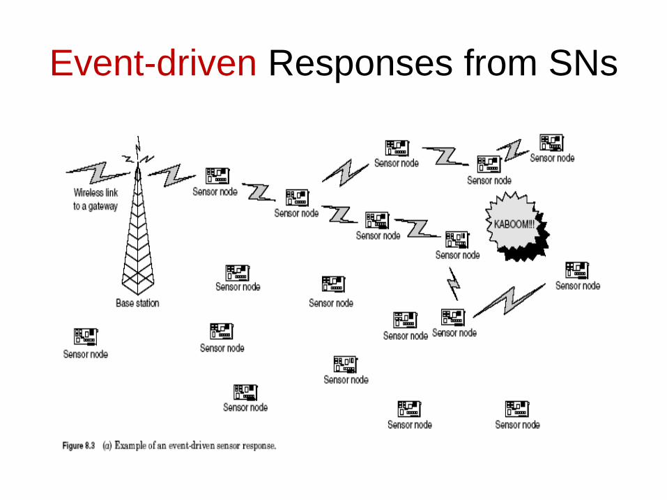
Event-driven Responses from SNs

Periodic Responses from SNs
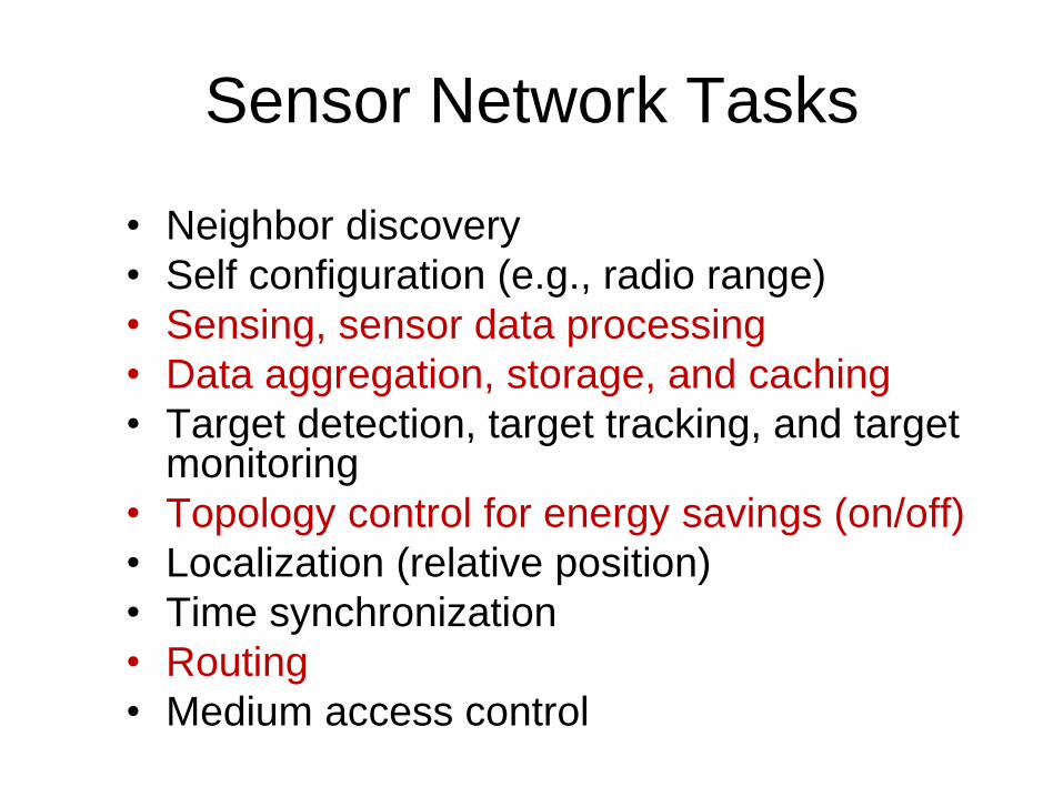
Sensor Network Tasks
• Neighbor discovery
• Self configuration (e.g., radio range)
• Sensing, sensor data processing
• Data aggregation, storage, and caching
• Target detection, target tracking, and target monitoring
• Topology control for energy savings (on/off)
• Localization (relative position)
• Time synchronization
• Routing
• Medium access control
Wireless Channel Conditions
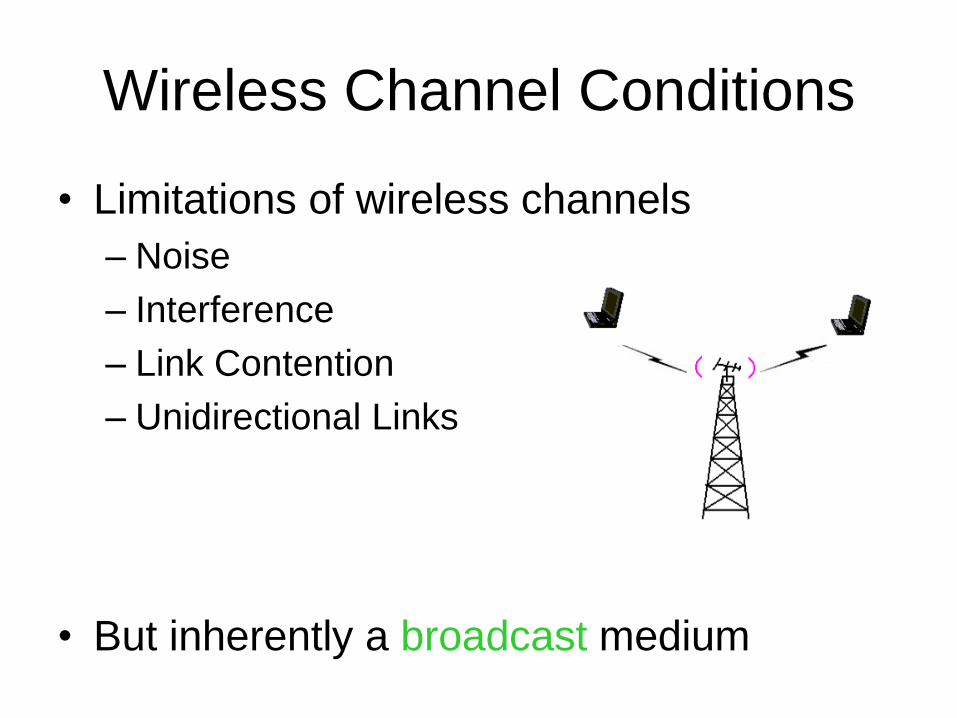
• Limitations of wireless channels
– Noise
– Interference
– Link Contention
– Unidirectional Links
• But inherently a broadcast medium
Constrained Resources
• No centralized authority
• Limited power – prolong life is a primary concern
• Wireless communication: more energy consumed and less reliable
• Limited computation and storage – lack of computation power/space affects the way security protocol is designed and caching/buffering can be performed.
• Limited input and output options – light/speaker only makes diagnosis difficult
Security Issues • Storing large keys is not practical but smaller
keys reduce the security
• More complicated algorithms increase security
but drain energy
• Sharing security keys between neighbors with
changing membership (due to node failure or
addition) needs a scalable key distribution and
key management scheme that is resilient to
adversary attacks
• Challenge is to provide security that meets the
application security requirements while
conserving energy
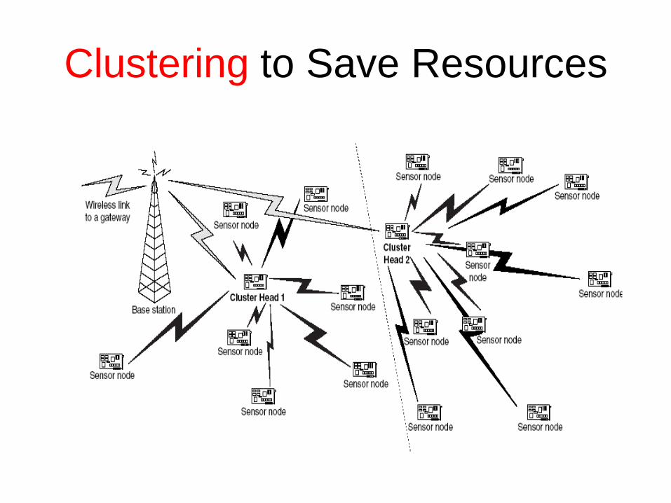
Clustering to Save Resources

Clustering
• Divide the network into a number of equal clusters each ideally containing the same # of nodes
• Cluster heads form a routing backbone
• Data aggregation: Combining cluster data readings into a single packet can save energy

Multihop Routing vs. Energy
• Multihop routing – reduces energy consumption (because energy consumed is roughly
proportional to square of distance)
– Introduces extra delay
• Energy consumed in transmitting a packet: – powering up the transmitter circuitry
– proportional to packet size
– proportional to square of distance
• How long should per-hop distance be? – if per-hop distance is too short, then
• Cost of powering up the transmitter circuitry dominates
– if per-hop distance is too long, then
• Cost of packet transmission dominates
• spatial reuse of bandwidth reduces
• overhead increases for state information maintenance and scheduling because the number of neighbors within a hop increases

LEACH Clustering • LEACH rotates cluster heads to balance energy
consumption
• Each cluster head performs its duty for a period of time
• Each sensor makes an independent decision in runs on whether to become a cluster head and if yes broadcasts advertisement packets
• Every node generates a random number (R) in [0,1] and computes a threshold T = P/(1-P*(r mod(1/P))). It decides to become a cluster head if R < T
– P: cluster head rotation probability (e.g. 5%)
– r: the current round # in the range of [0, 1/P - 1] since last time it is a cluster head

LEACH Clustering (cont.)
• Each sensor that is not a cluster head listens to
advertisements and selects the closest cluster head
• Once a cluster head knows the membership, a
schedule is created for the transmission from
sensors in the cluster to the cluster head to avoid
collision (e.g., based on TDMA)
• The cluster head can send a single packet to the
base station (directly) over long distance to save
energy consumption
• No assurance of optimal cluster distributions
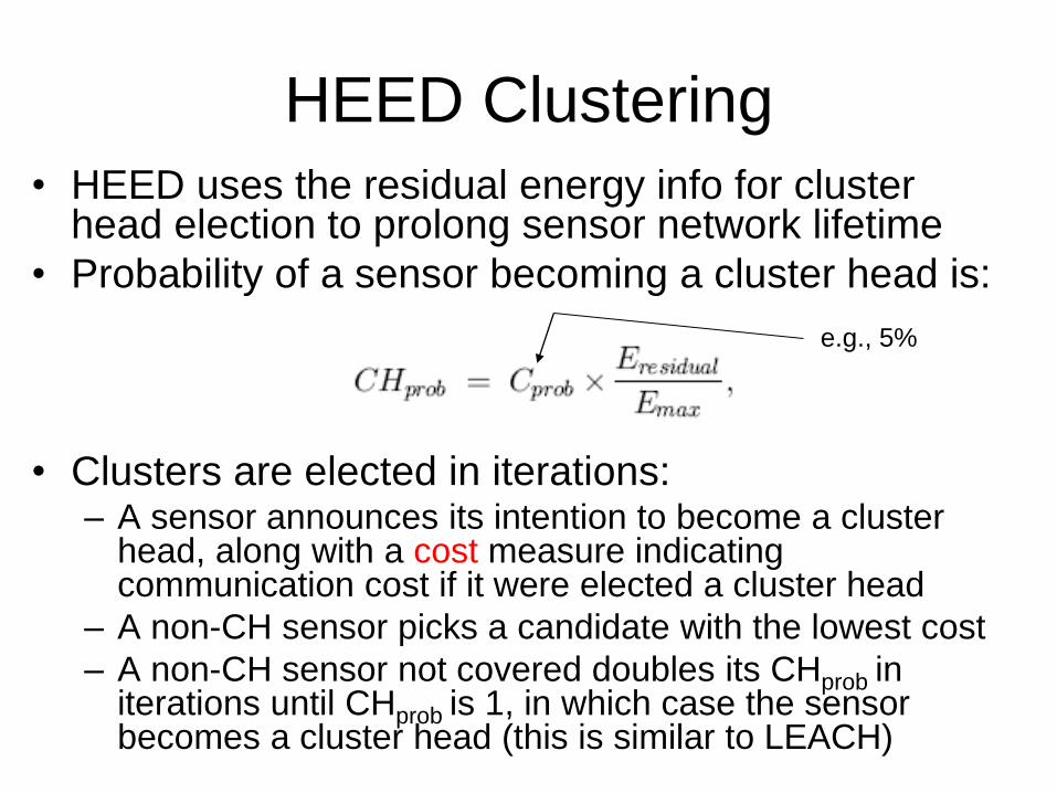
HEED Clustering
• HEED uses the residual energy info for cluster head election to prolong sensor network lifetime
• Probability of a sensor becoming a cluster head is:
• Clusters are elected in iterations: – A sensor announces its intention to become a cluster
head, along with a cost measure indicating communication cost if it were elected a cluster head
– A non-CH sensor picks a candidate with the lowest cost
– A non-CH sensor not covered doubles its CHprob in iterations until CHprob is 1, in which case the sensor becomes a cluster head (this is similar to LEACH)
e.g., 5%

PEGASIS
• A chain of sensors is formed for data transmission (could be formulated by the base station)
• Finding the optimal chain is NP-complete
• Sensor readings are aggregated hop by hop until a single packet is delivered to the base station: effective when aggregation is possible
• Advantages: No overhead of maintaining cluster heads and no long-distance data transmission
• Disadvantages: – Inefficiency in data aggregation: Can use tree instead
– Disproportionate energy depletion (for sensors near the base station): Can rotate parent nodes in the tree

Aggregation/Duplicate Suppression
• Aggregation of information in a tree
structure
– In-network information processing such as
max, min, avg
• Duplication Suppression:
– On forwarding messages, sensor nodes
whose values match those of other sensor
nodes can simply annotate the message
– Or just remain silent, on overhearing identical
(or ―similar enough‖) values

Querying a Sensor Network
• Can have sensor nodes periodically transmit
sensor readings
• More likely: Ask the sensor network a
question and receive an answer
• Issues:
– Getting the request out to the nodes
– Getting responses back from sensor nodes who
have answers
• Routing:
– Directed Diffusion Routing
– Geographic Forwarding (such as Geocasting)

Query-Oriented Routing
• For query-oriented routing: Queries are
disseminated from the base station to
the sensor nodes in a feature zone
• Sensor readings are sent by sensors to
the base station in a reverse flooding
order
• Sensor nodes that receive multiple
copies of the same message suppress
forwarding

Query: Asking a Question

Response to Base Station:
Initially

Directed Diffusion Routing
• Direction: From source (sensors) to sink (base station)
• Positive/negative feedback is used to encourage/discourage sensor nodes for/from forwarding messages toward the base station – Feedback can be based on delay in receiving data
– Positive feedback is sent to the first and negative feedback is sent to others
• A node will forward with low frequency unless it receives positive feedback
• This feedback propagates throughout the sensor network to suppress multiple transmissions
• Eventually message forwarding converges to the use of a single path with data aggregation for energy saving from the source to the base station

Responses, After Some Guidance
Use directed diffusion based on positive/negative feedback to
guide response message forwarding

Geographic Routing [Ref. 12]
• For dense sensor networks such that a sensor is available in the direction of routing
• Location of destination is sufficient to determine the routing orientation
• Research issue: – Selecting reliable paths for delivering messages
between sensors, or from sensors to a base station without excessively consuming energy
– Determining paths that avoid ―holes‖ – determining the boundary or perimeter of a hole through local information exchanges periodically to trade energy consumption (for hole detection) vs. routing efficiency

Geographic Forwarding

References
Chapters 8-11, F. Adelstein, S.K.S. Gupta, G.G. Richard III and L. Schwiebert, Fundamentals of Mobile and Pervasive Computing, McGraw Hill, 2005.
Other References:
11. X. Yu, “Distributed cache updating for the dynamic source routing protocol,” IEEE Transactions on Mobile Computing, Vol. 5, No. 6, pp. 2006, pp. 609-626.
12. S. Wu and K.S. Candan, “Power-Aware Single and Multipath Geographic Routing in Sensor Networks,” Ad Hoc Networks, Vol. 5, 2007, pp. 974–997.