lecture 5 comp of treatments and anovaee290h/fa05/lectures/pdf/lecture 5 co… · lecture 5:...

Lecture 5: Comparison of Treatments and ANOVA

SpanosEE290H F05

1


SpanosEE290H F05

2

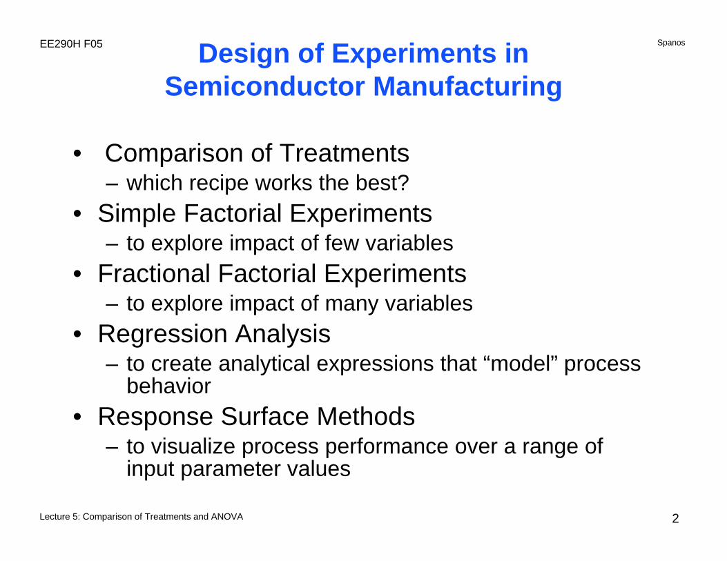
Design of Experiments inSemiconductor Manufacturing

• Comparison of Treatments– which recipe works the best?

• Simple Factorial Experiments – to explore impact of few variables

• Fractional Factorial Experiments – to explore impact of many variables

• Regression Analysis– to create analytical expressions that “model” process

behavior• Response Surface Methods

– to visualize process performance over a range of input parameter values


SpanosEE290H F05

3

Design of Experiments

• Objectives:– Compare Processing Recipes– Find the Parameters that Matter– Create Models to Predict Process Results

• Problems:– Experimental / Measurement Error– Confusion of Correlation with Causation– Complexity of the Effects we study


SpanosEE290H F05

4

Problems Solved

• Compare Recipes– Choose the recipe that gives the best results– Organize experiments to facilitate the analysis– Use experimental results to build process models– Use models to optimize the process


SpanosEE290H F05

5

Comparison of Treatments

• Internal and External References• The Importance of Independence• Blocking and Randomization• Analysis of Variance


SpanosEE290H F05

6

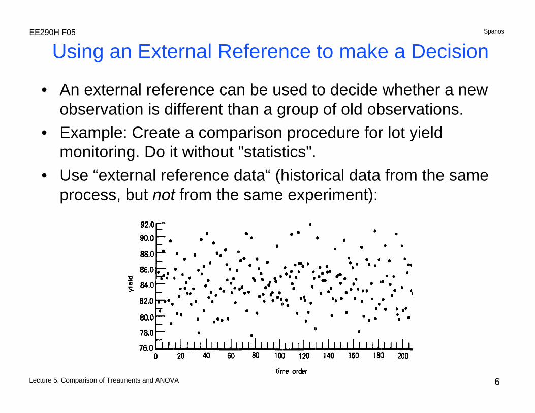
Using an External Reference to make a Decision

• An external reference can be used to decide whether a new observation is different than a group of old observations.

• Example: Create a comparison procedure for lot yield monitoring. Do it without "statistics".

• Use “external reference data“ (historical data from the same process, but not from the same experiment):


SpanosEE290H F05

7

To compare the difference between the average of successive groups of ten lots, I build the histogram from the reference data:

Example: Using an External Reference

• Each new point can then be judged on the basis of the reference data.

• The only assumption here is that the reference data is relevant to my test!

Points generated by the “good” process

that fail the test(type I error)


SpanosEE290H F05

8

Using an Internal Reference...

• We could generate an "internal" reference distribution from the very data we are comparing.

• Sampling must be random, so that the data is independently distributed.

• Independence would allow us to use statistics such as the arithmetic average or the sum of squares.

• Internal references are based on Randomization.


SpanosEE290H F05

9

121086420630

640

650

660

Etch

Rat

e

660650640630620Etch Rate

Rec

ipe

Type

A

B

Randomization Example

• Is recipe A different than recipe B?

Sample

A B

XBXA


SpanosEE290H F05

10

Randomization Example - cont.

• There are many ways to decide this...1. External reference distribution (based on old data.)2. Assumed, approximate external reference distr. (such as

student-t, normal, etc).3. Internal reference distribution.4. "Distribution free" tests.

• Options 2, 3 and 4 depend on the assumption that the samples are independently distributed.


SpanosEE290H F05

11

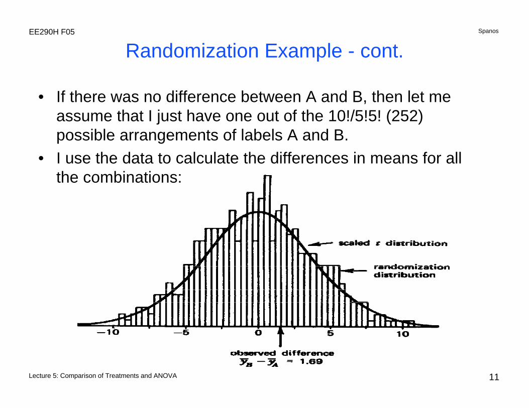
Randomization Example - cont.

• If there was no difference between A and B, then let me assume that I just have one out of the 10!/5!5! (252) possible arrangements of labels A and B.

• I use the data to calculate the differences in means for all the combinations:


SpanosEE290H F05

12

t0 = (yB -yA) - (μA - μB)

s 1nA

+ 1nB

The student-t distribution was, in fact, defined to approximate such randomized distributions, when the “parent” distribution is normal!

The Origin of the student-t Distribution

• For the etch example, t0 = 0.44 and Pr (t > t0) = 0.34• Randomized Distribution = 0.33


SpanosEE290H F05

13

A B A

B A

B B

B

B A

A B

B A

A B

B A

Random Blocked

A A

Example in Blocking

• Compare recipes A and B on five machines. • If there are inherent differences from one machine to the

other, what scheme would you use?


SpanosEE290H F05

14

d - δsd/ n

~ tn-1

d = ±d1±d2±d3±d4±d5

5

In general, randomize what you don't knowand block what you do know.In general, randomize what you don't knowand block what you do know.

Example in Blocking - cont.

• With the blocked scheme, we could calculate the A-B difference for each machine.

• The machine-to-machine average of these differences could be randomized.


SpanosEE290H F05

15

660650640630620610Etch Rate

Rec

ipe

Type

A

B

C

D

Your Question: Are the four treatments the same or not?Your Question: Are the four treatments the same or not?

Analysis of Variance

The Statistician's Question: Are the discrepancies betweenthe groups greater than the variation within each group?

The Statistician's Question: Are the discrepancies betweenthe groups greater than the variation within each group?

XA

XA

XA

XA


SpanosEE290H F05

16

i=1 i=2 i=3 i=4 i=5 Avg st2 νt

1: 650 648 632 645 641 643.20 202.80 4 25.002: 645 650 638 643 640 643.20 86.80 4 25.003: 623 628 630 620 618 623.80 104.80 4 207.364: 645 640 648 642 638 642.60 63.20 4 19.36

sR2 =

sT2 =

sT2

sR2 =

(yt - y)2

Calculations for our Example


SpanosEE290H F05

17

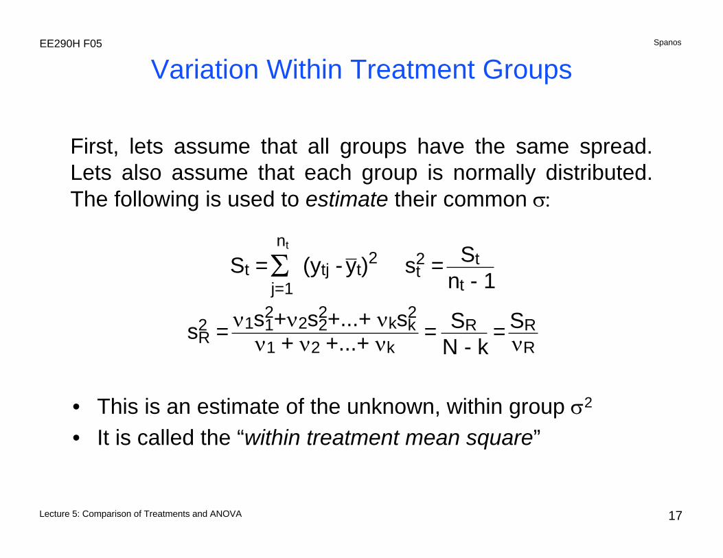
St = (ytj - yt)2Σj=1

nt

st2 = St

nt - 1

sR2 = ν1s1

2+ν2s22+...+ νksk

2

ν1 + ν2 +...+ νk= SR

N - k= SR

νR

First, lets assume that all groups have the same spread. Lets also assume that each group is normally distributed. The following is used to estimate their common σ:

Variation Within Treatment Groups

• This is an estimate of the unknown, within group σ2

• It is called the “within treatment mean square”


SpanosEE290H F05

18

sT2 =

nt(yt - y)2Σt=1

k

k - 1= ST

νT

If all the treatments are the same, then the within and between treatment mean squares are estimating the same number!

If all the treatments are the same, then the within and between treatment mean squares are estimating the same number!

This is the between treatment mean square

Variation Between Treatment Groups

• Let us now form Ho by assuming that all the groups have the same mean.

• Assuming that there are no real differences between groups, a second estimate of sT

2 would be:


SpanosEE290H F05

19

sT2 estimates σ2 + nt τt

2Σt = 1

k/ (k - 1)

where τt ≡ μt - μ

If the treatments are different then:

What if the Treatments are different?

In other words, the between treatment mean square is inflatedby a factor proportional to the spread among the treatments!In other words, the between treatment mean square is inflatedby a factor proportional to the spread among the treatments!


SpanosEE290H F05

20

sT2

sR2 is significantly greater than 1.0

This can be formalized since:sT

2

sR2 ~ Fk-1, N-k

Therefore, the hypothesis of equivalence is rejected if:

Final Test for Treatment Significance


SpanosEE290H F05

21

SD = (ytj - y)2Σj=1

nt

Σt=1

ksD

2 = SDN - 1

= SDνD

Obviously (actually, this is not so obvious, but it can be proven):

SD = ST + SR and νD = νT + νR

A measure of the overall variation:

More Sums of Squares


SpanosEE290H F05

22

Source Sum of DFs Mean square of Var squares

between ST vT (k-1) sT

within SR vR (N-k) sR

total SD vD (N-1) sD

2

2

2

ANOVA Table


SpanosEE290H F05

23

Source Sum DFs Mean sq of Var of sq

average SA vA ( 1 ) sA

between ST vT (k-1) sT

within SR vR (N-k) sR

2

2

2

total S v ( N )

ANOVA Table (full)


SpanosEE290H F05

24

Data File:

SourceSum of

SquaresDeg. of

FreedomMean

Squares F-Ratio Prob>F

CompEtch

BetweenRecipe

Error

Total

1.38e+3

4.58e+2

3

16

4.61e+2

2.86e+1

1.61e+1

1.84e+3 19

4.29e-5

Anova for our example...


SpanosEE290H F05

25

Y = A + T + R

In Vector Form:

yti y yt - y yti - yt

.

.

.

.

.

.

.

.

.

.

.

.

= + +

N 1 k-1 N-k

Decomposition of Observations

The term degrees of freedom refers to the dimensionality of the space each vector is free to move into.


SpanosEE290H F05

26

Y = A + DEasy to prove that A ⊥ D.

D = R +TEasy to prove that R ⊥ T and A ⊥ R.

Y

A T

YD R

Geometric Interpretation of ANOVA


SpanosEE290H F05

27

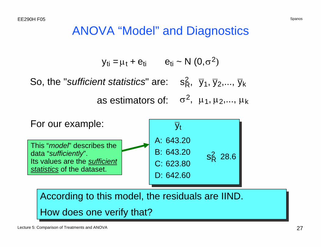
So, the "sufficient statistics" are: sR2 , y1, y2,..., yk

yti = μt + eti eti ~ N (0, σ2)

σ2, μ1, μ2,..., μkas estimators of:

sR2

ytFor our example:

According to this model, the residuals are IIND. How does one verify that?

According to this model, the residuals are IIND. How does one verify that?

ANOVA “Model” and Diagnostics

A: 643.20B: 643.20C: 623.80D: 642.60

28.6This “model” describes the data “sufficiently”.Its values are the sufficientstatistics of the dataset.


SpanosEE290H F05

28

Are these recipes significantly different?

Analysis of VarianceSourceModelErrorC Total

DF5

227232

Sum of Squares269705841985388

Mean Square5394257

F Ratio20.96Prob > F

0.0000

5060708090

100110120130140150160170180190200

E B C D A FRecipe

ANOVA Example: Poly Deposition

Thic

knes

s in

nm


SpanosEE290H F05

29

Residual thick.

-40 -30 -20 -10 0 10 20 30 40

Residual thick.

-40 -30 -20 -10 0 10 20 30 40

Residual thick.

-40 -20 -10 0 10 20 30 40

Residual thick.

-40 -30 -20 -10 0 10 20 30 40

Residual Plots:


SpanosEE290H F05

30

Residualthick.

-40-30-20-10

0102030405060708090

E B C D E F

Deposition RecipeV1 V2

Wafer Vendor

Residual Plots (cont):


SpanosEE290H F05

31

ANOVA Summary

• Plot Originals• Construct ANOVA table• Are the treatment effects significant?• Plot residuals versus:

– treatment– group mean– time sequence– other?

• ANOVA is the basic tool behind most empirical modeling techniques.

lecture 5 comp of treatments and anovaee290h/fa05/lectures/pdf/lecture 5 co… · lecture 5:...

Documents