LECTURE 5: Discrete random variables:

probability mass functions and expectations

• Random variables: the idea and the definition

- Discrete: take values in finite or countable set

• Probability mass function (PMF)

• Random variable examples

Bernoulli

Uniform

Binomial

Geometric

• Expectation (mean) and its properties

The expected value rule

Linearity 1

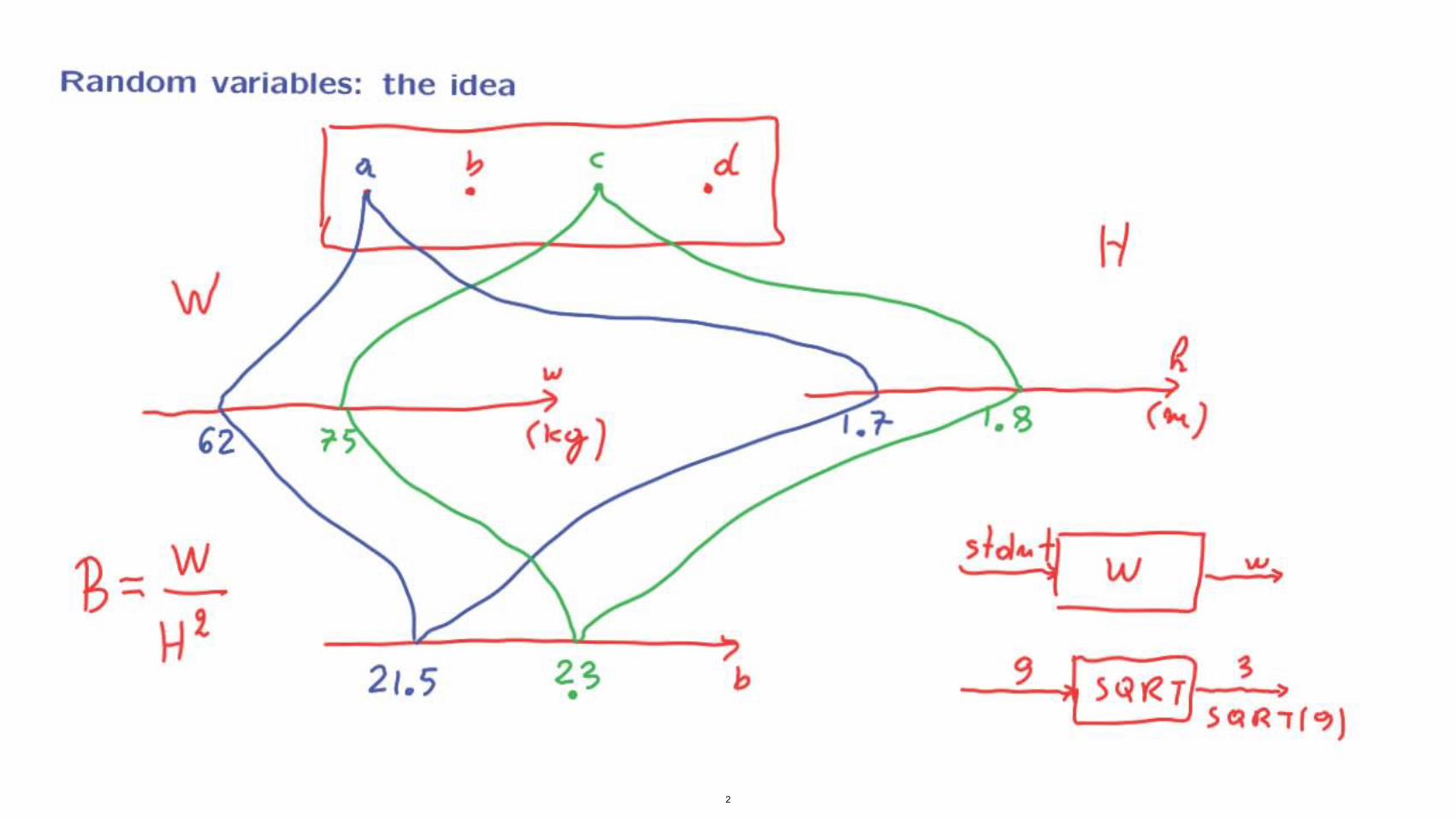
Random variables: the idea

23•

c d.•

1--1

sid.. L,--, W -, "'.

b 9

2

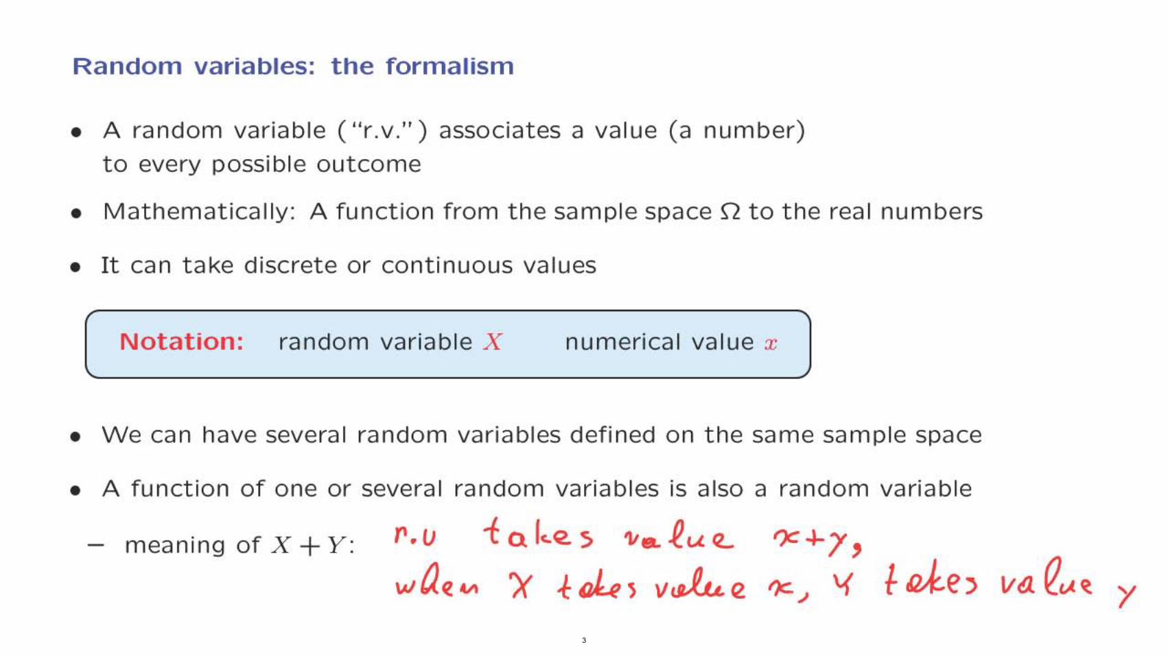
Random variables: the formalism

• A random variable ("r.v,") associates a value (a number)

to every possible outcome

• Mathematically: A function from the sample space Sl to the real numbers

• It can take discrete or continuous values

Notation: random variable X numerical value x

• We can have several random variables defined on the same sample space

• A function of one or several random variables is also a random variable

-t 0. k<2. 5 'II.. ~ c..£ "­- meaning of X + Y:

')( ik) v.J.ue. 3

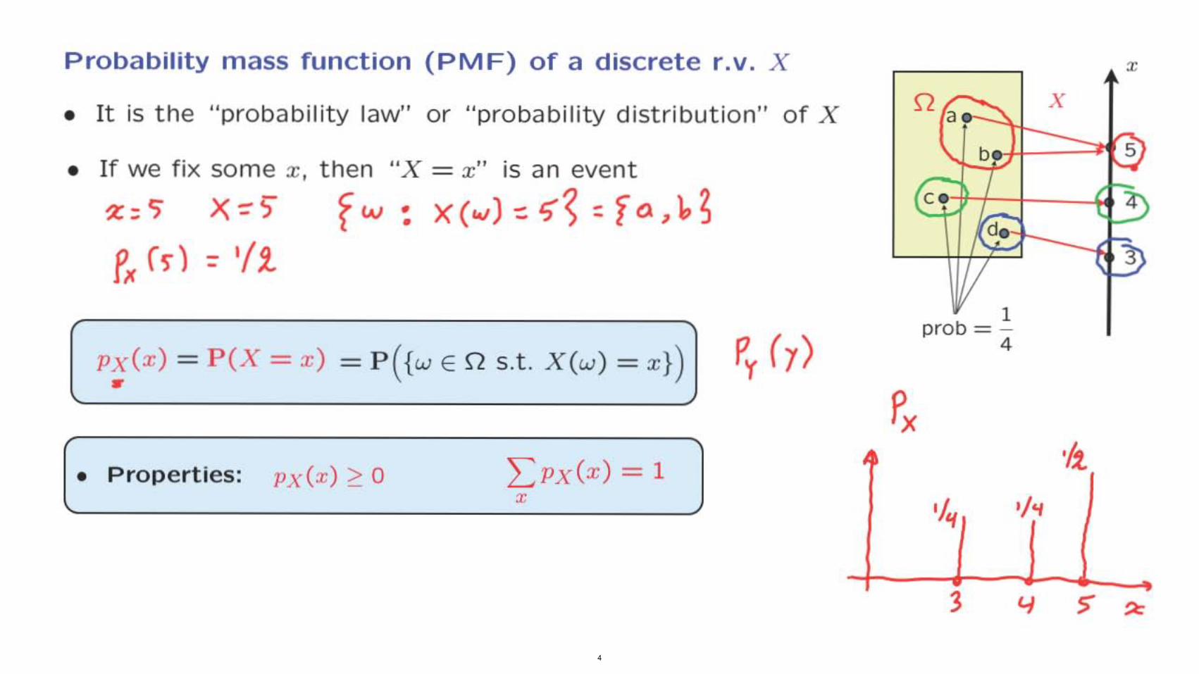
Probability mass function (PMF) of a discrete r.v. X x

x• It is the " probability law" or "probability distribution" of X

• If we fix some x, then "X = x" is an event

><;=5" fw : XC...)" ~~ =fa,),s fiC (5") = '(i

prob =­

PX(x ) = P(X = x ) = p( {w E >2 S.t. X(w) = x}) P'f (7) 4

" Px

>2 a •

1

• Properties: px(x) > 0 L>X(x) = 1 x

'/1. ./'1 ./~

4

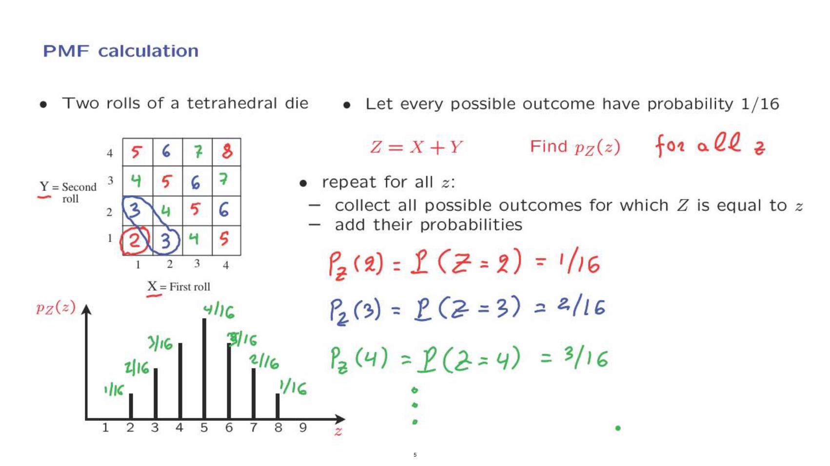
PMF calculation

• Two rolls of a tetrahedral die • Let every possible outcome have probability 1/ 16

4 ;- , 1 3 'i , , 2

, '1

3

x == First roll -

!> .. b , 4

z=x+y Find pz(z) fo~ 0. ell.. ~ • repeat for all z:Y == Secund

- roll - collect all possible outcomes for which Z is equal to z - add their probabilities

Pl- (~) =1. (2- :. 2) :- '/1 G

pz(z) Pz. (:l» : f.. (2- = '5) -" 2.11 b

'I.(t" Pa (4) -;1(2:::.4) = 3/16

•• • • 5

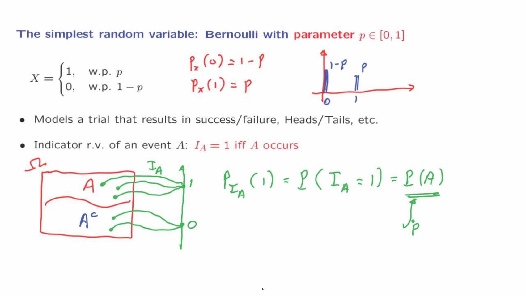
The simplest random variable: Bernoulli with parameter p E [0 , 1)

f. (<» :> 1 - f 1-1' px = 1 , w .p . p 0 , w .p . 1 - p '1',,(1):: p H

I

• Models a tria l t hat resu lts in success/ fai lu re, Heads/ T ai ls, et c.

• Indicat or r .v . o f an event A: I A = 1 iff A occu rs

o

6

• • • • • •

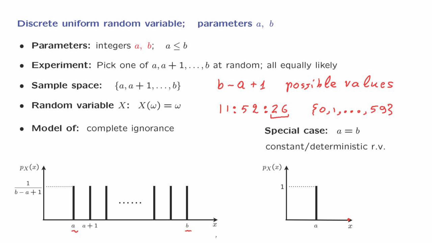
Discrete uniform random variable; parameters a, b

• Parameters: integers a, b; a < b

• Experiment: Pi ck one of a , a + 1, ... , b at random ; all equa ll y likely

• Sample space: {a , a + 1, ... , b} b -Q + ~

• Random variable X : X(w) = w

• Model of: com p let e ignorance Special case: a = b

const ant/ det erministi c r .v.

xPx ( )

1

px(x)

1 ............ . b a+ 1

. . . . . . . . . . . . ,

xb a x-7

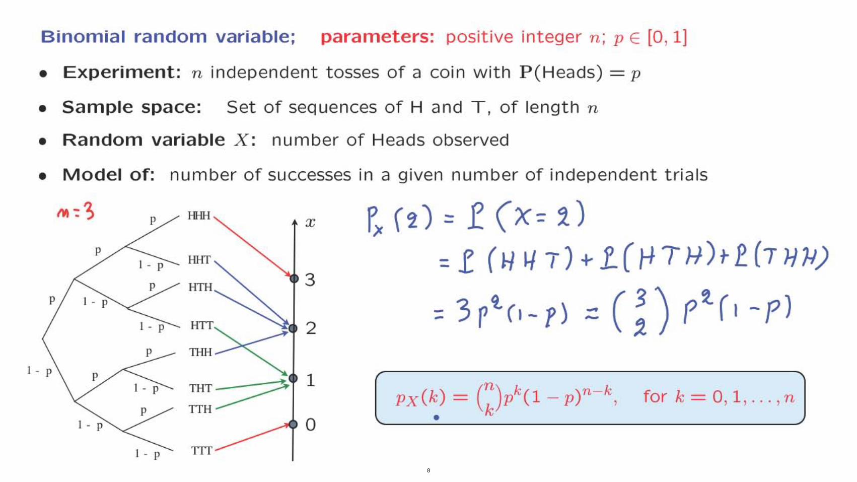
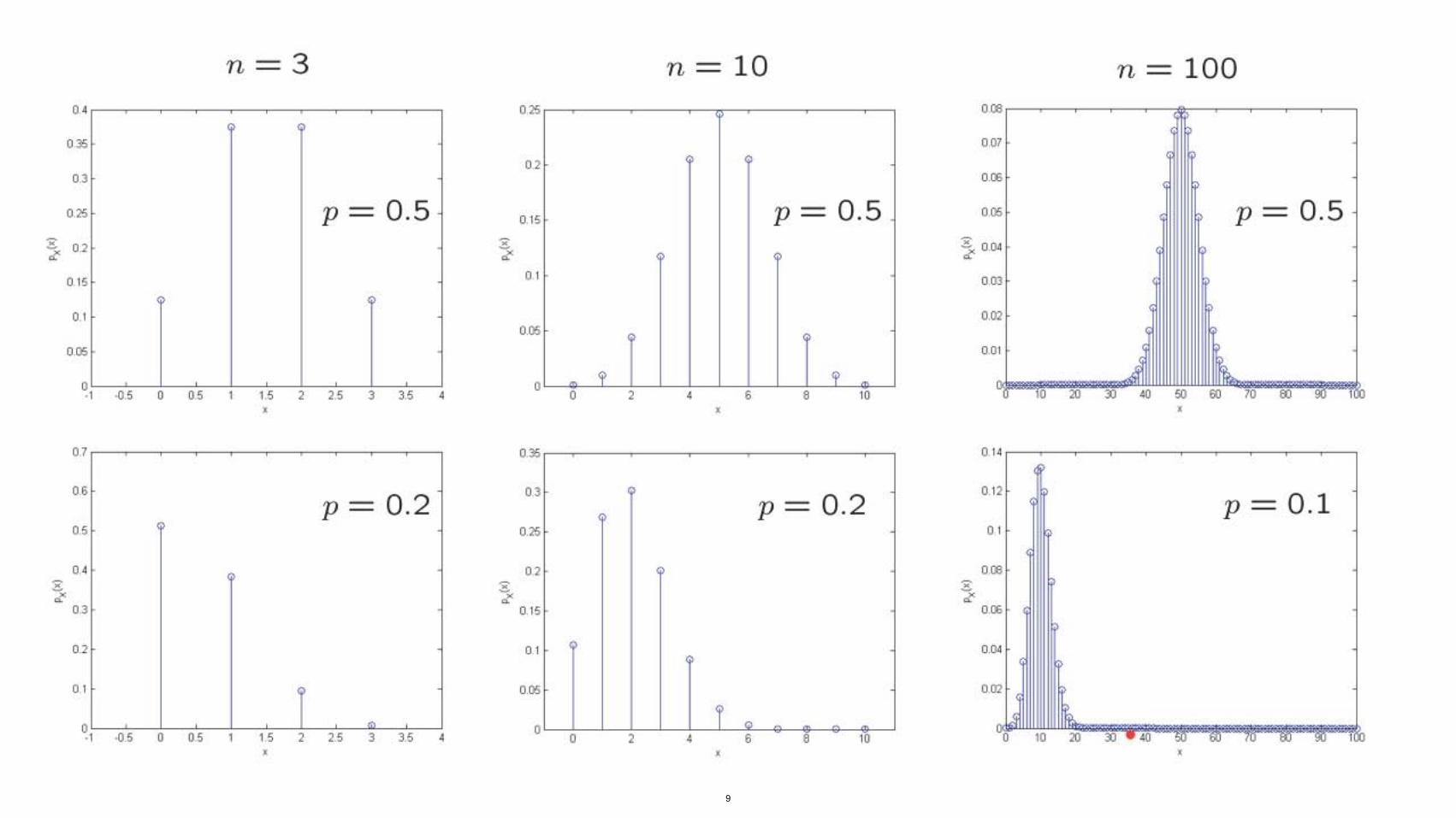
Binomial random variable; parameters: positive integer n; p E [0 , 1]

• Experiment: n independent tosses of a coin with P(Heads) = p

• Sample space: Set of sequences of Hand T, of length n

• Random variable X: number of Heads observed

• Model of: number of successes in a given number of independent trials

1-11-11-1p x Px(2)=f(X=2) HI-IT =.f (HI·/T)+l(HTH)I-£(TlI]1)1 - P

P 1m,

____

3 P 1 - P

1 - P H1T 2 P UlH

1 - P

1 1 - P HIT ­

ITHP o

TIT1 - P 8

••

••

n 3 n 10 n 100 •, .. ••

•,•, p - 0.5-•• p 0.5p - 0.5, -" ,

", •,

•, •••• ." •, ., • .. ,

" ,

" ,

" , • , ,

• , , • • " , , ,

.. ,• -p - 0.2 p - 0.2.. .. .. •, , •,"

" !·,c-c.", -;.-,.",, -j,-""-',c-,,,,-;,c-,,",,-j, ,

, .~• ,

, • • ,

p - 0. 1 " "

9

k

p

J):~oo

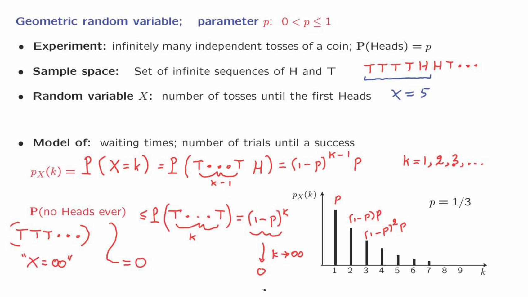
Geometric random variable; parameter p: 0 < p < 1

• Experiment: infinitely many independent tosses of a coin; P(Heads) = p

-rTTTI-IHT •••• Sample space: Set of infinite sequences of Hand T ( ,

• Random variable X: number of tosses until the first Heads

• Model of: waiting times; number of trials until a success

px(k) = 1 (X:: ~) =1 (~T J1 ') ::c "- p{-' p l< - ,

p = 1/ 3 P(no Heads ever) r·- p)f 1; ­

(._1"1 I'~TI'" ..)

"x ::.09·f 123456789 ko

10

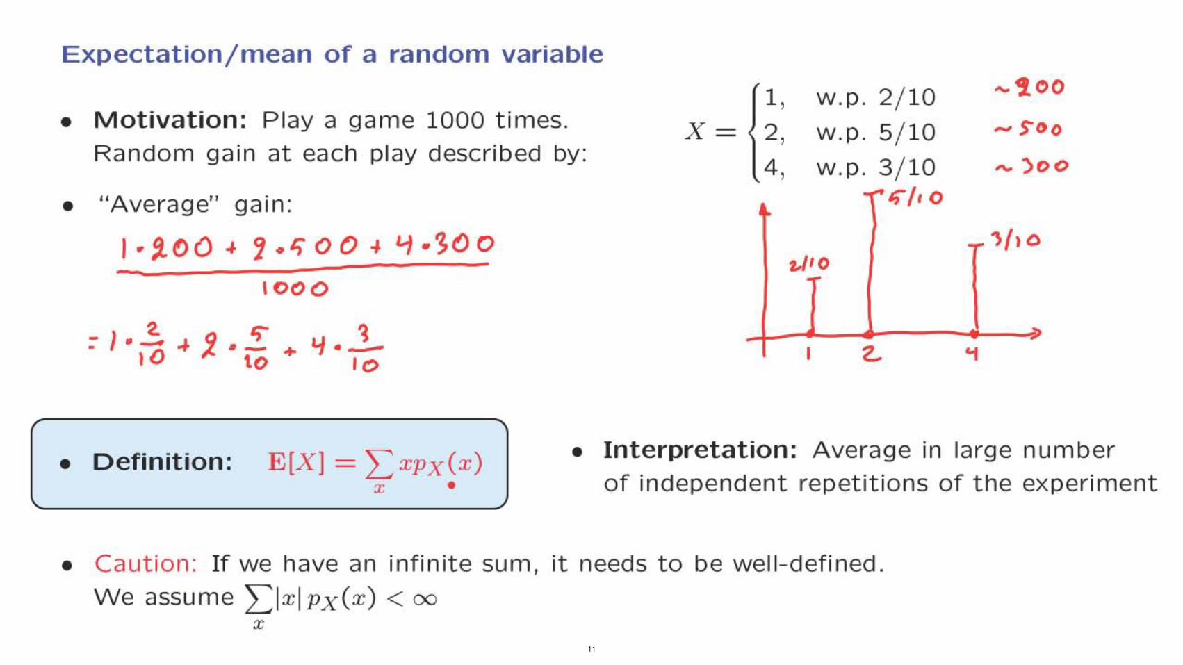
Expectation/mean of a random variable

• Motivation: Playa game 1000 times. Random gain at each play described by:

• "Average" gain:

I'~OO. 7.<;00 ~ '1.~oo .

1000

-I.~ .. Q , ~ y. ­- 0 ~.-+I to Ie:> I '1

• Interpretation: Average in large number• Definition:

of independent repetitions of the experimentx

• Caution: If we have an infinite sum, it needs to be well-defined.

We assume 2:lx lpx(x) < 00

x 11

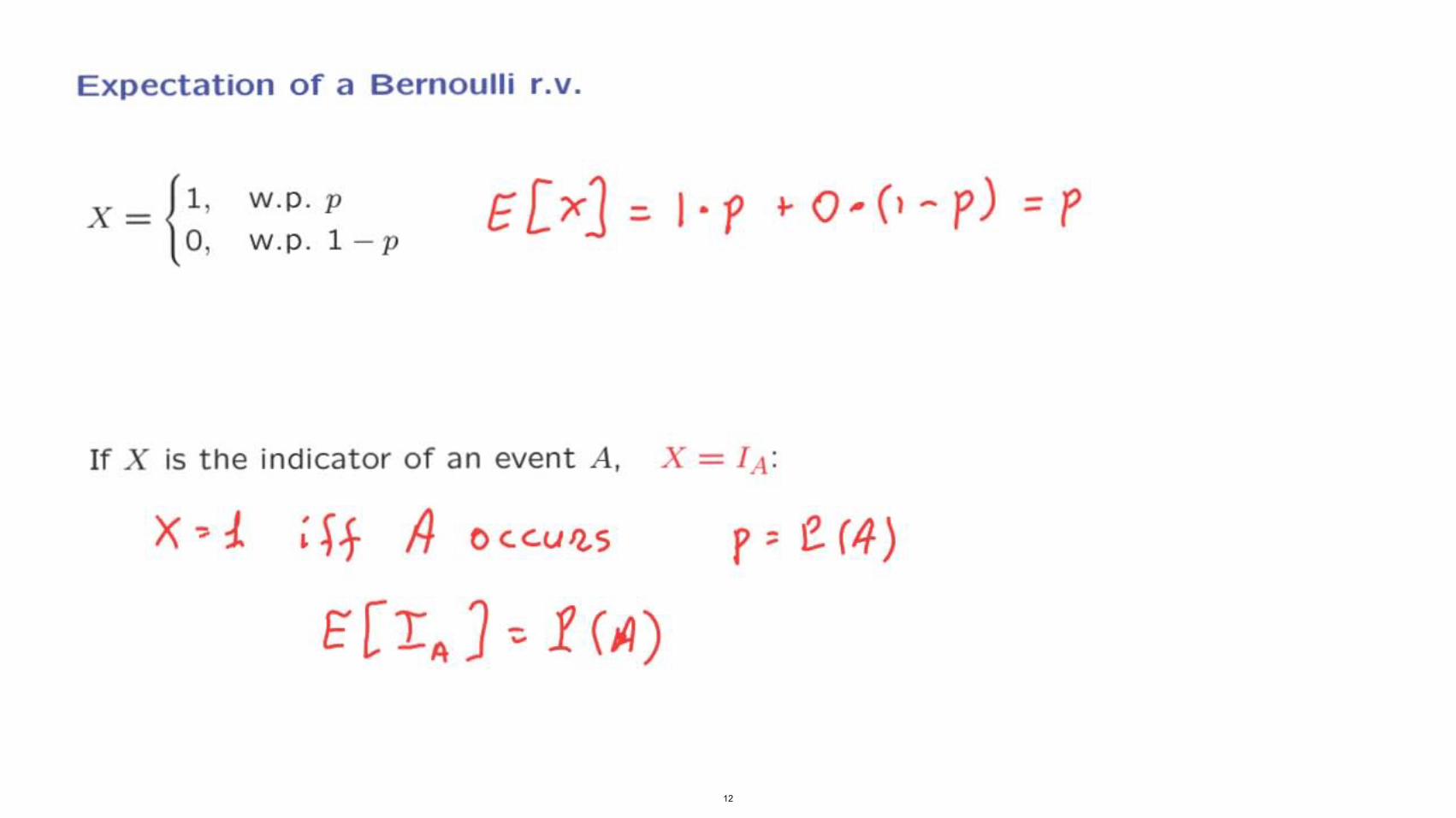
Expectation of a Bernoulli r.v.

1, w.p_ p X=

0 , w.p. 1 - p

If X is the indicator of an event A. X = IA:

x ~ :! ; if IJ 0 c. c.u1.5 r ' e. (4)

E[IA ] ~ .f (jI))

12

• • • • ••

Expectation of a uniform r.v .

• Uniform on O, l , ... , n

p (x )x

1

n +1

• Definition: E[X] = L XPX (x ) x

n x0 1

, , E[X] = 0--+1--' -

, ........ , ""+1

, :0 --_ (!)+ 1+ •• _ +"") :: _'_.• "" (""+d =

"" + , 2

13

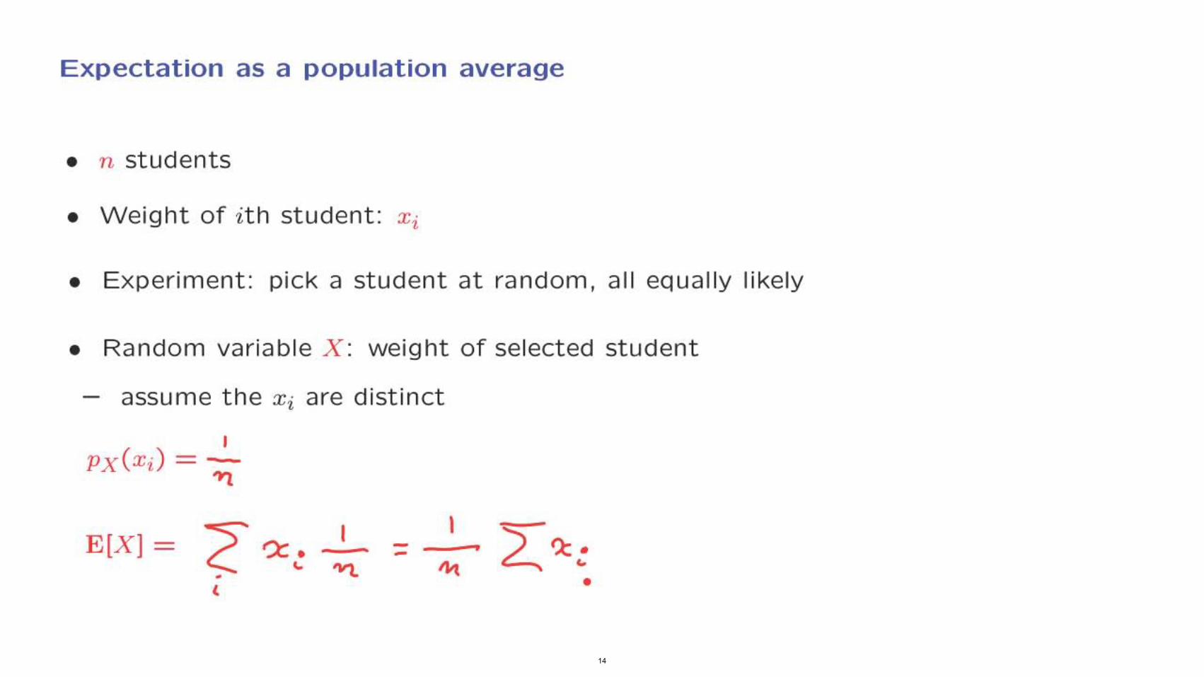
Expectation as a population average

• n students

• Weight of i th student: xi

• Experiment: pick a student at random, all equally likely

• Random variable X : weight of selected student

- assume the Xi are distinct

J PX(Xi) = - ­

'>1

IE[X] = ­-, "'l.

14

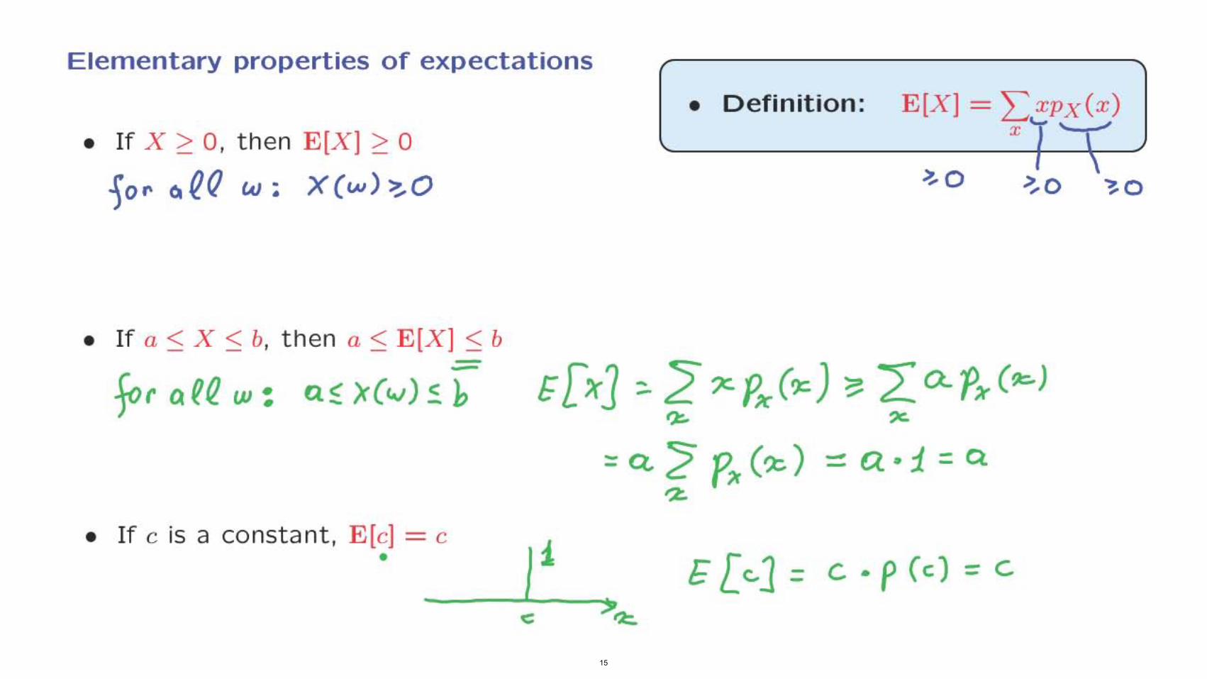
Elementary properties of expectations

• If X > 0 , th e n E[X) > 0

10r Co~!l w; X (w) >--0

• If a < X < b, th en a < E[X) < b -

• Definition: E[X) = LXPX(x) x

>"0

for 0, eQ. w: 0.0'(",) ~ h :: Q. ;? p" (>;t:.) ~ a. -1. =Q

'Z

• If c is a co nst a nt , E[c) = •

c

15

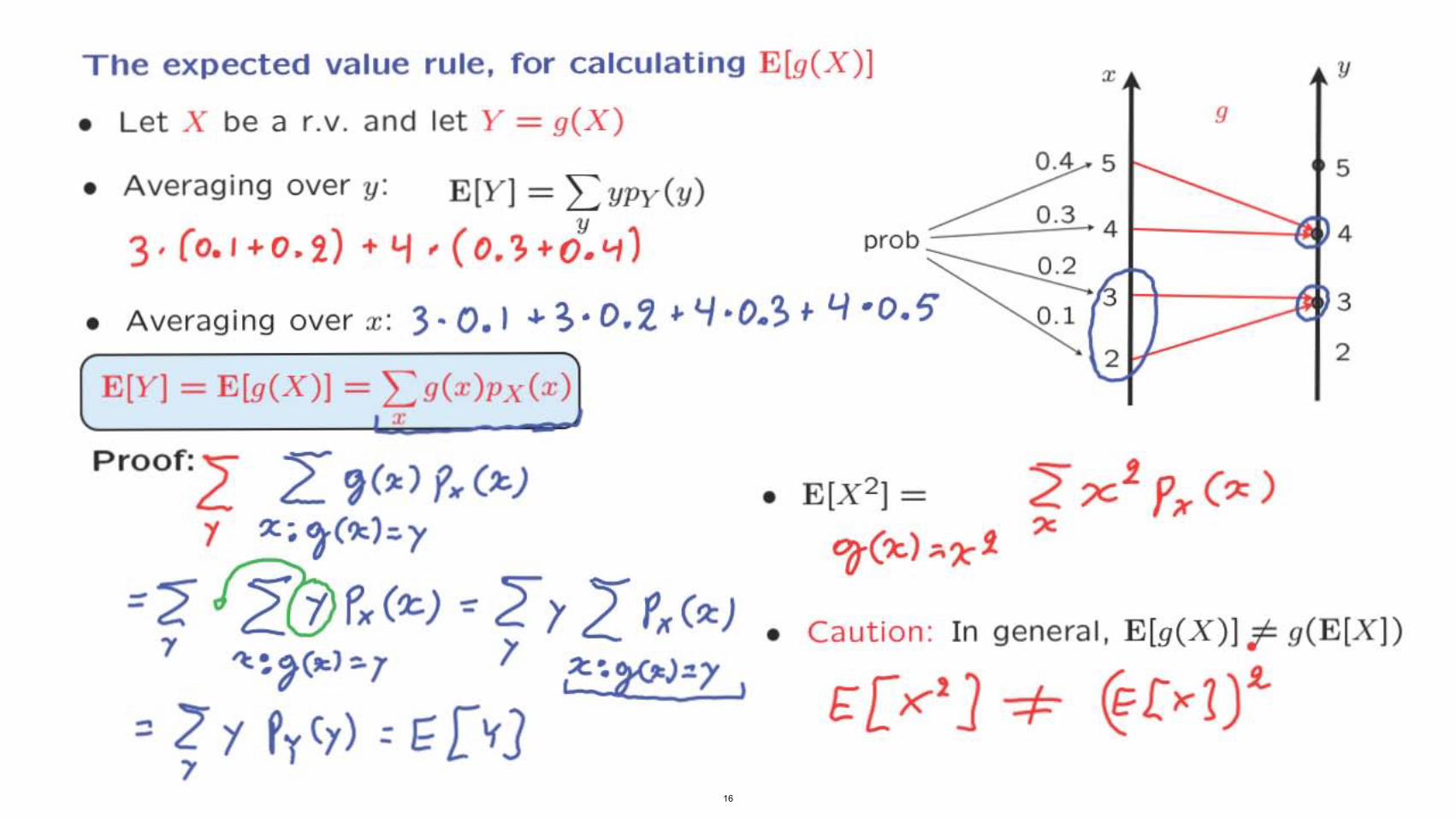
The expected value rule. for calculating E [g(X) ]

Lj '0.5 2

yx

9• Let X be a r.v. and let Y = g(X) 0.4 5 5

• Averaging over y: E[Y] = L YPY(Y) y 43,(0.1+0.2) +'1,(0.3+0.'11

3• Averaging over x: 3· o. I ... ~. 0.2' Y·0.> t

2 E [Y] = E[g(X)] = Lg(x)pX(x) ~__________ T~_____~

prOOf:.z L ~(!l:) f'.. C"-) • E[X2] = 'f It; '(~):.)' ~(?:) ,,~i

::~ ~ 1, f,,(2:) -:: :2., Z fx(~) • Ca ution: In general, E[g(X) ] ~ g(E[X])

"1 'I;~,("'l=1 7 ,;t:~~)"i' I

£ [)<"2] -=F @[><1).t.'" LY fyCr) =f[If]

")' 16

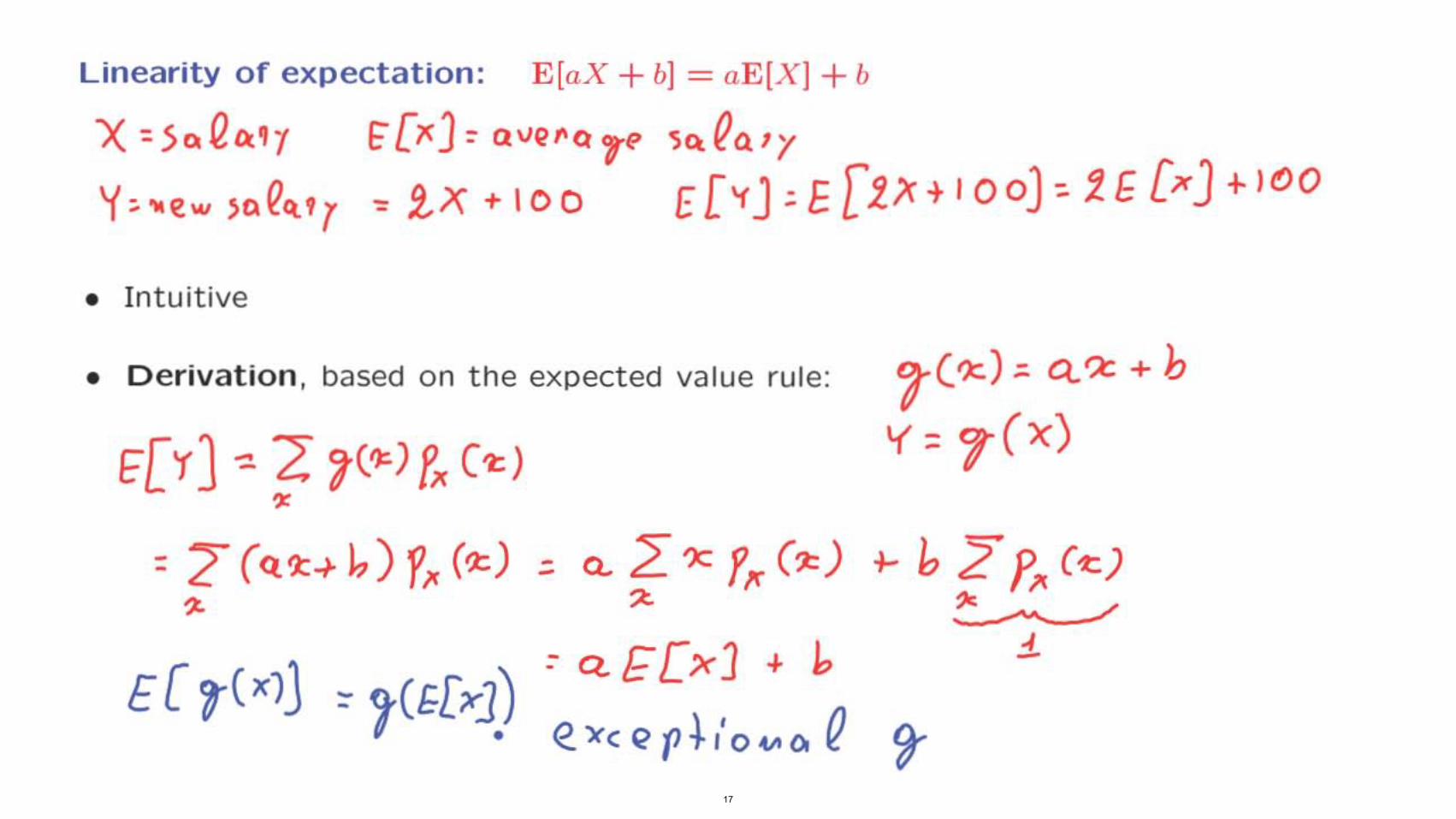
Linearity of expectation: E[aX + bl = aE[XI + b

")( =5o.Qa:?1 r:[}(] 0 Qve~Q"1? 5Ct.eo.'y

y , ..e'" )0 e~,r ~ i X + I 0 0 E[ '{J ; E[2. X+I 0 oJ : 2 f [;rJ + ) 0 0

• Int uit ive

• Derivation , based on the expected value rule: pC-:1:) ::. a. ':C + h

l( =,,(x)

=L (Q.9:~ 1,) y" (-:1:) ; a. 2>: 1'1< ('J;) +- h 2' PI< (t) ". ?< ?-.-... ./

:1..

• e."lee Q p+io",Oo ~ 17

MIT OpenCourseWarehttps://ocw.mit.edu

Resource: Introduction to ProbabilityJohn Tsitsiklis and Patrick Jaillet

The following may not correspond to a particular course on MIT OpenCourseWare, but has been provided by the author as an individual learning resource.

For information about citing these materials or our Terms of Use, visit: https://ocw.mit.edu/terms.