LECTURE 5: DUALITY AND SENSITIVITY ANALYSIS1. Dual linear program

2. Duality theory

3. Sensitivity analysis

4. Dual simplex method

Introduction to dual linear program

• Given a constraint matrix A, right hand side vector b, and

cost vector c, we have a corresponding linear

programming problem:

• Questions:

1. Can we use the same data set of (A, b, c) to construct

another linear programming problem?

2. If so, how is this new linear program related to the

original primal problem?

Guessing

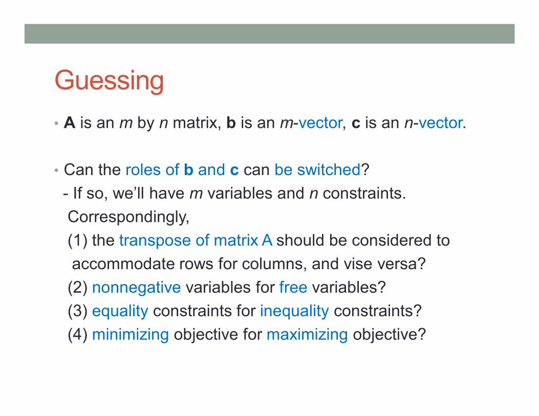
• A is an m by n matrix, b is an m-vector, c is an n-vector.

• Can the roles of b and c can be switched?

- If so, we’ll have m variables and n constraints.

Correspondingly,

(1) the transpose of matrix A should be considered to

accommodate rows for columns, and vise versa?

(2) nonnegative variables for free variables?

(3) equality constraints for inequality constraints?

(4) minimizing objective for maximizing objective?

Dual linear program

• Consider the following linear program

• Remember the original linear program

Example

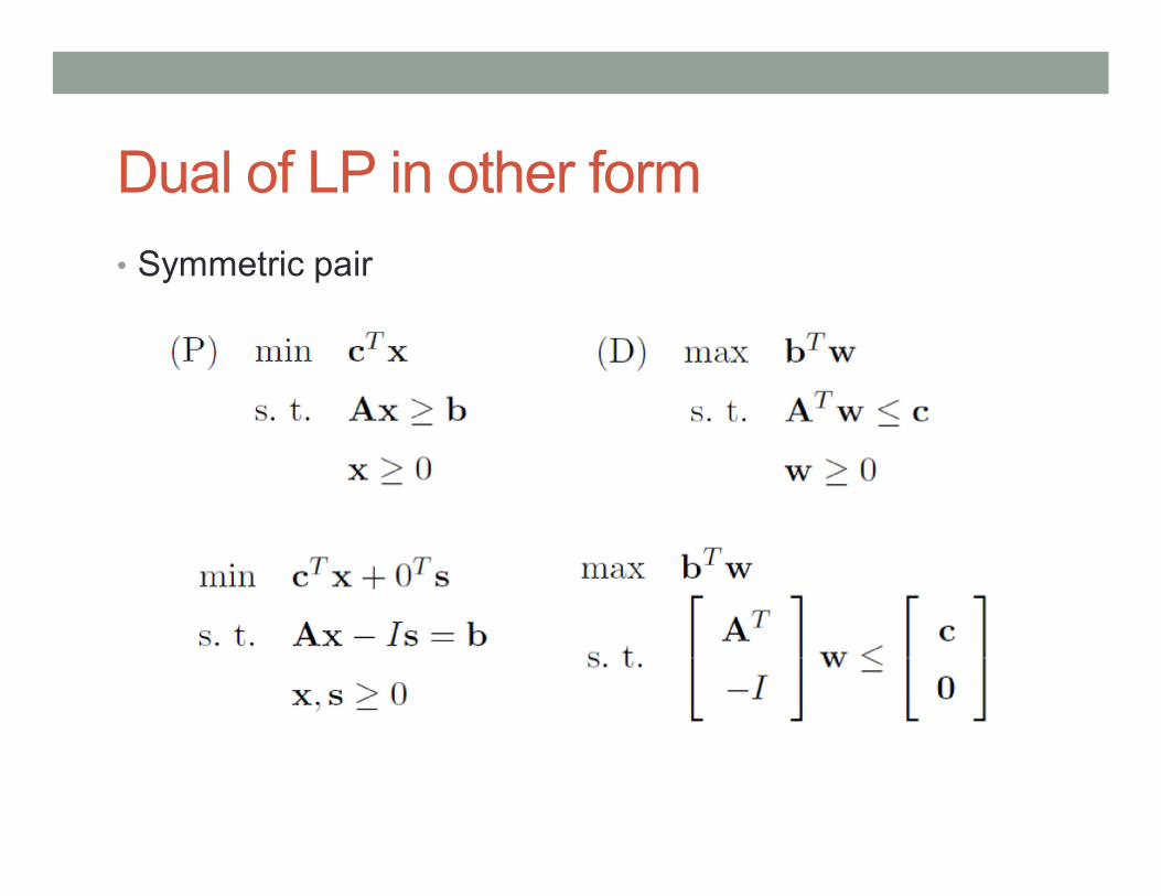
Dual of LP in other form

• Symmetric pair

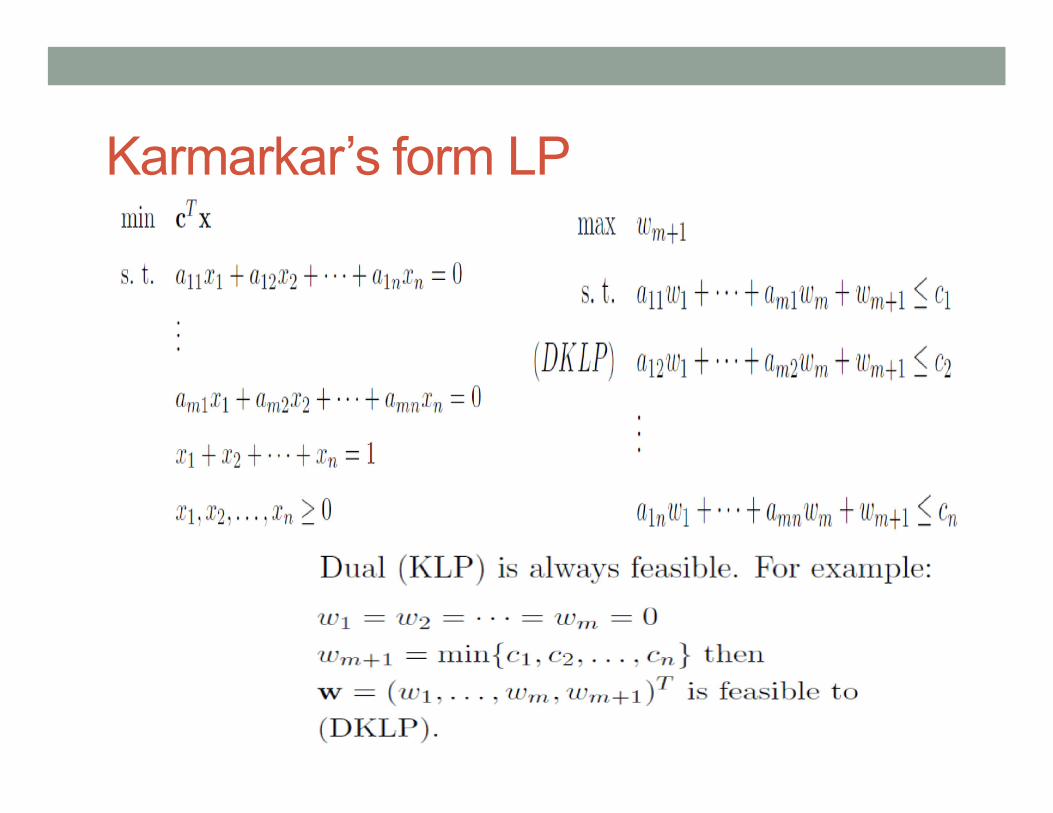
Karmarkar’s form LP

How are they related ?

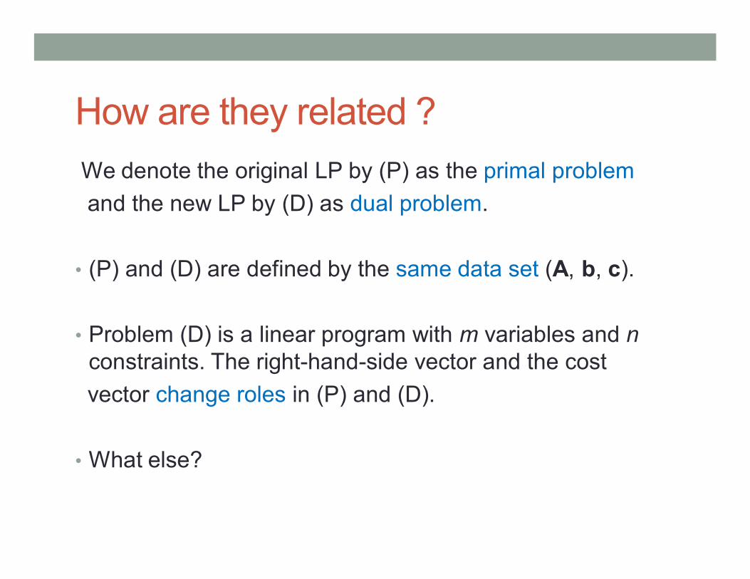
We denote the original LP by (P) as the primal problem

and the new LP by (D) as dual problem.

• (P) and (D) are defined by the same data set (A, b, c).

• Problem (D) is a linear program with m variables and n constraints. The right-hand-side vector and the cost

vector change roles in (P) and (D).

• What else?

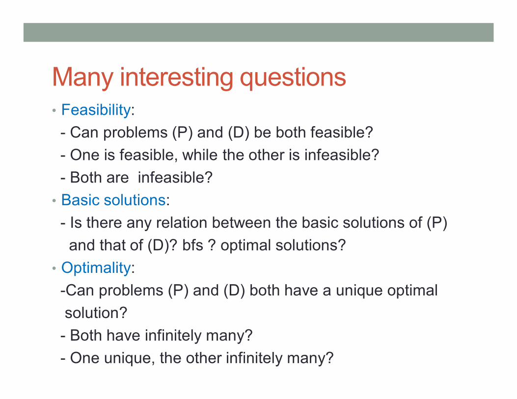
Many interesting questions• Feasibility:

- Can problems (P) and (D) be both feasible?

- One is feasible, while the other is infeasible?

- Both are infeasible?

• Basic solutions:

- Is there any relation between the basic solutions of (P)

and that of (D)? bfs ? optimal solutions?

• Optimality:

-Can problems (P) and (D) both have a unique optimal

solution?

- Both have infinitely many?

- One unique, the other infinitely many?

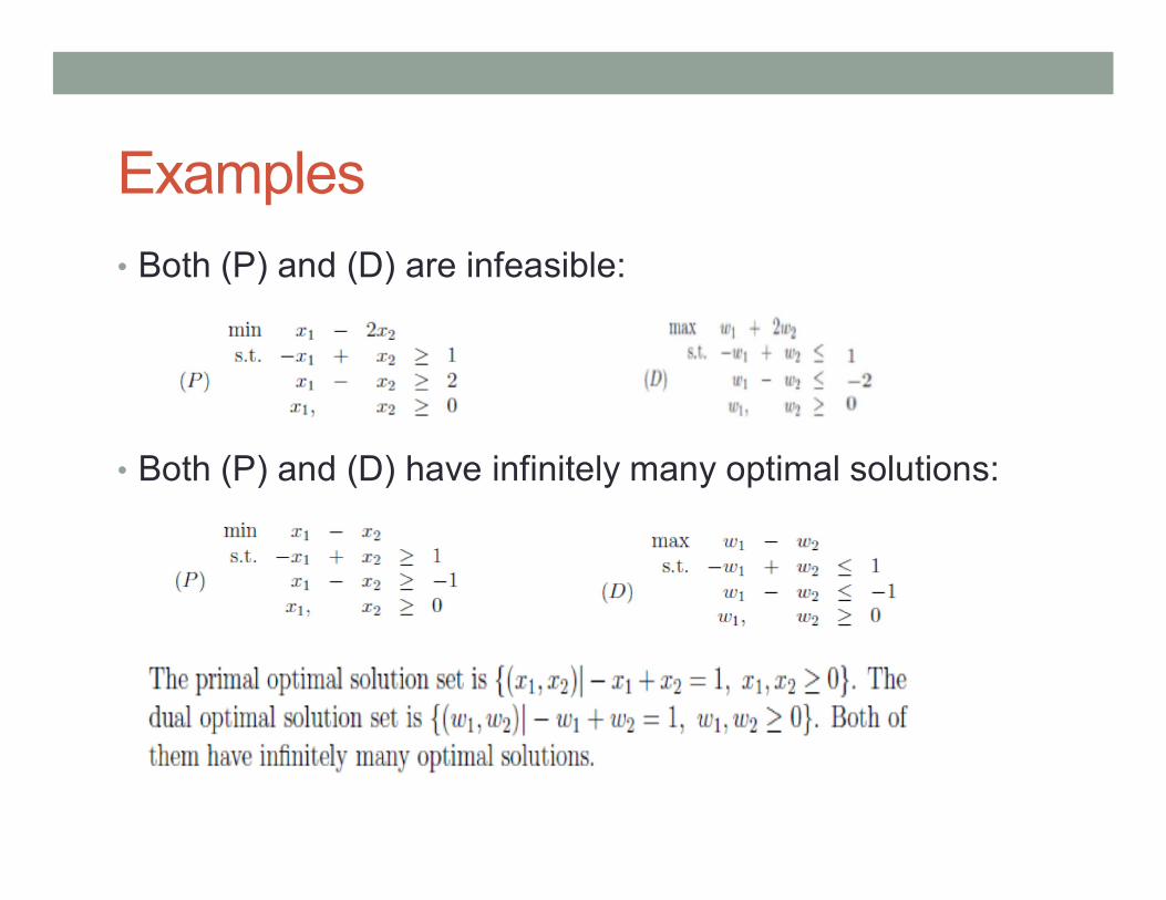
Examples

• Both (P) and (D) are infeasible:

• Both (P) and (D) have infinitely many optimal solutions:

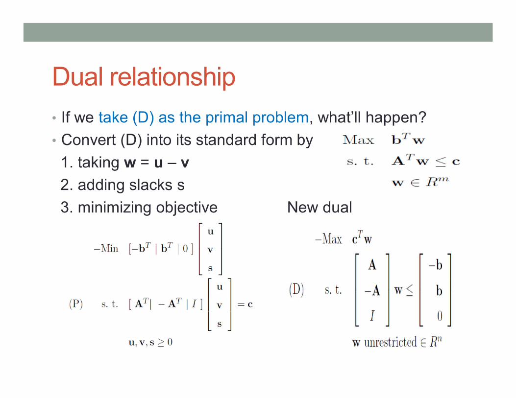
Dual relationship

• If we take (D) as the primal problem, what’ll happen?

• Convert (D) into its standard form by

1. taking w = u – v

2. adding slacks s

3. minimizing objective New dual

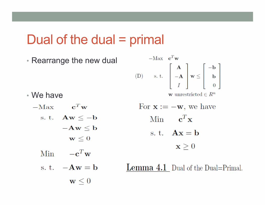
Dual of the dual = primal

• Rearrange the new dual

• We have

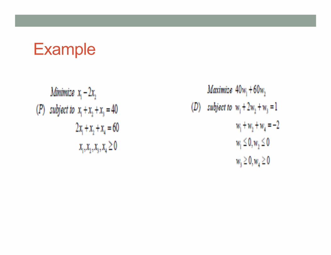
Example

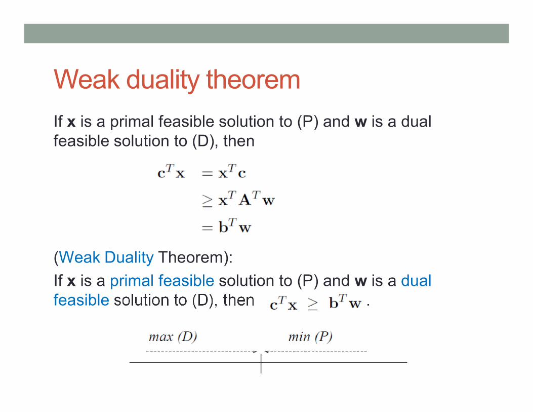
Weak duality theorem

If x is a primal feasible solution to (P) and w is a dual feasible solution to (D), then

(Weak Duality Theorem):

If x is a primal feasible solution to (P) and w is a dual feasible solution to (D), then .

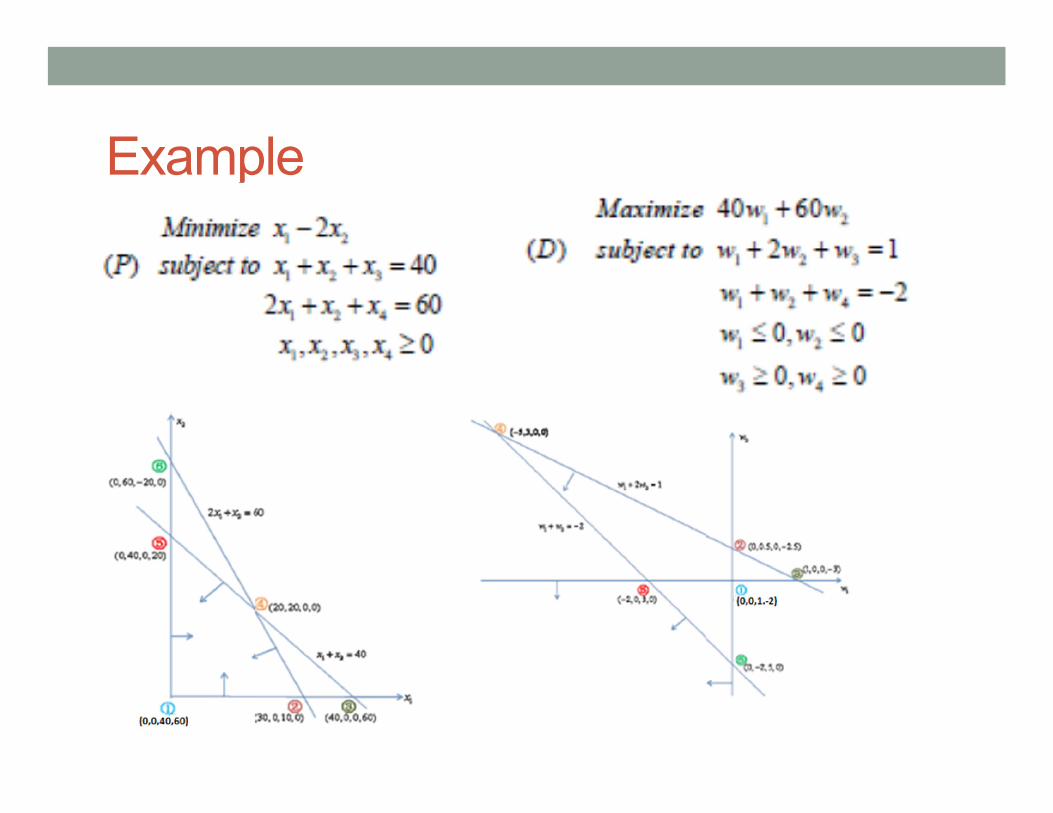
Example

Corollaries

1. If x is primal feasible, w is dual feasible, and

then x is primal optimal, and w is dual optimal.

2. If the primal is unbounded below, then the dual is

infeasible.

(Is the converse statement true? -- watch for infeasibility)

3. If the dual is unbounded above, then the primal is

infeasible.

(Is the converse statement true?)

Strong duality theorem

• Questions:

- Can the results of weak duality be stronger?

- Is there any gap between the primal optimal value and

the dual optimal value?

• Strong Duality Theorem:

Proof of strong duality theorem

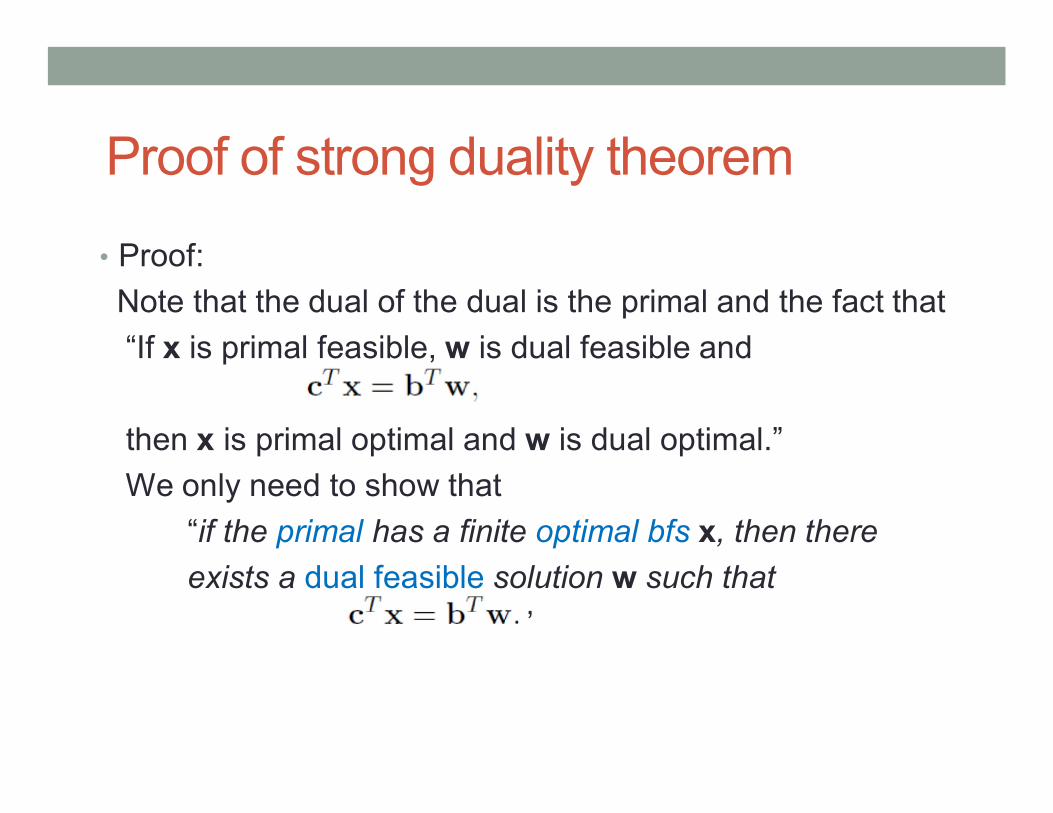
• Proof:

Note that the dual of the dual is the primal and the fact that

“If x is primal feasible, w is dual feasible and

then x is primal optimal and w is dual optimal.”

We only need to show that

“if the primal has a finite optimal bfs x, then there

exists a dual feasible solution w such that

‘’’

Proof - continue

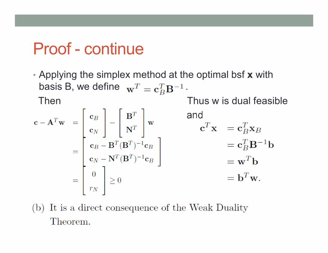
• Applying the simplex method at the optimal bsf x with basis B, we define .

Then Thus w is dual feasible

and

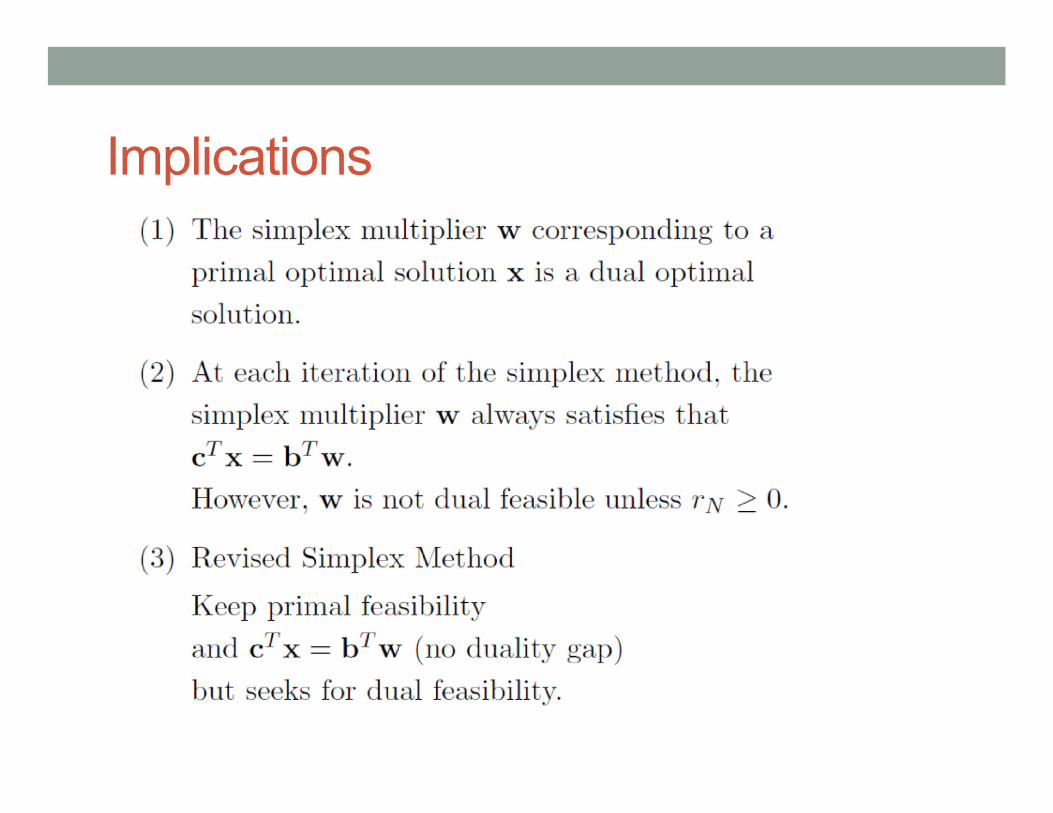
Implications

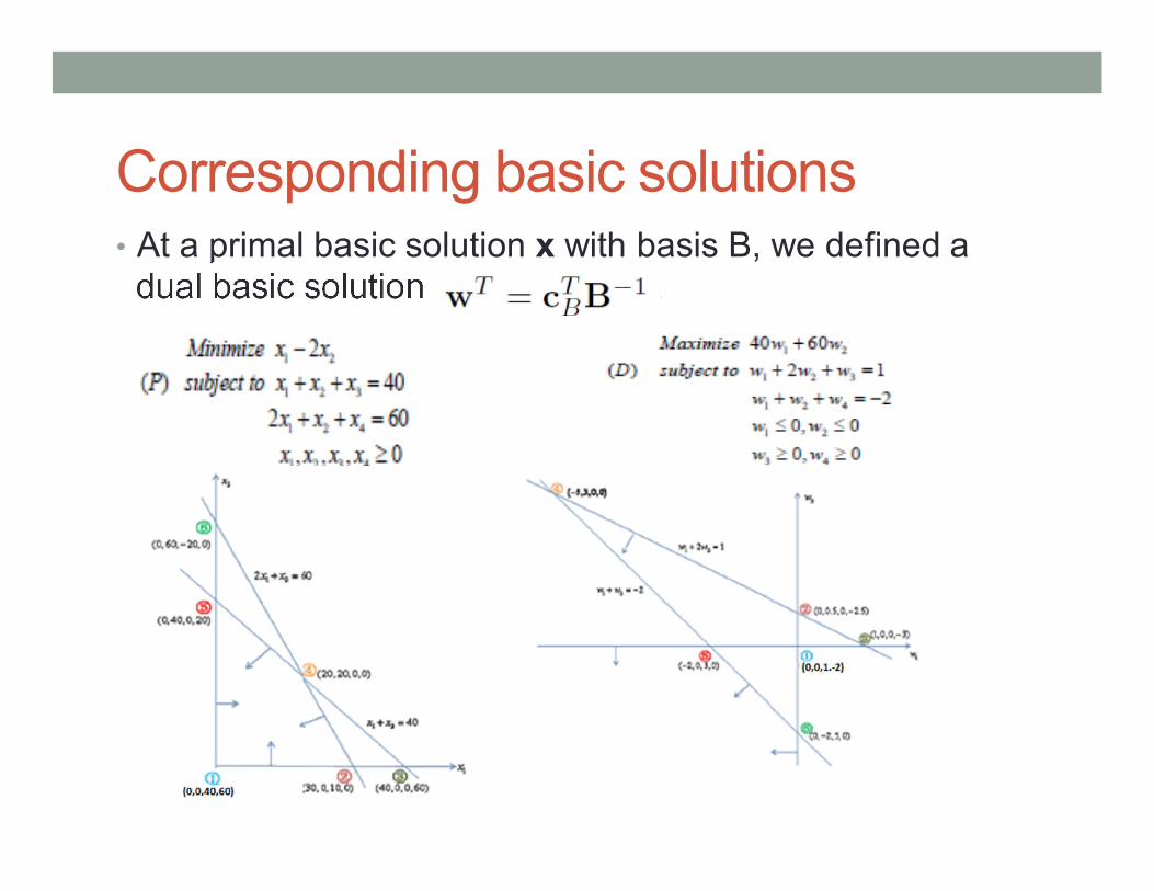
Corresponding basic solutions• At a primal basic solution x with basis B, we defined a

dual basic solution .

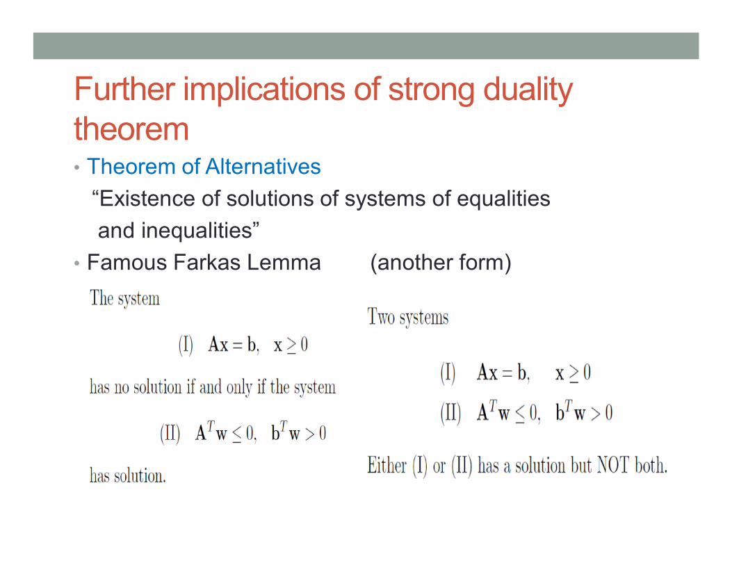
Further implications of strong duality theorem• Theorem of Alternatives

“Existence of solutions of systems of equalities

and inequalities”

• Famous Farkas Lemma (another form)

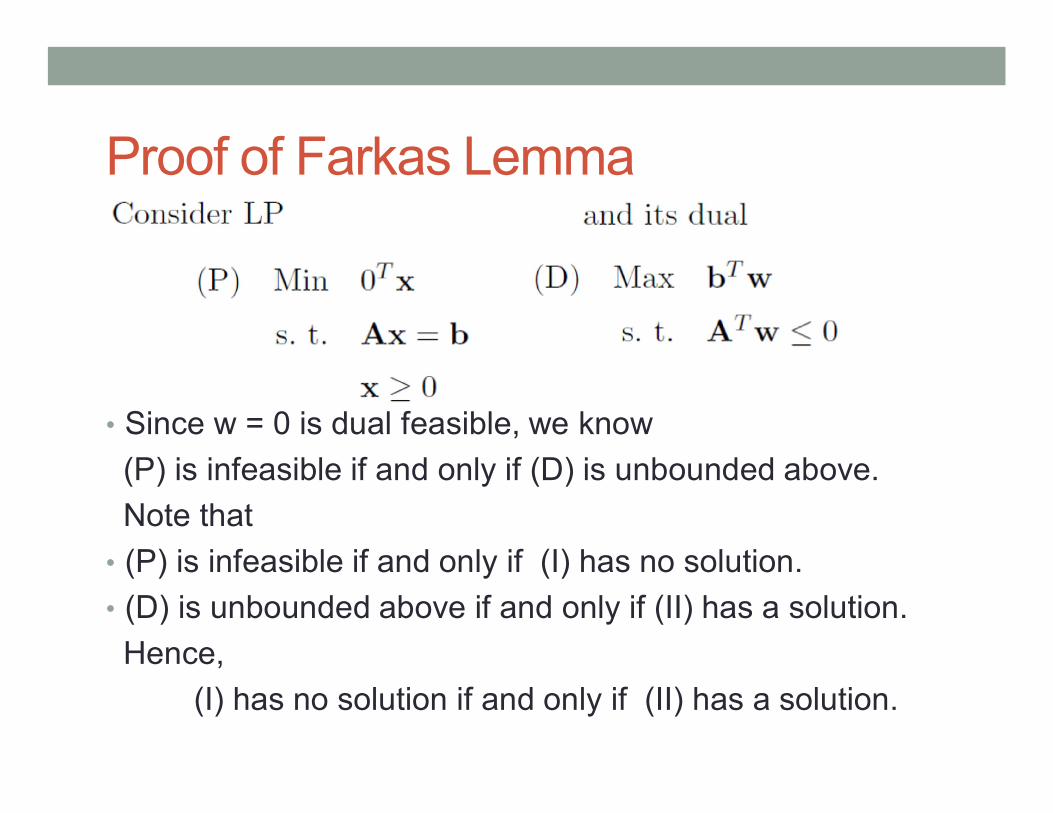
Proof of Farkas Lemma

• Since w = 0 is dual feasible, we know

(P) is infeasible if and only if (D) is unbounded above.

Note that

• (P) is infeasible if and only if (I) has no solution.

• (D) is unbounded above if and only if (II) has a solution.

Hence,

(I) has no solution if and only if (II) has a solution.

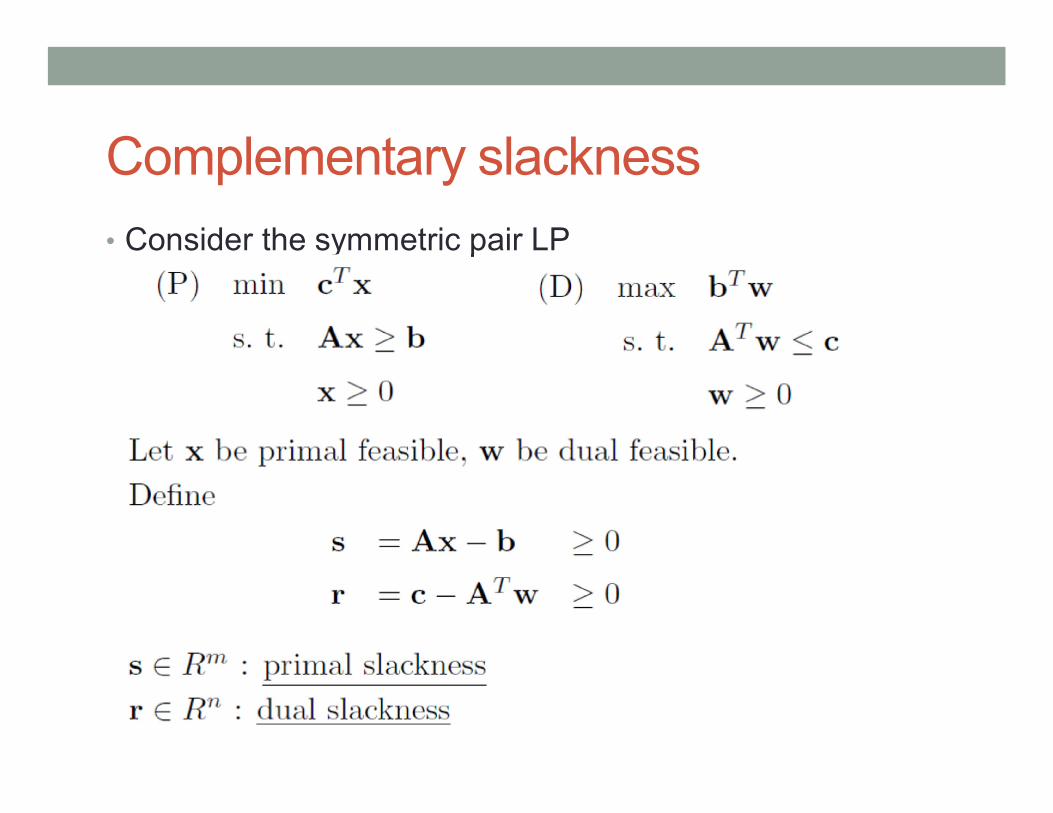
Complementary slackness

• Consider the symmetric pair LP

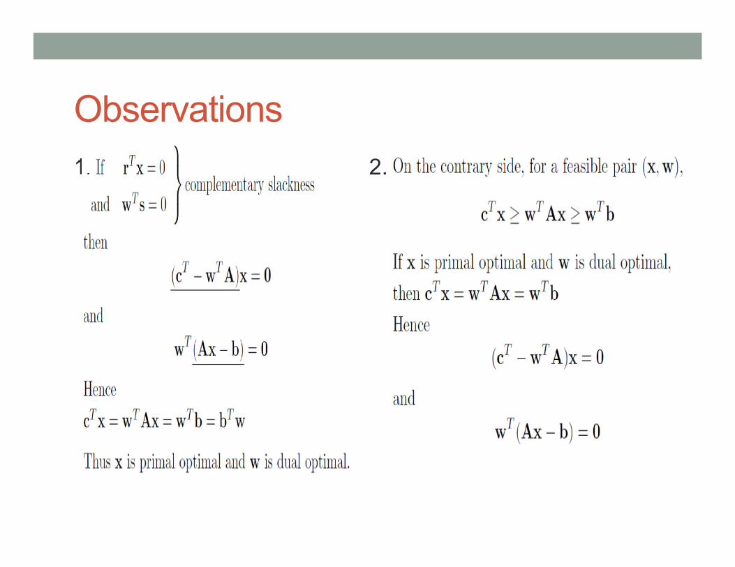
Observations

1. 2.

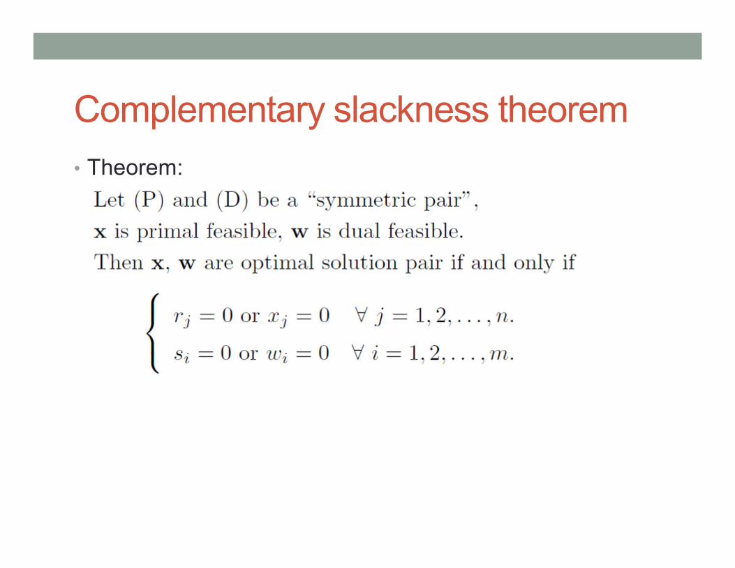
Complementary slackness theorem

• Theorem:

Example

• Consider a relaxed knapsack problem:

• Its dual becomes

4y* > 3 x*1 = 0

7y* > 4 x*2 = 0

10y* = 9 x*3 = ? x*3 = 2 z* = 18

3y* > 2 x*4 = 0

7y* > 5 x*5 = 0

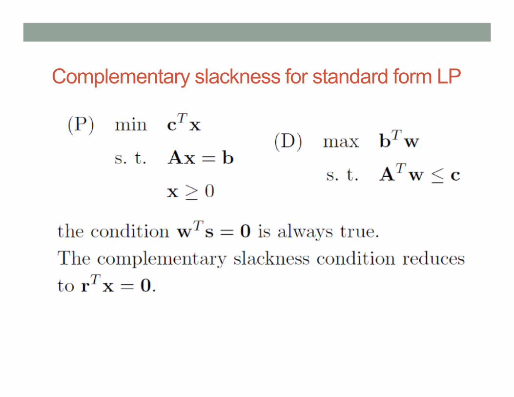
Complementary slackness for standard form LP

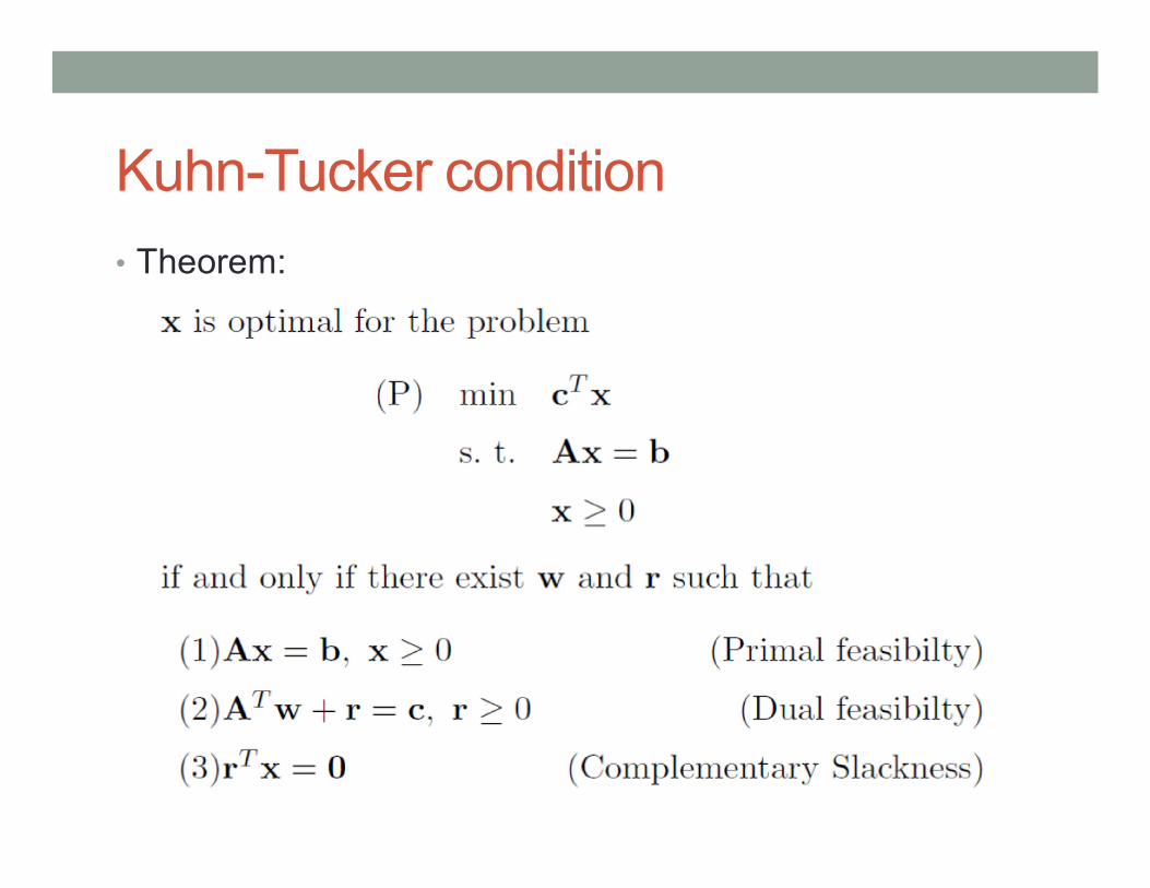
Kuhn-Tucker condition

• Theorem:

Implication

• Solving a linear programming problem is equivalent to

solving a system of linear inequalities.

Economic interpretation of duality

• Is there any special meaning of the dual variables?

• What is a dual problem trying to do?

• What’s the role of the complementary slackness in decision making?

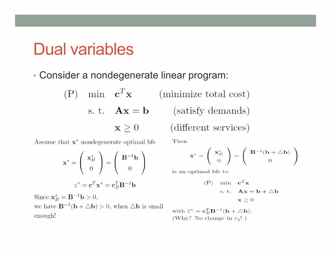
Dual variables

• Consider a nondegenerate linear program:

Dual variable for shadow price

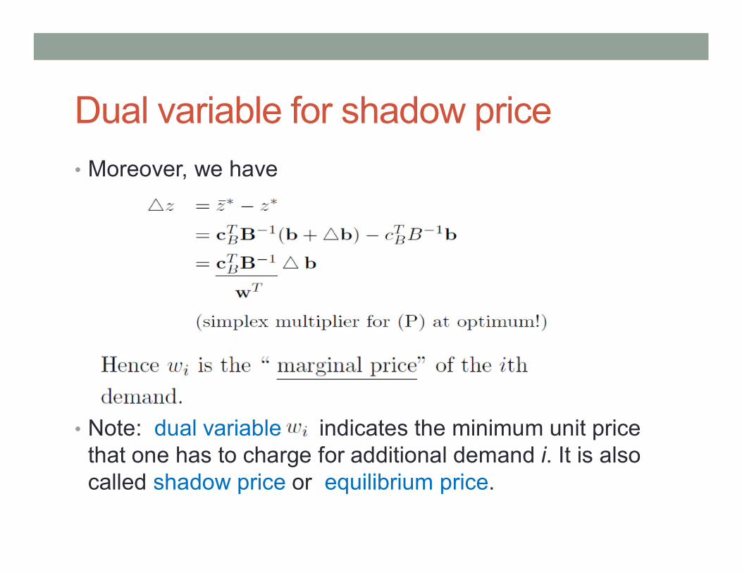
• Moreover, we have

• Note: dual variable indicates the minimum unit price that one has to charge for additional demand i. It is also called shadow price or equilibrium price.

Dual LP problem

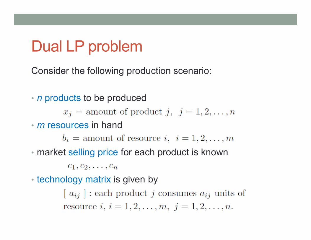
Consider the following production scenario:

• n products to be produced

• m resources in hand

• market selling price for each product is known

• technology matrix is given by

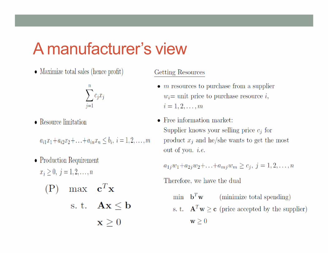
A manufacturer’s view

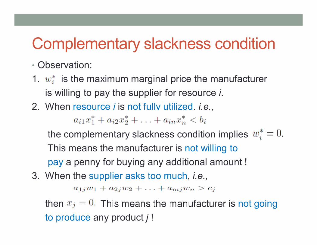
Complementary slackness condition• Observation:

1. is the maximum marginal price the manufacturer

is willing to pay the supplier for resource i.

2. When resource i is not fully utilized, i.e.,

the complementary slackness condition implies

This means the manufacturer is not willing to

pay a penny for buying any additional amount !

3. When the supplier asks too much, i.e.,

then This means the manufacturer is not going

to produce any product j !

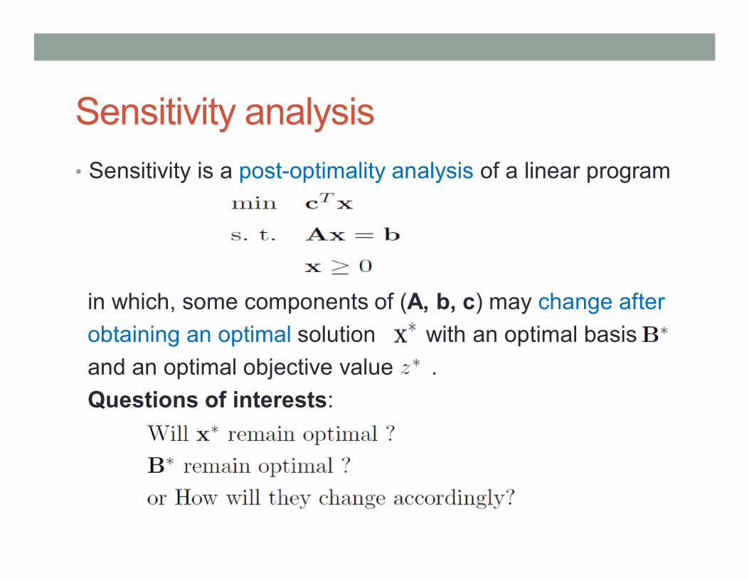
Sensitivity analysis

• Sensitivity is a post-optimality analysis of a linear program

in which, some components of (A, b, c) may change after

obtaining an optimal solution with an optimal basis

and an optimal objective value .

Questions of interests:

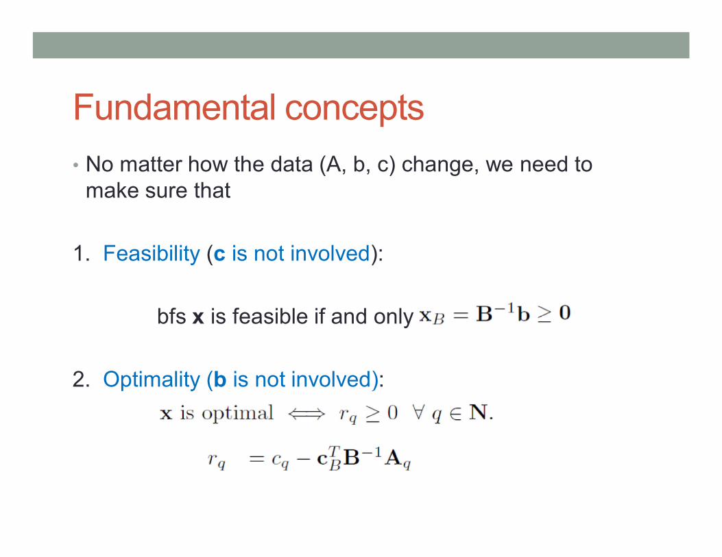
Fundamental concepts

• No matter how the data (A, b, c) change, we need to make sure that

1. Feasibility (c is not involved):

bfs x is feasible if and only if

2. Optimality (b is not involved):

Change in the cost vector

• Scenario:

Consider

• Question:

Within which range of the current optimal

solution remains to be optimal?

Note: when c’ = (0,,0,1,0, …0), we have the regular

sensitivity analysis on each cost coefficient.

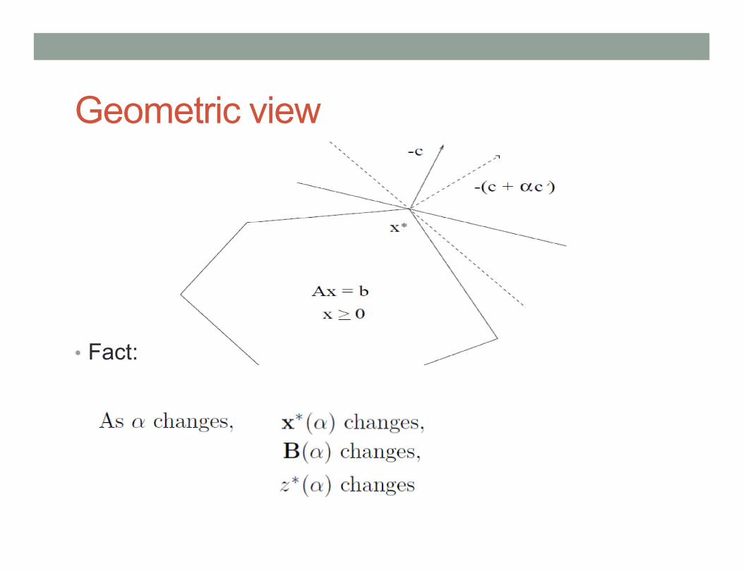
Geometric view

• Fact:

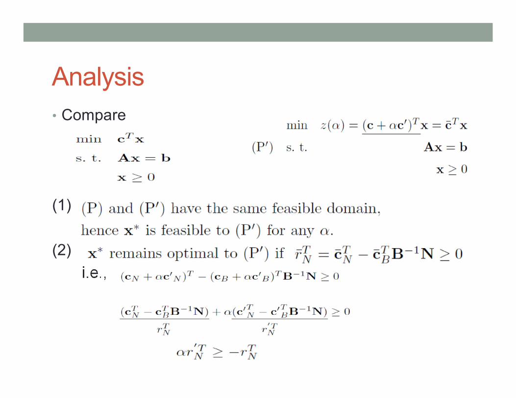
Analysis

• Compare

(1)

(2)

i.e.,

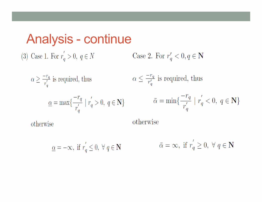
Analysis - continue

Analysis - continue

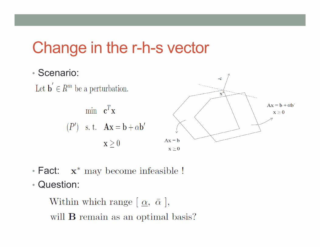
Change in the r-h-s vector

• Scenario:

• Fact:

• Question:

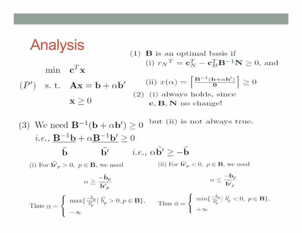
Analysis

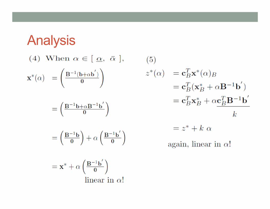
Analysis

Changes in the constraint matrix

• Since both feasibility and optimality are involved, a general analysis is difficult.

• We only consider simple cases such as adding a new variable, removing a variable, adding a new constraint.

Adding a new variable

• Why? A new product, service or activity is introduced.

• Analysis:

Removing a variable

• Why? An activity is no longer available.

Adding a new constraint

• Why? A new restriction is enforces.

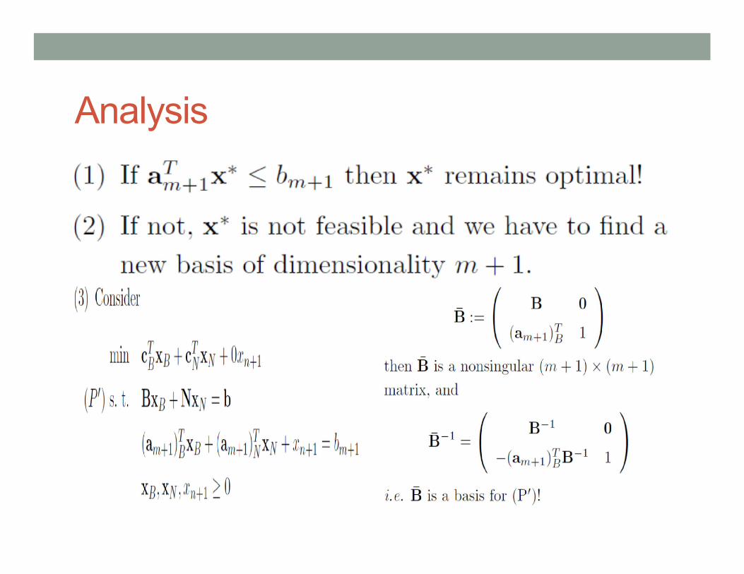
Analysis

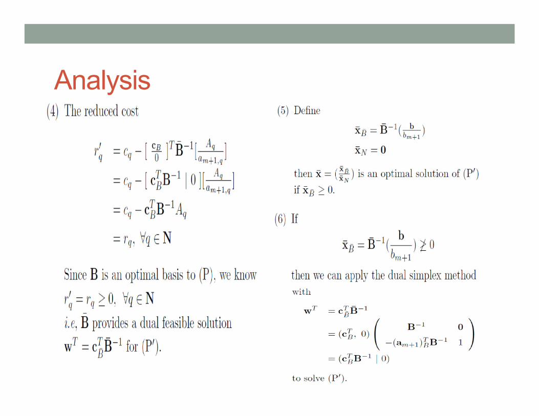
Analysis

Dual simplex method

• What’s the dual simplex method?

- It is a simplex based algorithm that works on the

dual problem directly. In other words, it hops from

one vertex to another vertex along some edge directions

in the dual space.

• It keeps dual feasibility and complementary slackness, butseeks primal feasibility.

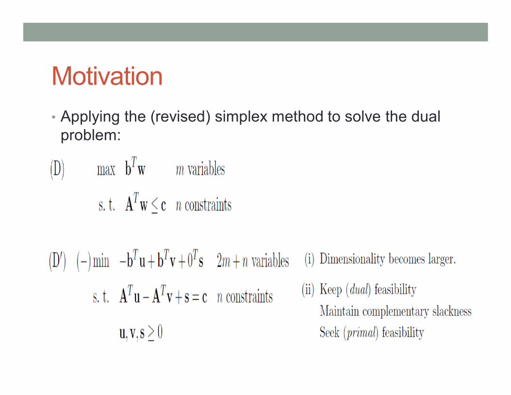
Motivation

• Applying the (revised) simplex method to solve the dual problem:

• At a primal basic solution x with basis B, we defined a dual basic solution .

Corresponding basic solutions

Basic ideas of dual simplex method

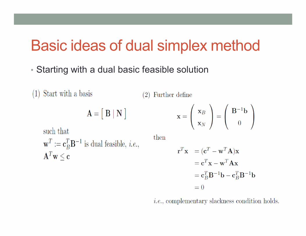
• Starting with a dual basic feasible solution

Basic ideas of dual simplex method

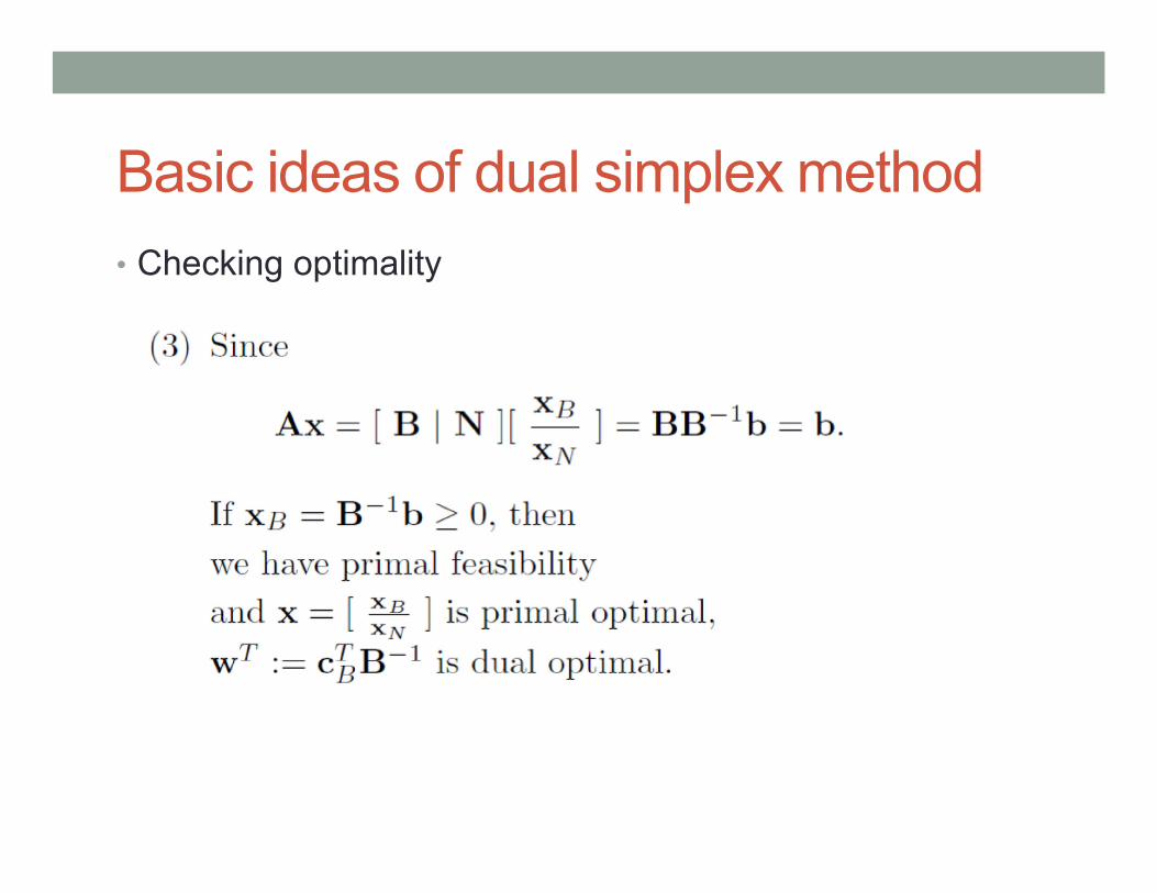
• Checking optimality

Basic ideas of dual simplex method

• Pivoting move

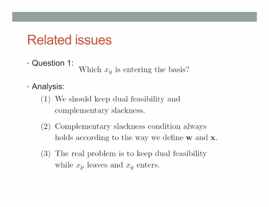
Related issues

• Question 1:

• Analysis:

Related issues

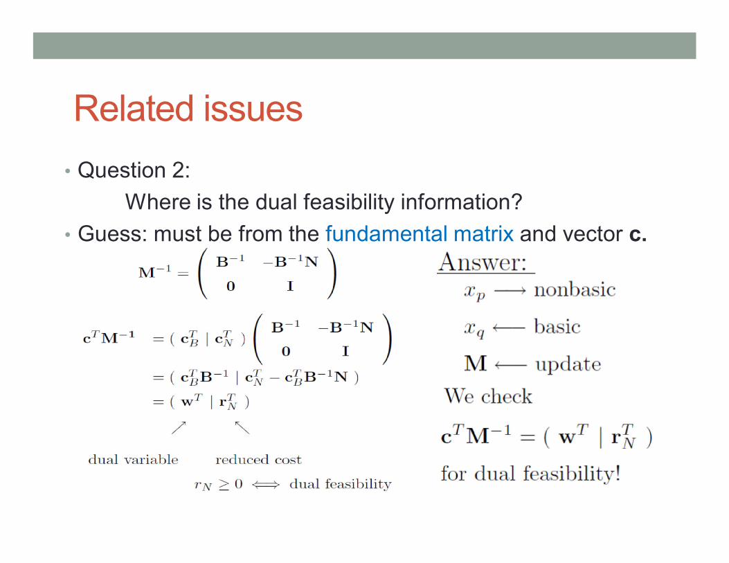
• Question 2:

Where is the dual feasibility information?

• Guess: must be from the fundamental matrix and vector c.

Related issues

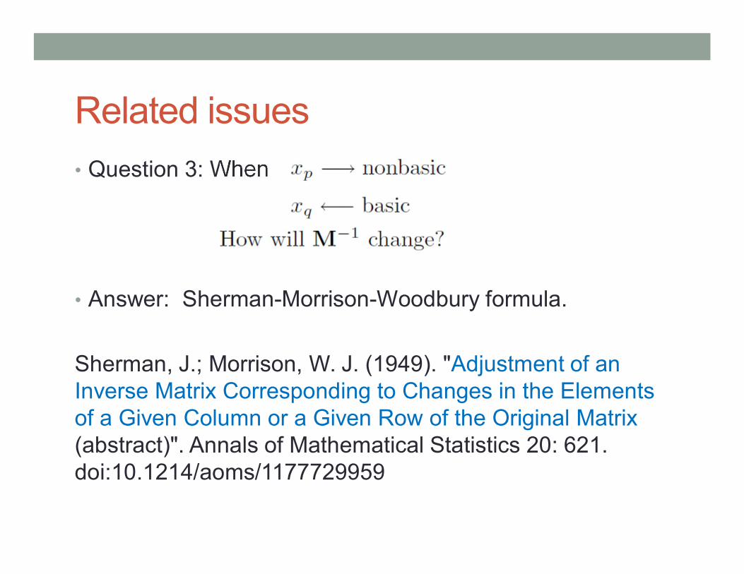
• Question 3: When

• Answer: Sherman-Morrison-Woodbury formula.

Sherman, J.; Morrison, W. J. (1949). "Adjustment of an Inverse Matrix Corresponding to Changes in the Elements of a Given Column or a Given Row of the Original Matrix(abstract)". Annals of Mathematical Statistics 20: 621. doi:10.1214/aoms/1177729959

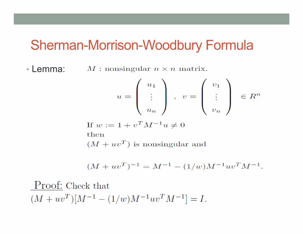
Sherman-Morrison-Woodbury Formula

• Lemma:

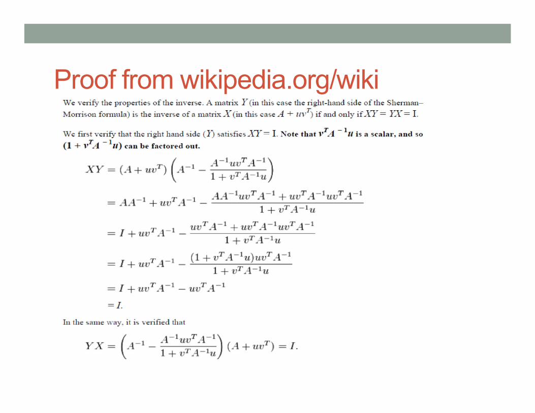
Proof from wikipedia.org/wiki

Observations

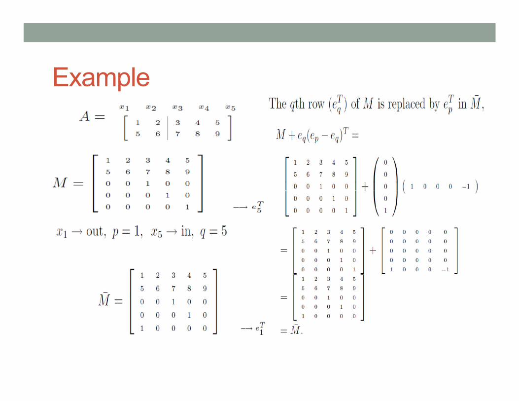
Example

Analysis

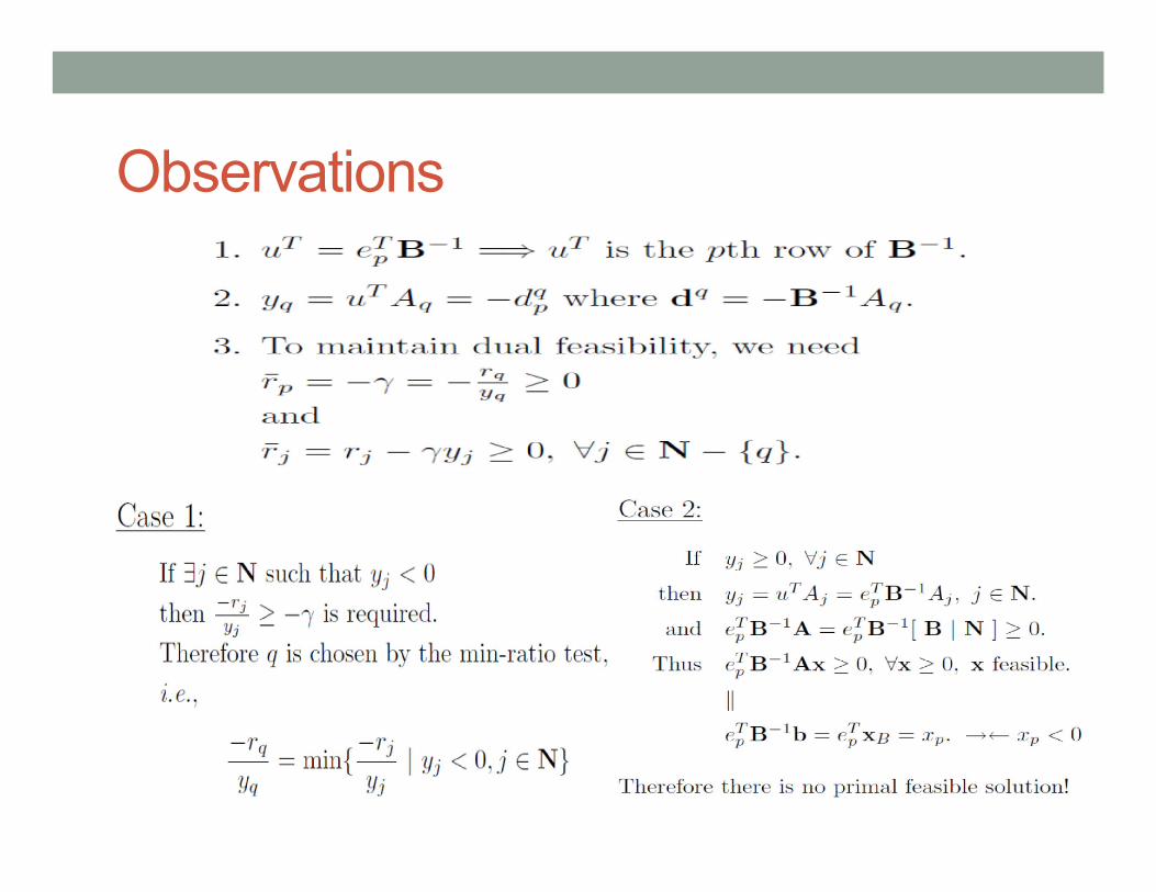
Observations

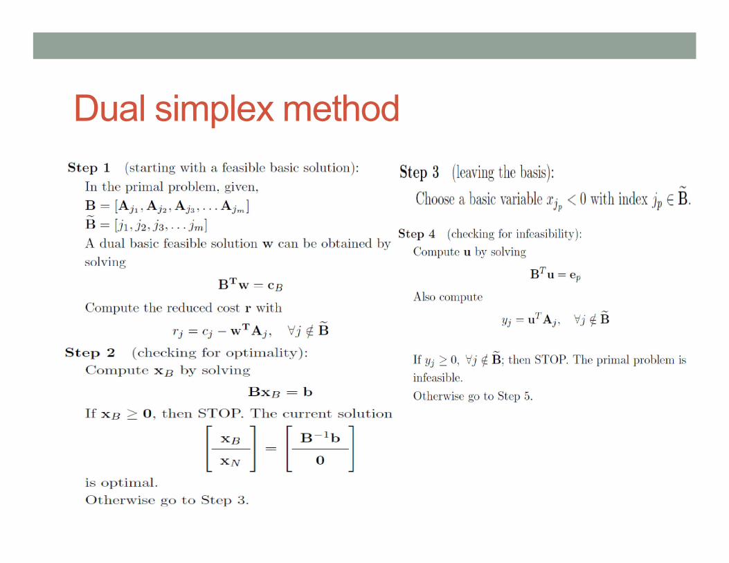
Dual simplex method

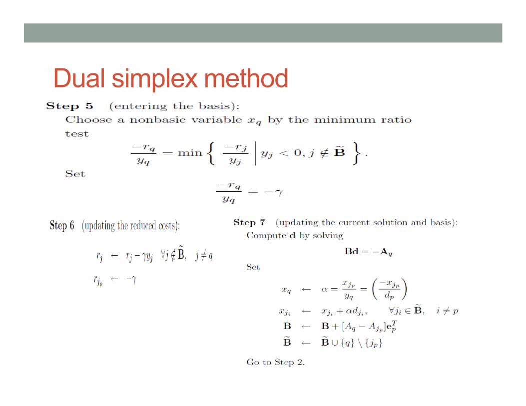
Dual simplex method

Example

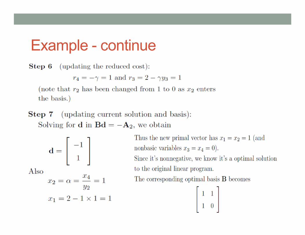
Example - continue

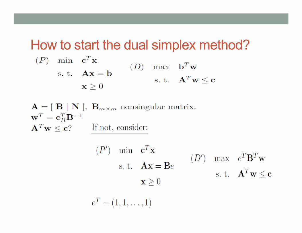
How to start the dual simplex method?

Observations

Remarks

(1) Solving a standard form LP by the dual simplex method

is mathematically equivalent to solving its dual LP

by the revised (primal) simplex method.

(2) The work of solving an LP by the dual simplex method

is about the same as of by the revised (primal)

simplex method.

(3) The dual simplex method is useful for the

sensitivity analysis.

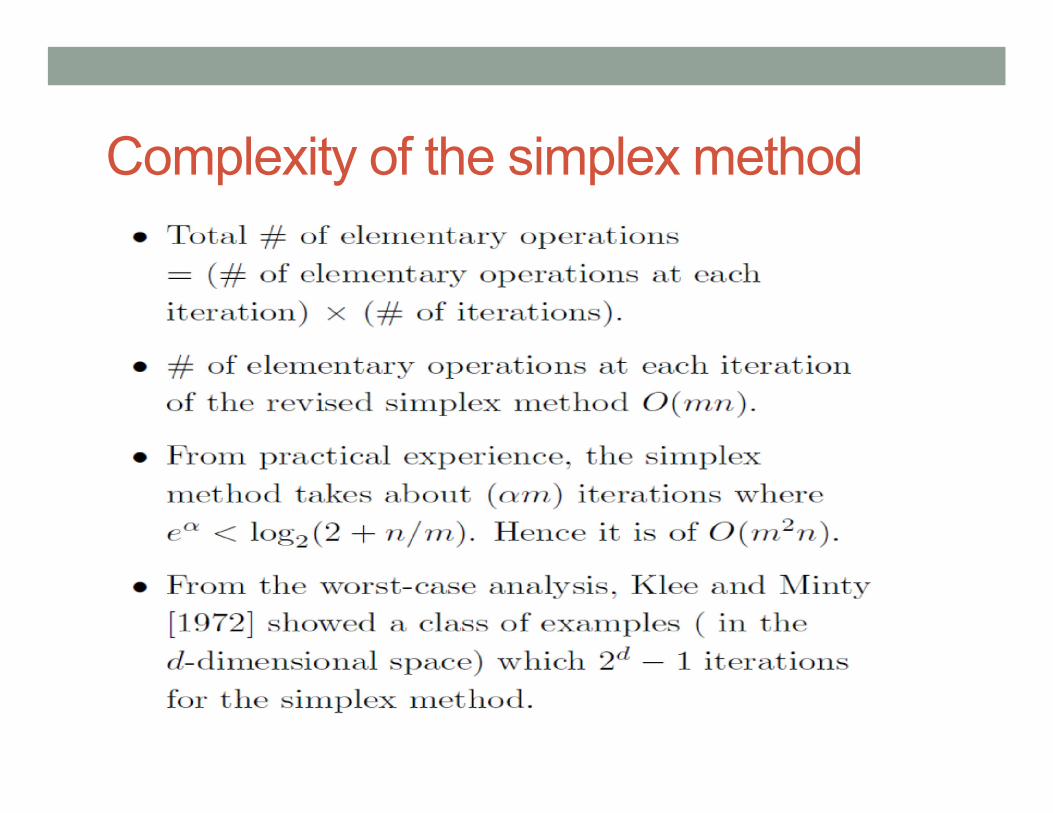
Complexity of the simplex method

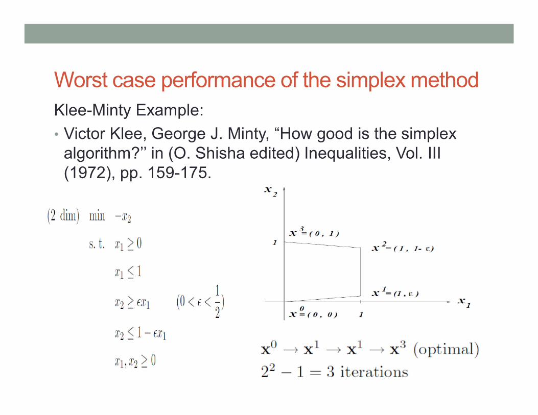
Worst case performance of the simplex method

Klee-Minty Example:

• Victor Klee, George J. Minty, “How good is the simplex algorithm?’’ in (O. Shisha edited) Inequalities, Vol. III (1972), pp. 159-175.

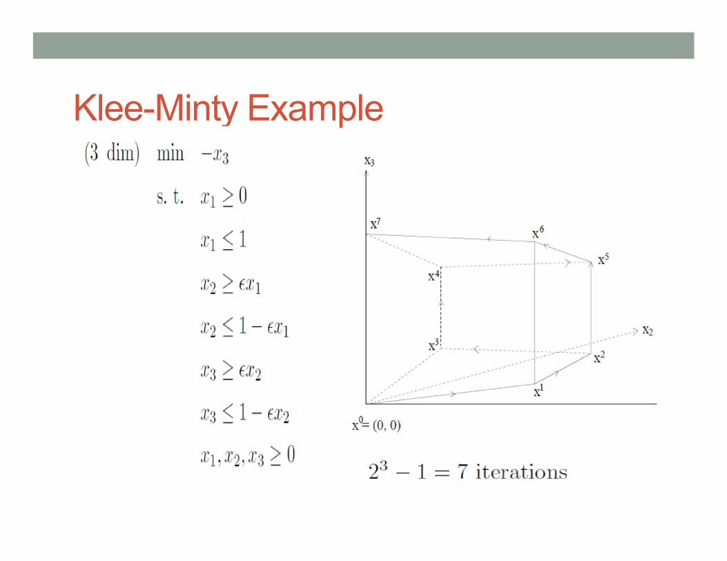
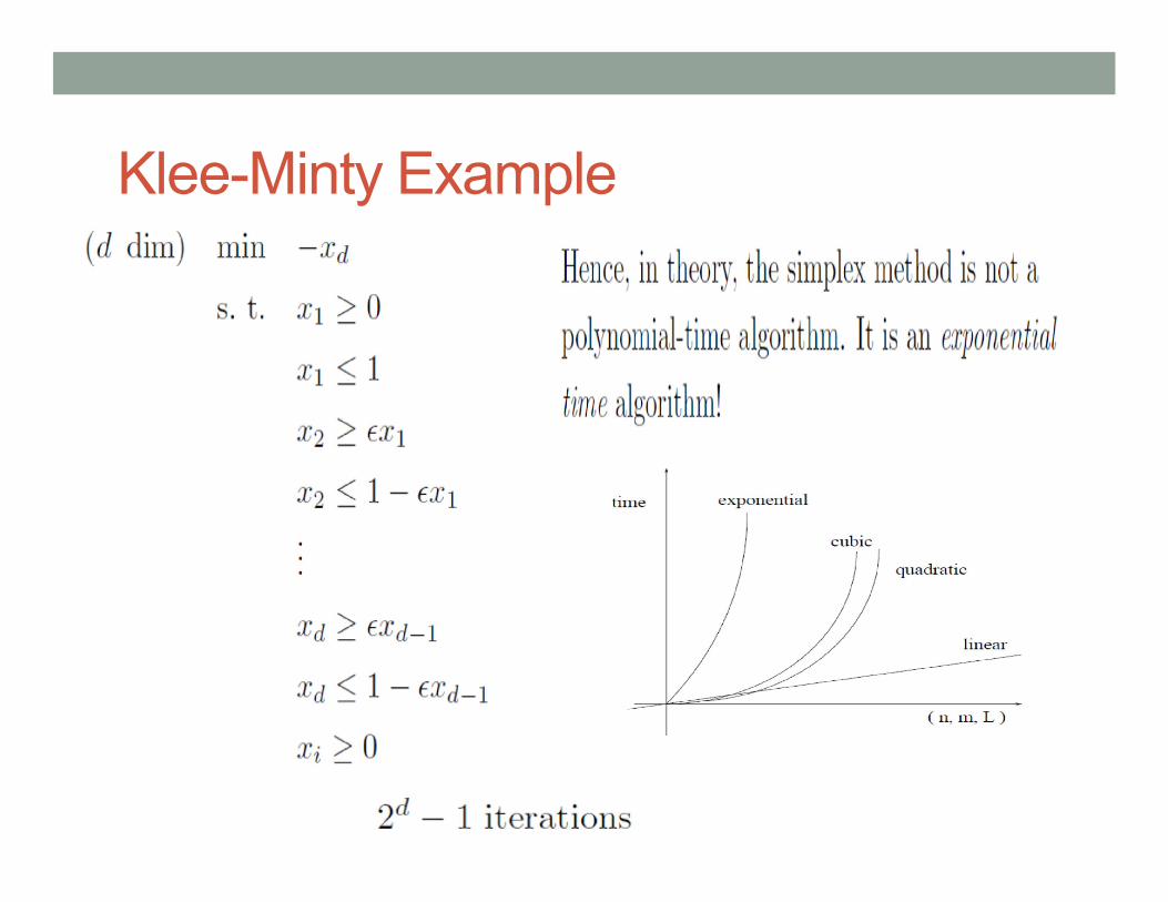
Klee-Minty Example

Klee-Minty Example