lecture 5 intertemporal choice

Intertemporal choiceLecture 5 – Tom Holden

Intermediate Microeconomics Semester 2

http://micro2.tholden.org/

ECO 2051 – Intermediate Microeconomics 1

http://micro2.tholden.org/

Objectives for this topic

• To understand and use (net) present values.

• To appreciate the budget constraint that individuals face when choosing between consumption over time.

• To show how choices are affected by individuals’ preferences between consumption today and tomorrow.

• To relate this analysis to borrowing and saving behaviour.


Readings

• Varian, Chapter 10

• MKR, Chapter 5


Thinking about intertemporal choice

• Intertemporal choice: choice over levels of consumption over time.

• E.g.:

• Given people usually receive income in monthly “lumps”, how should the income be spread over the following month?

• How much should we save for retirement?

• Is it rational to take out student loans?

• When should firms invest in a project that pays off in the future?


Think about your intertemporal choices

• Did you save before you came to university?

• Are you borrowing?

• At what rate of interest?

• Does your borrowing change depending on the rate of interest you face?

• To what extent do you think about your future income when making these decisions?

• Do you think your consumption decisions will change if you get a definite job/placement offer?


Present and future values

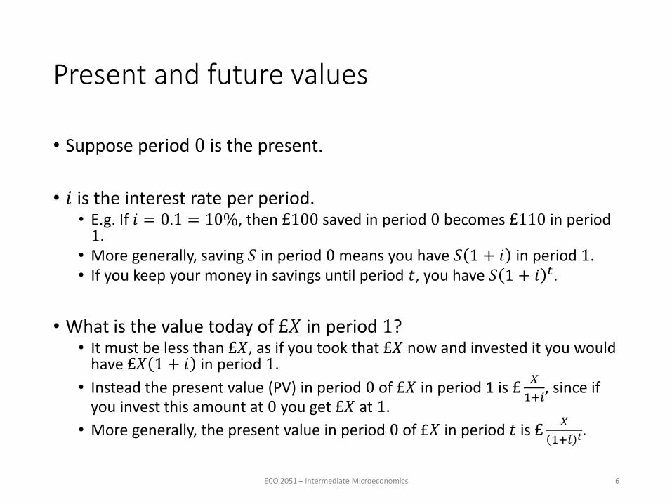
• Suppose period 0 is the present.

• 𝑖 is the interest rate per period.• E.g. If 𝑖 = 0.1 = 10%, then £100 saved in period 0 becomes £110 in period 1.

• More generally, saving 𝑆 in period 0means you have 𝑆 1 + 𝑖 in period 1.• If you keep your money in savings until period 𝑡, you have 𝑆 1 + 𝑖 𝑡.

• What is the value today of £𝑋 in period 1?• It must be less than £𝑋, as if you took that £𝑋 now and invested it you would

have £𝑋 1 + 𝑖 in period 1.

• Instead the present value (PV) in period 0 of £𝑋 in period 1 is £𝑋

1+𝑖, since if

you invest this amount at 0 you get £𝑋 at 1.

• More generally, the present value in period 0 of £𝑋 in period 𝑡 is £𝑋

1+𝑖 𝑡.


Example present values

• Present values reduce quite fast as we look further into the future under reasonable interest rates.


Rate 𝒕 = 𝟏 𝒕 = 𝟐 𝒕 = 𝟓 𝒕 = 𝟏𝟎 𝒕 = 𝟏𝟓 𝒕 = 𝟐𝟎 𝒕 = 25 𝒕 = 30

0.05 .95 .91 .78 .61 .48 .37 .30 .23

0.10 .91 .83 .62 .39 .39 .15 .09 .06

0.15 .87 .76 .50 .25 .25 .06 .03 .02

0.20 .83 .69 .40 .16 .16 .03 .01 .00

Value of £𝟏 𝒕 years in the future under different interest rates

More complicated present values

• Suppose you believe buying a share in a company (in period 0) would give you a stream of dividends given by 𝑑1, 𝑑2, … where 𝑑𝑡 is the dividend you get in period 𝑡.

• What is the present value of this dividend stream?

• It is the PV of getting 𝑑1 in period 1 plus the PV of getting 𝑑2 in period 2, plus…

• I.e. 𝑑1

1+𝑖 1+𝑑2

1+𝑖 2+⋯ = 𝑡=1

∞ 𝑑𝑡

1+𝑖 𝑡

• So at what price should you be prepared to buy the share? What should you do if you couldn’t afford it at this price?

• Note that high interest rates reduce present values.


More on present value (1/4)

• Suppose a consumer’s income stream is currently given by 𝑦0, 𝑦1, 𝑦2, … where 𝑦𝑡 is their income at 𝑡, and period 0 is the present.

• If they are offered the chance to switch to an alternative stream 𝑧0, 𝑧1, 𝑧2, … should they take it?

• Could be a new job, or a degree, or an investment.

• PV of the original stream, 𝑣𝑦 is 𝑣𝑦 = 𝑦0 +𝑦1

1+𝑖+𝑦2

1+𝑖 2+⋯ = 𝑡=0

∞ 𝑦𝑡

1+𝑖 𝑡.

• PV of the alternative stream, 𝑣𝑧 is 𝑣𝑧 = 𝑧0 +𝑧1

1+𝑖+𝑧2

1+𝑖 2+⋯ = 𝑡=0

∞ 𝑧𝑡

1+𝑖 𝑡.



• Suppose that 𝑣𝑧 > 𝑣𝑦 and they do take the 𝑧𝑡 stream.

• Then, by going to the bank they can borrow 𝑧1

1+𝑖against their period 1

income. (When period 1 arrives they will have to repay 𝑧1

1+𝑖1 + 𝑖 = 𝑧1,

which is their period 1 income.) And 𝑧2

1+𝑖 2against period 2 income, etc etc.

• So they can borrow 𝑡=1∞ 𝑧𝑡

1+𝑖 𝑡= 𝑣𝑧 − 𝑧0 in total (note sum starts at 1), so if

they wanted to they could spend 𝑣𝑧 in period 0 and starve from then on.

• Suppose they borrow all of this money, then immediately put a total of 𝑡=1∞ 𝑦𝑡

1+𝑖 𝑡= 𝑣𝑦 − 𝑦0 into their saving account, leaving 𝑣𝑧 − 𝑣𝑦 − 𝑦0 =

𝑣𝑧 − 𝑣𝑦 + 𝑦0 in their pocket.



• As 𝑣𝑧 − 𝑣𝑦 > 0, this enables them to spend more than 𝑦0 in the first period.

• The next period thanks to interest they now have 1 + 𝑖 𝑡=1∞ 𝑦𝑡

1+𝑖 𝑡= 𝑦1 +

𝑡=2∞ 𝑦𝑡

1+𝑖 𝑡−1in the bank.

• If they spend 𝑦1 they still have 𝑡=2∞ 𝑦𝑡

1+𝑖 𝑡−1in savings.

• The period after this has become 1 + 𝑖 𝑡=2∞ 𝑦𝑡

1+𝑖 𝑡−1= 𝑦2 + 𝑡=3

∞ 𝑦𝑡

1+𝑖 𝑡−2.

• Continuing in this way, the consumer may spend 𝑦𝑡 in every period after 0.



• But they spent more in 0, thus consumption is higher in one period, and the same in all others, so the consumer must be better-off overall, as long as their preferences are strictly increasing.

• So when 𝑣𝑧 > 𝑣𝑦 the consumer is strictly better off taking the 𝑧𝑡stream, independent of preferences.

• As Varian says:• “Present value is the only correct way to convert a stream of payments into

today’s dollars… If a consumer can freely borrow and lend at a constant rate of interest, then the consumer will always prefer a pattern of income with a higher present value to a pattern with a lower present value.”


PV examples: Comparing two simple income streams

• Investment A pays £100 now and £200 next year.

• Investment B pays £0 now and £310 next year.

• With a zero interest rate we just add up the payments £310 > £300 so investment B is better.

• But with a sufficiently high interest rate investment A is preferred.

• For example if 𝑖 = 0.2 then PV𝐴 = 100 +200

1.2= 266.67 & PV𝐵 = 0 +

310

1.2=

258.33.

• The fact that A pays more money earlier on means that it will have a higher present value if the interest rate is high enough.


PV examples: Perpetuities

• Buying a perpetuity guarantees the holder of the perpetuity to a payment of 𝑑 in all future periods. What is the PV of such a perpetuity?

• Using the formula from earlier, the present value of the perpetuity, 𝑣,

satisfies 𝑣 = 𝑡=1∞ 𝑑

1+𝑖 𝑡=𝑑

1+𝑖+𝑑

1+𝑖 2+𝑑

1+𝑖 3+⋯.

• Thus 1 + 𝑖 𝑣 = 𝑑 +𝑑

1+𝑖+𝑑

1+𝑖 2+⋯ = 𝑑 + 𝑣

• So 𝑖𝑣 = 𝑑, i.e. 𝑣 =𝑑

𝑖.

• If you invest an amount 𝑣 at an interest rate 𝑖, then you get 𝑖𝑣 each period.


PV examples: Bonds

• Buying a 𝑇-period bond guarantees the holder to:• A payment of 𝑑 in periods 1,2,… , 𝑇 − 1. (This is called “the coupon”.)

• A payment of 𝐹 in period 𝑇. (This is called “the face value”.)

• Thus the present value of the bond, 𝑣, satisfies:

𝑣 =

𝑡=1

𝑇−1𝑑

1 + 𝑖 𝑡+𝐹

1 + 𝑖 𝑇=𝑑

1 + 𝑖+𝑑

1 + 𝑖 2+⋯+

𝑑

1 + 𝑖 𝑇−1+𝐹

1 + 𝑖 𝑇

• Thus:

1 + 𝑖 𝑣 = 𝑑 +𝑑

1 + 𝑖+𝑑

1 + 𝑖 2+⋯+

𝑑

1 + 𝑖 𝑇−2+

𝐹

1 + 𝑖 𝑇−1

= 𝑑 +𝑑

1 + 𝑖+𝑑

1 + 𝑖 2+⋯+

𝑑

1 + 𝑖 𝑇−2+

𝑑

1 + 𝑖 𝑇−1+𝐹

1 + 𝑖 𝑇+𝐹 − 𝑑

1 + 𝑖 𝑇−1−𝐹

1 + 𝑖 𝑇

= 𝑑 + 𝑣 +𝐹 − 𝑑

1 + 𝑖 𝑇−1−𝐹

1 + 𝑖 𝑇

• So 𝑖𝑣 = 𝑑 +𝐹−𝑑

1+𝑖 𝑇−1−𝐹

1+𝑖 𝑇= 𝑑 +

𝑖𝐹− 1+𝑖 𝑑

1+𝑖 𝑇, i.e. 𝑣 =

𝑑

𝑖+𝐹− 1+𝑖

𝑑

𝑖

1+𝑖 𝑇.


PV examples: Investment with maintenance payments

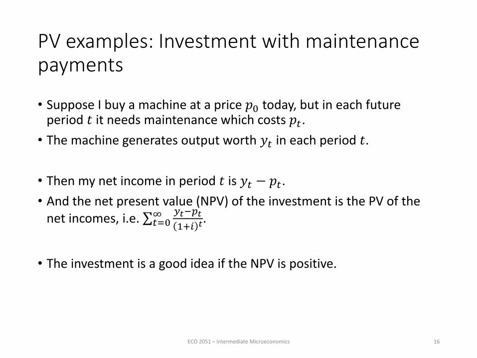
• Suppose I buy a machine at a price 𝑝0 today, but in each future period 𝑡 it needs maintenance which costs 𝑝𝑡.

• The machine generates output worth 𝑦𝑡 in each period 𝑡.

• Then my net income in period 𝑡 is 𝑦𝑡 − 𝑝𝑡.

• And the net present value (NPV) of the investment is the PV of the net incomes, i.e. 𝑡=0

∞ 𝑦𝑡−𝑝𝑡

1+𝑖 𝑡.

• The investment is a good idea if the NPV is positive.


PV examples: Cost benefit analysis

• Cost benefit analysis (CBA) works on exactly the same principles as the investment analysis we have just seen.

• If for some policy the net present value to society is positive, then the policy is worth pursuing.

• But here all the benefits and costs are included, and an attempt is made to value them as those experiencing them would value them (so market prices are not always used if externalities etc. are important).

• 𝑖 is consdered more broadly as the ‘social rate of time preference’.• May differ quite substantially from the interest rate.

• E.g. 𝑖 in Stern report was 2%. Much lower than businesses would use.


PV examples: Intertemporal budget constraints (2 period case)

• 𝐶0 is consumption in period 0, 𝐶1 is consumption in period 1.

• 𝑃0 is the price of the consumption good in period 0, 𝑃1 is its price in period 1.

• 𝑌0 is income in period 0, 𝑌1 is income in period 1.

• The budget constraint says the PV of expenditure must equal the PV of consumption.• I cannot die with debts, and I do not want to leave any assets behind when I die.

• I.e. 𝑃0𝐶0 +𝑃1𝐶1

1+𝑖= 𝑌0 +

𝑌1

1+𝑖.

• Increasing interest rates make next period’s consumption cheaper. (I have to save less today to pay for it).

• Increasing interest rates make next period’s income less valuable. (I can borrow less today using it).


The intertemporal budget constraint


When 𝑃0 = 𝑃1, the slope of the budget constraint is – (1 + 𝑖) for each £1 given up now, we get £ 1 + 𝑖 in future. For each extra £1 consumed now, we give up £ 1 + 𝑖 in future.

𝐼𝑡 is income (i.e. what we were calling 𝑌𝑡.)

Preferences


A person who was totally indifferent between consumption today and in the future would have indifference curves with a slope of −1. People are likely to prefer a mix of consumption in present and future, so ICs are convex.Because impatient individuals prefer to consume today, on the 45° line we need more than £1tomorrow to give up £1 today.Steeper indifference curves imply more impatience.

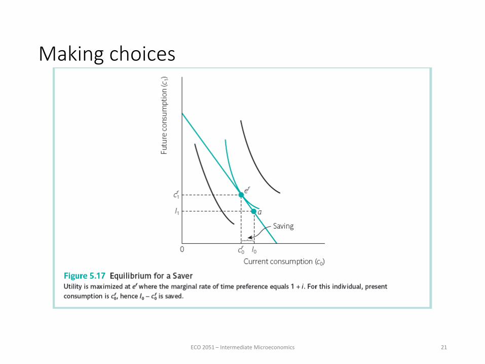
Making choices


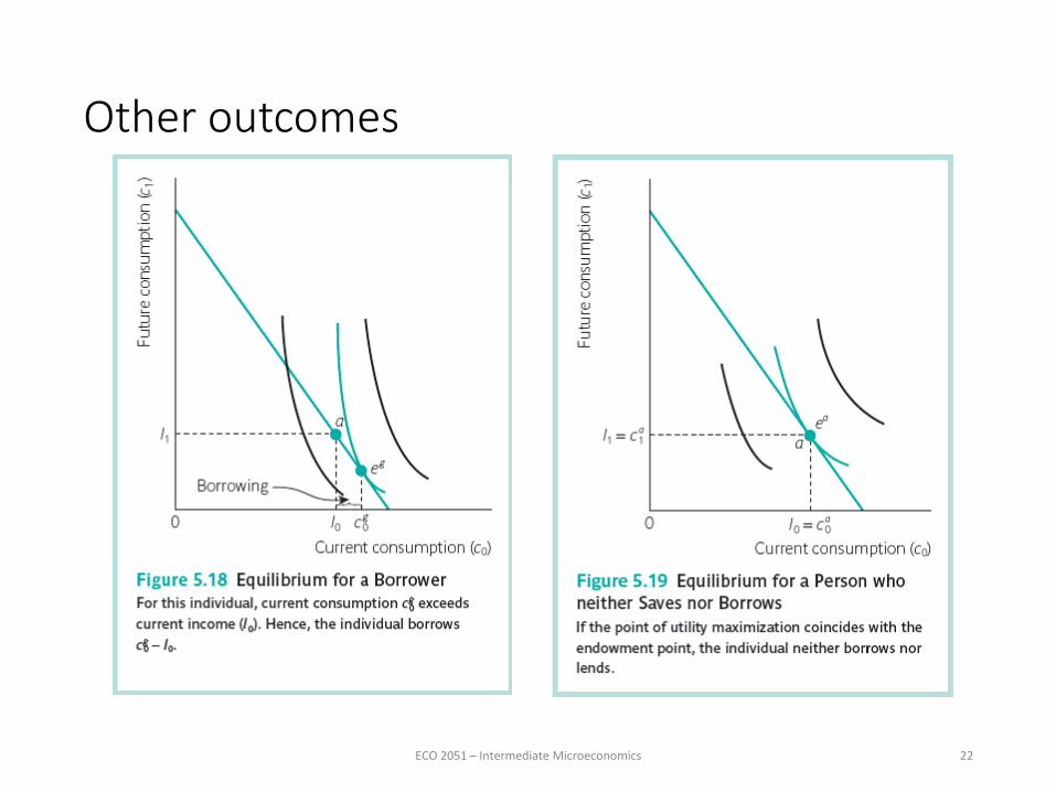
Other outcomes


Example

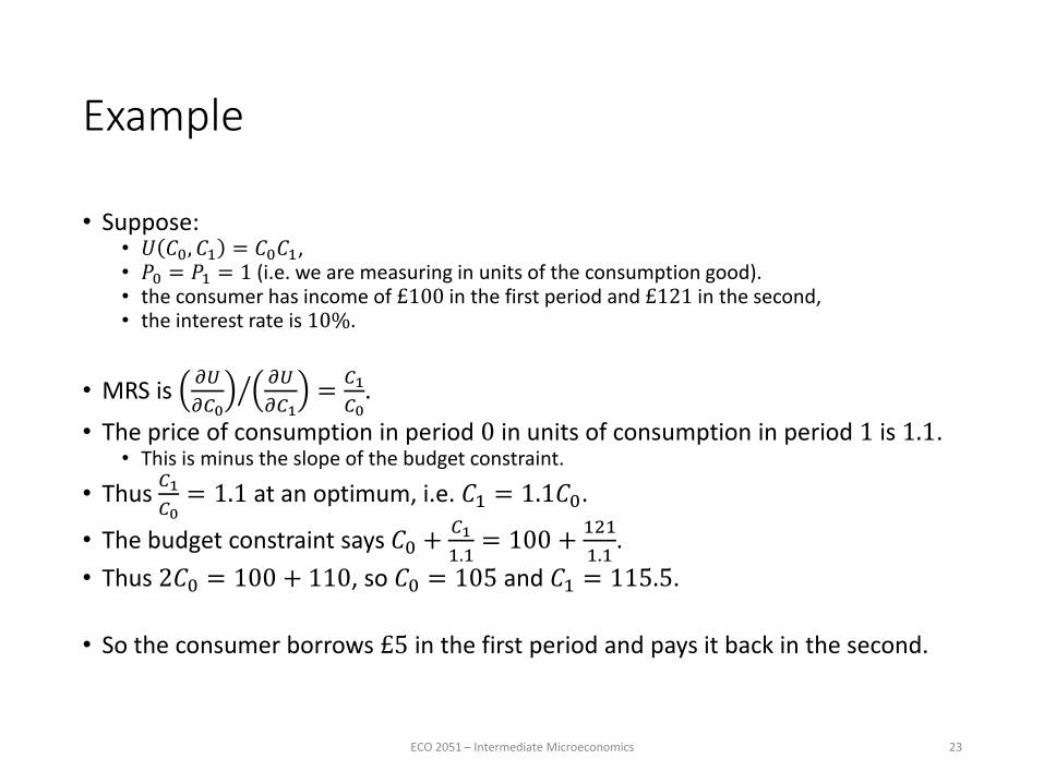
• Suppose:• 𝑈 𝐶0, 𝐶1 = 𝐶0𝐶1,• 𝑃0 = 𝑃1 = 1 (i.e. we are measuring in units of the consumption good).• the consumer has income of £100 in the first period and £121 in the second,• the interest rate is 10%.

• MRS is 𝜕𝑈

𝜕𝐶0

𝜕𝑈

𝜕𝐶1=𝐶1

𝐶0.

• The price of consumption in period 0 in units of consumption in period 1 is 1.1.• This is minus the slope of the budget constraint.

• Thus 𝐶1

𝐶0= 1.1 at an optimum, i.e. 𝐶1 = 1.1𝐶0.

• The budget constraint says 𝐶0 +𝐶1

1.1= 100 +

121

1.1.

• Thus 2𝐶0 = 100 + 110, so 𝐶0 = 105 and 𝐶1 = 115.5.

• So the consumer borrows £5 in the first period and pays it back in the second.


General case (1/2)

• The Lagrangian for the consumer’s optimisation problem is:

ℒ = 𝑈 𝐶0, 𝐶1 − 𝜆 𝑃0𝐶0 +𝑃1𝐶11 + 𝑖− 𝑌0 −

𝑌11 + 𝑖

• FOC 𝐶0: 0 =𝜕𝑈

𝜕𝐶0− 𝜆𝑃0, so 𝜆 =

1

𝑃0

𝜕𝑈

𝜕𝐶0

• FOC 𝐶1: 0 =𝜕𝑈

𝜕𝐶1−𝜆𝑃1

1+𝑖, so:

• 1 + 𝑖𝑃0

𝑃1= 𝜕𝑈

𝜕𝐶0

𝜕𝑈

𝜕𝐶1= MRS


General case (2/2)

• Suppose that 𝑃1 = 1 + 𝜋 𝑃0, where 𝜋 is the inflation rate of all prices in the economy.• I.e. the real price of the good has stayed the same.

• Then the condition from the last slide says: 1+𝑖

1+𝜋= MRS.

• This suggests that 1+𝑖

1+𝜋is the real cost of substituting between period 0 and 1, i.e.

it is one plus the “real” interest rate.

• So lets define the real interest rate 𝑟 by 𝑟 =1+𝑖

1+𝜋− 1 =

1+𝑖

1+𝜋−1+𝜋

1+𝜋=𝑖−𝜋

1+𝜋≈ 𝑖 − 𝜋.

• Then the condition says: 1 + 𝑟 = MRS.

• So if the real price of a good is constant, at the optimum minus the slope of the indifference curve must equal 1 + 𝑟.


Class exercise: Time-separable utility

• Suppose that 𝑈 𝐶0, 𝐶1 = 𝑢 𝐶0 +1

1+𝜌𝑢 𝐶1 .

• 𝜌 is the discount rate. Large 𝜌means more impatience.

• Derive the FOC.

• When are consumers neither savers or borrowers?

• What happens when 𝑢 𝐶 = log 𝐶?


Income and substitution effects


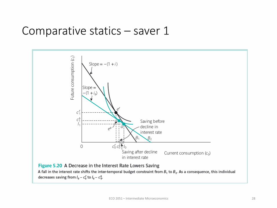
Comparative statics – saver 1


Comparative statics - saver 2


The impact of taxing interest


Applications of intertemporal decision making: human capital investment

• If education leads to higher wages later in life then studying can be regarded as an investment.

• As before, there are a stream of benefits and a stream of costs.

• By being here you have implicitly calculated that the NPV of this investment is positive(?!?).

• It is clear that a number of factors should influence this decision.• The cost of fees.• Available borrowing arrangements (students currently pay below the market

rate of interest).• Income foregone when studying.• Expected income on graduation.


A representation of the investment decision with no credit markets


Notice that here the that human capital options are entirely continuous. This is probably not the case in reality.

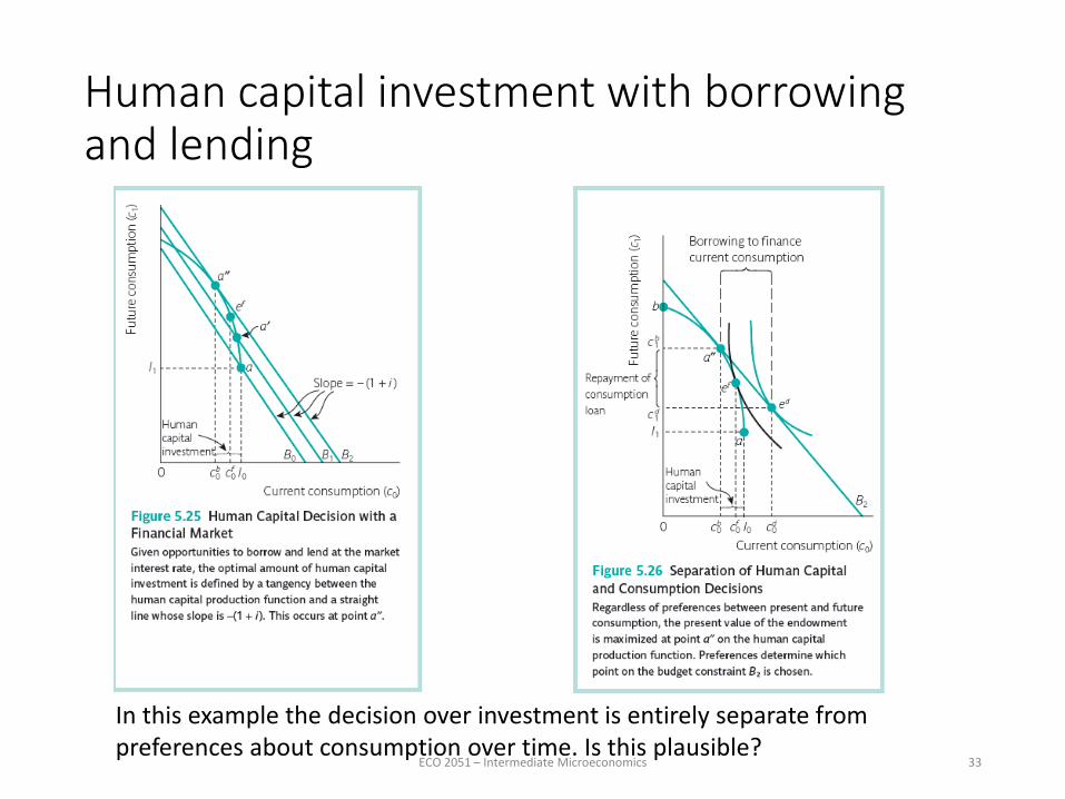
Human capital investment with borrowing and lending


In this example the decision over investment is entirely separate from preferences about consumption over time. Is this plausible?

Summary

• In a world with perfect credit markets consumers can choose between consumption today and in the future.• This is relevant for their saving and borrowing behaviour, and the approach

to investments.

• However, all these decisions will be affected by the relative price of consumption in different periods as indicated by the interest rate.

• NPV is an important concept which enables individuals to evaluate the worth of income and payments at different times.• When making decisions we should be choosing those with the highest net

present value.


lecture 5 intertemporal choice

Documents