lecture 5: linear regression with regularization csc...

Lecture 5: Linear Regression with Regularization

CSC 84020 - Machine Learning

Andrew Rosenberg

February 19, 2009

Today

Linear Regression with Regularization

Recap

Linear Regression

Given a target vector t, and data matrix X.

Goal: Identify the best parameters for a regression functiony = w0 +

∑

N

i=1 wixi

w = (XTX)−1XT t

Closed form solution for linear regression

This solution is based on

Maximum Likelihood estimation under an assumption ofGaussian Likelihood

Empirical Risk Minimization under an assumption of SquaredError

The extension of Basis Functions gives linear regression significantpower.

Revisiting overfitting

Overfitting occurs when a model captures idiosyncrasies of theinput data, rather than generalizing.

Too many parameters relative to the amount of training data

For example, an order-N polynomial can be exact fit to N + 1 datapoints.

Overfitting Example

Avoiding Overfitting

Ways of detecting/avoiding overfitting.

Use more data

Evaluate on a parameter tuning set

Regularization

Take a Bayesian approach

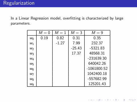
Regularization

In a Linear Regression model, overfitting is characterized by largeparameters.

M = 0 M = 1 M = 3 M = 9

w0 0.19 0.82 0.31 0.35w1 -1.27 7.99 232.37w2 -25.43 -5321.83w3 17.37 48568.31w4 -231639.30w5 640042.26w6 -1061800.52w7 1042400.18w8 -557682.99w9 125201.43

Regularization

Introduce a penalty term for the size of the weights.

Unregularized Regression

E (w) =1

2

N−1∑

n=0

{tn − y(xn,w)}2

Regularized Regression(L2-Regularization or Ridge Regularization)

E (w) =1

2

N−1∑

n=0

(tn − y(xn,w))2 +λ

2‖w‖2

Note: Large λ leads to higher complexity penalization.

Least Squares Regression with L2-Regularization

∇w(E (w)) = 0


∇w(E (w)) = 0

∇w

(

1

2

N−1∑

i=0

(y(xi ,w) − ti)2 +

λ

2‖w‖2

)

= 0

∇w

(

1

2‖t − Xw‖2 +

λ

2‖w‖2

)

= 0


∇w(E (w)) = 0

∇w

(

1

2

N−1∑

i=0

(y(xi ,w) − ti)2 +

λ

2‖w‖2

)

= 0

∇w

(

1

2‖t − Xw‖2 +

λ

2‖w‖2

)

= 0

∇w

(

1

2(t − Xw)T (t − Xw) +

λ

2wTw

)

= 0


∇w

„

1

2(t − Xw)T (t − Xw) +

λ

2w

Tw

«

= 0


∇w

„

1

2(t − Xw)T (t − Xw) +

λ

2w

Tw

«

= 0

−XTt + X

TXw + ∇w

„

λ

2w

Tw

«

= 0


∇w

„

1

2(t − Xw)T (t − Xw) +

λ

2w

Tw

«

= 0

−XTt + X

TXw + ∇w

„

λ

2w

Tw

«

= 0

−XTt + X

TXw + λw = 0


∇w

„

1

2(t − Xw)T (t − Xw) +

λ

2w

Tw

«

= 0

−XTt + X

TXw + ∇w

„

λ

2w

Tw

«

= 0

−XTt + X

TXw + λw = 0

−XTt + X

TXw + λIw = 0


∇w

„

1

2(t − Xw)T (t − Xw) +

λ

2w

Tw

«

= 0

−XTt + X

TXw + ∇w

„

λ

2w

Tw

«

= 0

−XTt + X

TXw + λw = 0

−XTt + X

TXw + λIw = 0

−XTt + (XT

X + λI)w = 0


∇w

„

1

2(t − Xw)T (t − Xw) +

λ

2w

Tw

«

= 0

−XTt + X

TXw + ∇w

„

λ

2w

Tw

«

= 0

−XTt + X

TXw + λw = 0

−XTt + X

TXw + λIw = 0

−XTt + (XT

X + λI)w = 0

(XTX + λI)w = X

Tt


∇w

„

1

2(t − Xw)T (t − Xw) +

λ

2w

Tw

«

= 0

−XTt + X

TXw + ∇w

„

λ

2w

Tw

«

= 0

−XTt + X

TXw + λw = 0

−XTt + X

TXw + λIw = 0

−XTt + (XT

X + λI)w = 0

(XTX + λI)w = X

Tt

w = (XTX + λI)−1

XTt

Regularization Results

Further Regularization

Regularization Approaches

L2-Regularization

E (w) =1

2

N−1∑

n=0

(tn − y(xn,w))2 +λ

2‖w‖2

L1-Regularization

E (w) =1

2

N−1∑

n=0

(tn − y(xn,w))2 + λ|w|1

L0-Regularization

E (w) =1

2

N−1∑

n=0

(tn − y(xn,w))2 + λ

N−1∑

n=0

δ(wn 6= 0)

The L0-norm represents the optimal subset of features needed bya Regression model.



L2-Regularization Closed form in polynomial time.

E (w) =1

2

N−1∑

n=0

(tn − y(xn,w))2 +λ

2‖w‖2

L1-Regularization

E (w) =1

2

N−1∑

n=0

(tn − y(xn,w))2 + λ|w|1

L0-Regularization

E (w) =1

2

N−1∑

n=0

(tn − y(xn,w))2 + λ

N−1∑

n=0

δ(wn 6= 0)

The L0-norm represents the optimal subset of features needed bya Regression model.How can we optimize of these functions?



L2-Regularization

E (w) =1

2

N−1∑

n=0

(tn − y(xn,w))2 +λ

2‖w‖2

L1-Regularization Can be approximated in poly-time

E (w) =1

2

N−1∑

n=0

(tn − y(xn,w))2 + λ|w|1

L0-Regularization

E (w) =1

2

N−1∑

n=0

(tn − y(xn,w))2 + λ

N−1∑

n=0

δ(wn 6= 0)




L2-Regularization

E (w) =1

2

N−1∑

n=0

(tn − y(xn,w))2 +λ

2‖w‖2

L1-Regularization

E (w) =1

2

N−1∑

n=0

(tn − y(xn,w))2 + λ|w|1

L0-Regularization NP complete optimization

E (w) =1

2

N−1∑

n=0

(tn − y(xn,w))2 + λ

N−1∑

n=0

δ(wn 6= 0)


Curse of Dimensionality

Curse of Dimensionality

Increasing the dimensionality of the feature space exponentiallyincreases the data needs.Note: The dimensionality of the feature space = The number offeatures.What is the message of this?

Models should be small relative to the amount of availabledata.

Dimensionality Reduction techniques – feature selection – canhelp.

L0-regularization is feature selection for linear models.L1- and L2-regularizations approximate feature selection and

regularize the function.

Curse of Dimensionality Example

Assume a cell requires 100 data points to generalize properly, and3-ary multinomial features.

One dimension – requires 300 data points

Two Dimensions – requires 900 data points

Three Dimensions – requires 2,700 data points

In this example, for D-dimensional model fitting, the datarequirements are 3D ∗ 10.

Argument against the Kitchen Sink approach.

Bayesians v. Frequentists

What is a Probability?



The Frequentist position

A probability is the likelihood that an event will happen.

It is approximated as the ratio of the number of times the eventhappened to the total number of events.

Assessment is very important to select a model.

Point Estimates are fine n

N



The Frequentist position

A probability is the likelihood that an event will happen.

It is approximated as the ratio of the number of times the eventhappened to the total number of events.

Assessment is very important to select a model.

Point Estimates are fine n

N

The Bayesian position

A probability is the degree of believability that the event will happen.

Bayesians require that probabilities be conditioned on data, p(y |x).

The Bayesian approach “is optimal”, given a good model, and good priorand good loss function – don’t worry about assessment as much.

Bayesians say: if you are ever making a point estimate, you’ve made amistake. The only valid probabilities are posteriors based on evidencegiven some prior.

Bayesian Linear Regression

In the previous derivation of the linear regression optimization, wemade point estimates for the weight vector, w.

Bayesians would say – “stop right there”. Use a distribution overw to estimate the parameters.

p(w|α) = N(w|0, α−1I) =( α

2π

)(M+1)/2exp

{

−α

2wTw

}

α is a hyperparameter over w, where α is the precision or inversevariance of the distribution.

So, optimize

p(w|x, t, α, β) ∝ p(t|x,w, β)p(w|α)



Again, optimizing the log likelihood yields a simpler solution.

ln p(t|x,w, β) + ln p(w|α)

p(t|x,w, β) =

N−1∏

n=0

β√2π

exp

{

−β

2(tn − y(xn,w))2

}

ln p(t|x,w, β) =N

2lnβ − N

2ln 2π − β

2

N−1∑

n=0

(tn − y(xn,w))2





ln p(t|x,w, β) =N

2lnβ − N

2ln 2π − β

2

N−1∑

n=0

(tn − y(xn,w))2

p(w|α) = N(w|0, α−1I) =( α

2π

)(M+1)/2exp

{

−α

2wTw

}

ln p(w|α) =M + 1

2lnα − M + 1

2ln 2π − α

2wTw





ln p(t|x,w, β) =N

2lnβ − N

2ln 2π − β

2

N−1∑

n=0

(tn − y(xn,w))2

ln p(w|α) =M + 1

2lnα − M + 1

2ln 2π − α

2wTw





ln p(t|x,w, β) =N

2lnβ − N

2ln 2π − β

2

N−1∑

n=0

(tn − y(xn,w))2

ln p(w|α) =M + 1

2lnα − M + 1

2ln 2π − α

2wTw

ln p(t|x,w, β) + ln p(w|α) =β

2

N−1∑

n=0

(tn − y(xn,w))2 +α

2wTw

Broader Context

Overfitting is bad.

Bayesians v. Frequentists.

Does it matter which camp you lie in?

Not particularly, but Bayesian approaches allow us some usefulinteresting and principled tools.

Bye

NextCategorization

Logistic RegressionNaive Bayes

lecture 5: linear regression with regularization csc...

Documents