lecture 5 - · pdf filerecap: terminology y i = ... this terminology in a picture dependent...

Lecture 5

In the last lecture, we covered

1. homework

2. The linear regression model (4.1)

3. Estimating the coefficients (4.2)

1

3. Estimating the coefficients (4.2)

This lecture introduces you to

1. Measures of Fit (4.3)

2. The Least Square Assumptions (4.4)

3. Sampling Distribution of the OLS estimators (4.5)

Recap: terminology

Yi = β0 + β1Xi + ui, i = 1,…, n

2

•Dependent

variable

•Regressand

•Left-hand

variable

•independent

variable

•Regressor

•Right-hand

variable

error term

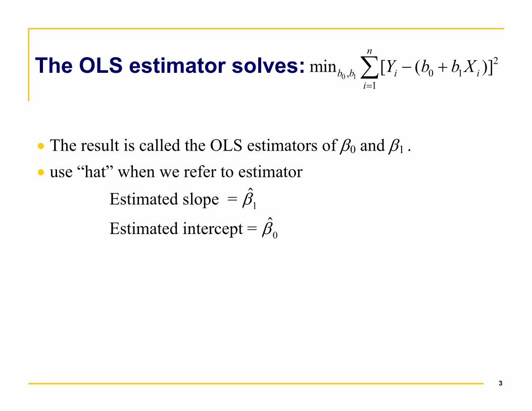
The OLS estimator solves: 0 1

2

, 0 1

1

min [ ( )]n

b b i i

i

Y b b X=

− +∑

• The result is called the OLS estimators of β0 and β1 .

• use “hat” when we refer to estimator

Estimated slope = 1β̂

3

Estimated slope = 1β

Estimated intercept = 0β̂

The OLS Linear Regression Model –

general notation

Actual value

residual

4

Yi = ˆiY + ˆ

iu , i = 1,…, n

Predicted value

where

ii XY 10ˆˆˆ ββ += i = 1,…, n

estimators

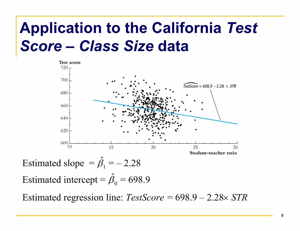
Application to the California Test

Score – Class Size data

5

Estimated slope = 1β̂ = – 2.28

Estimated intercept = 0β̂ = 698.9

Estimated regression line: �TestScore = 698.9 – 2.28× STR

Interpretation of the estimated slope and intercept

�TestScore = 698.9 – 2.28×STR

• Test score

STR

∆

∆ = –2.28

6

STR∆• what if zero students?

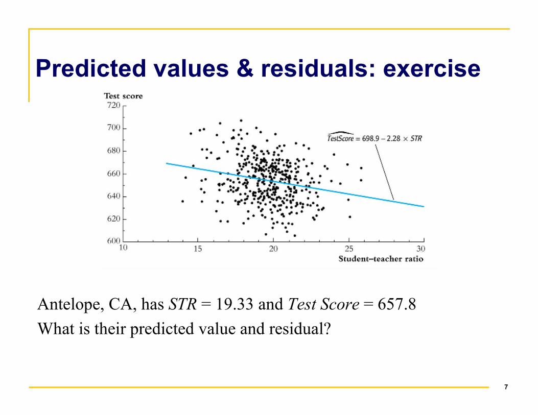
Predicted values & residuals: exercise

7

Antelope, CA, has STR = 19.33 and Test Score = 657.8

What is their predicted value and residual?

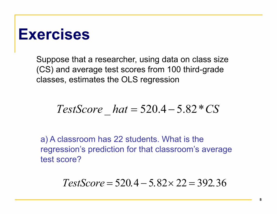
Exercises

Suppose that a researcher, using data on class size

(CS) and average test scores from 100 third-grade

classes, estimates the OLS regression

CShatTestScore *82.54.520_ −=

8


a) A classroom has 22 students. What is the

regression’s prediction for that classroom’s average

test score?

� 520 4 5 82 22 392 36TestScore = . − . × = .

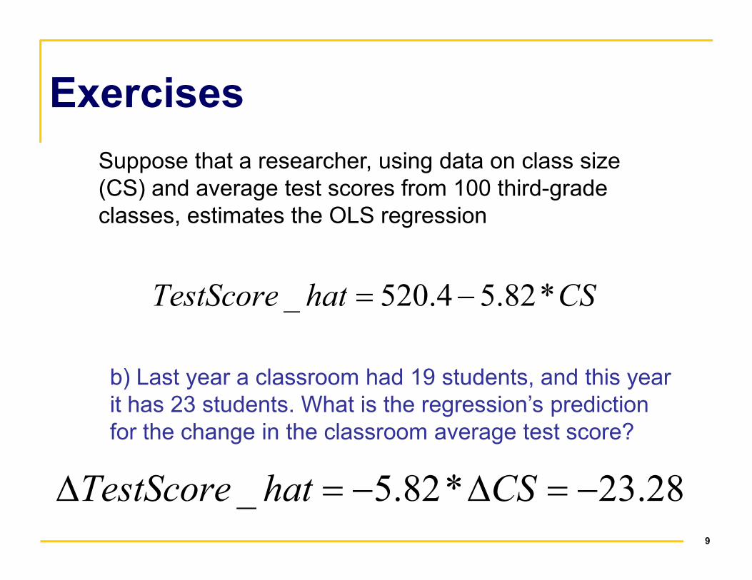
Exercises





9


b) Last year a classroom had 19 students, and this year

it has 23 students. What is the regression’s prediction

for the change in the classroom average test score?

28.23*82.5_ −=∆−=∆ CShatTestScore

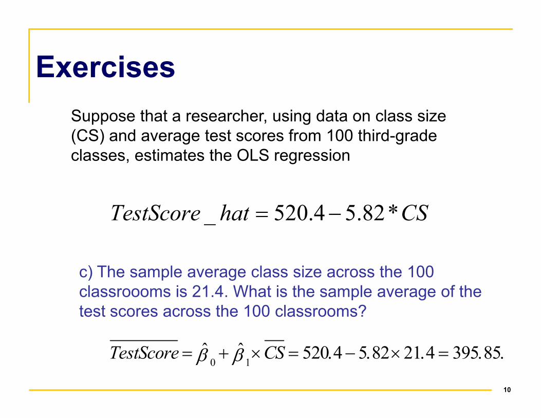
Exercises





10


c) The sample average class size across the 100

classroooms is 21.4. What is the sample average of the

test scores across the 100 classrooms?

0 1ˆ ˆ 520 4 5 82 21 4 395 85TestScore CSβ β= + × = . − . × . = . .

Measures of Fit

(Section 4.3)

how well does the regression line “fit” the data?

√ The regression R2

√ The standard error of the regression (SER)

11

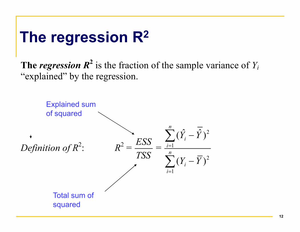
The regression R2

The regression R2 is the fraction of the sample variance of Yi

“explained” by the regression.

Explained sum

of squared

12

Definition of R2: R

2 =

ESS

TSS =

2

1

2

1

ˆ ˆ( )

( )

n

i

i

n

i

i

Y Y

Y Y

=

=

−

−

∑

∑

Total sum of

squared

of squared

This terminology in a picture

dependent

variable

ESS

TSS

2

1

2

1

ˆ ˆ( )

( )

n

i

i

n

i

i

Y Y

Y Y

=

=

−

−

∑

∑R2 = =

Y

13

independent

variable

Consider this

point

Y

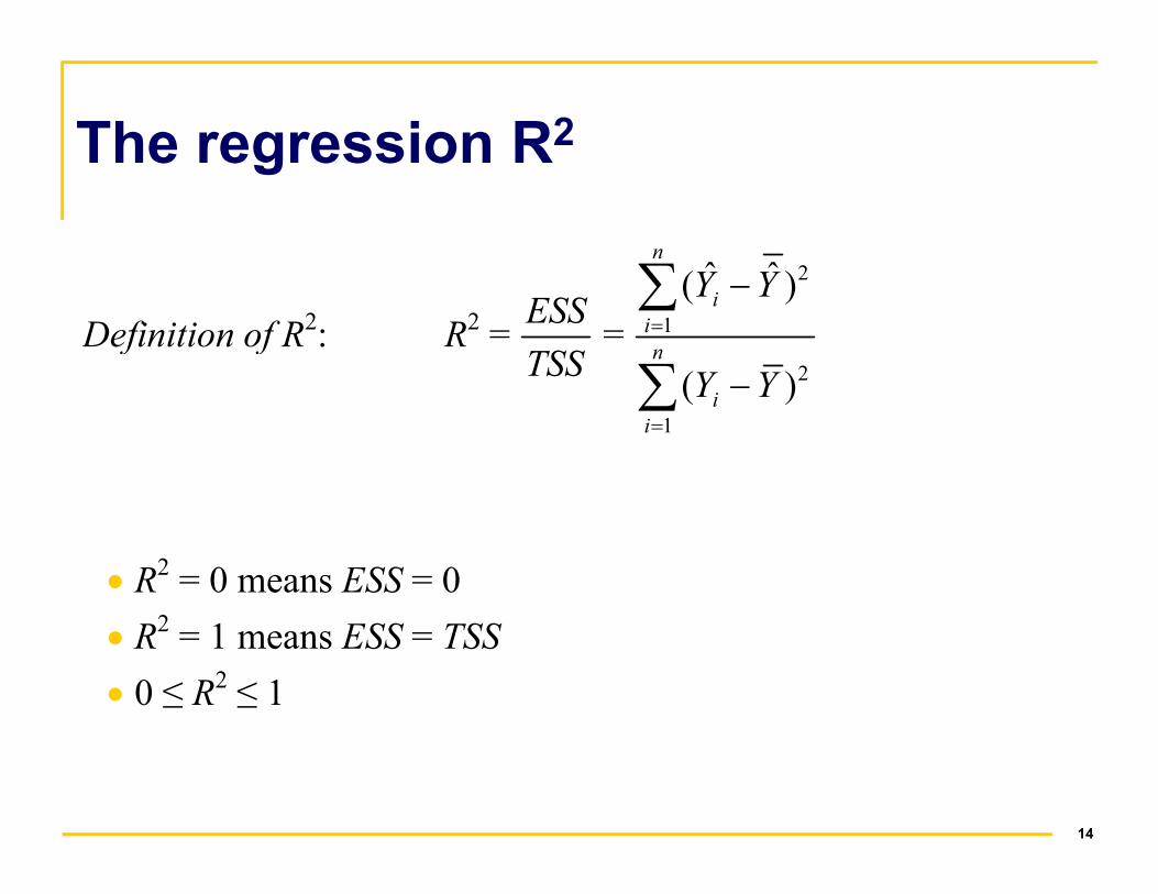
The regression R2

Definition of R2: R

2 =

ESS

TSS =

2

1

2

1

ˆ ˆ( )

( )

n

i

i

n

i

i

Y Y

Y Y

=

=

−

−

∑

∑

14

• R2 = 0 means ESS = 0

• R2 = 1 means ESS = TSS

• 0 ≤ R2 ≤ 1

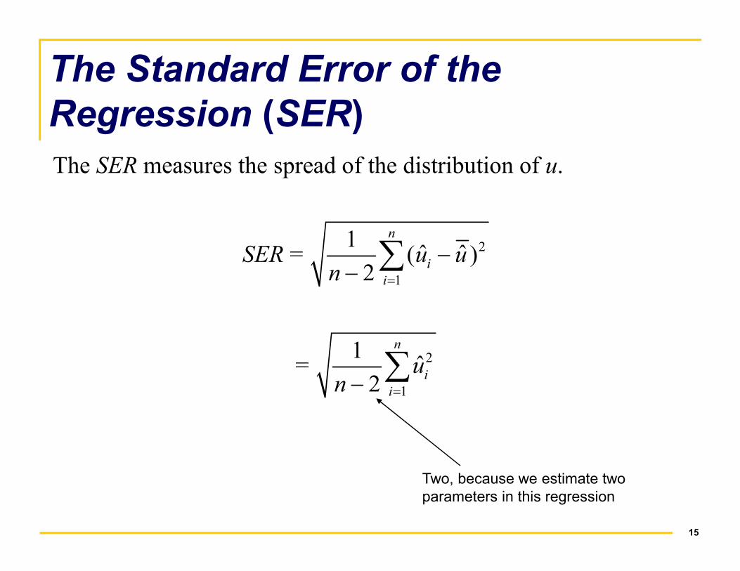
The Standard Error of the

Regression (SER)

The SER measures the spread of the distribution of u.

SER = 2

1

1ˆ ˆ( )

2

n

i

i

u un =

−− ∑

15

1i=

= 2

1

1ˆ

2

n

i

i

un =− ∑

Two, because we estimate two

parameters in this regression

The Standard Error of the

Regression (SER)

SER = 2

1

1ˆ

2

n

i

i

un =− ∑

The SER:

• has the units of u, which are the units of Y

16

• has the units of u, which are the units of Y

• measures the average “size” of the OLS residual

• The root mean squared error (RMSE) is closely related to the

SER:

RMSE = 2

1

1ˆ

n

i

i

un =∑

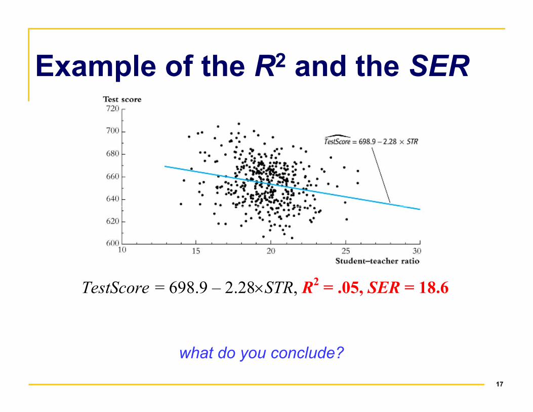
Example of the R2 and the SER

17

�TestScore = 698.9 – 2.28×STR, R2 = .05, SER = 18.6

what do you conclude?

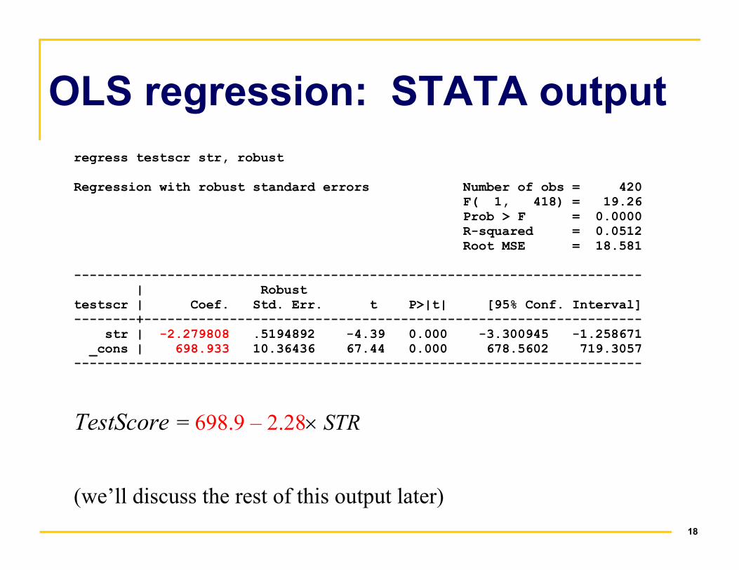
OLS regression: STATA output

regress testscr str, robust

Regression with robust standard errors Number of obs = 420 F( 1, 418) = 19.26 Prob > F = 0.0000 R-squared = 0.0512 Root MSE = 18.581 ------------------------------------------------------------------------- | Robust

18

| Robust testscr | Coef. Std. Err. t P>|t| [95% Conf. Interval] --------+---------------------------------------------------------------- str | -2.279808 .5194892 -4.39 0.000 -3.300945 -1.258671 _cons | 698.933 10.36436 67.44 0.000 678.5602 719.3057 -------------------------------------------------------------------------

�TestScore = 698.9 – 2.28× STR

(we’ll discuss the rest of this output later)

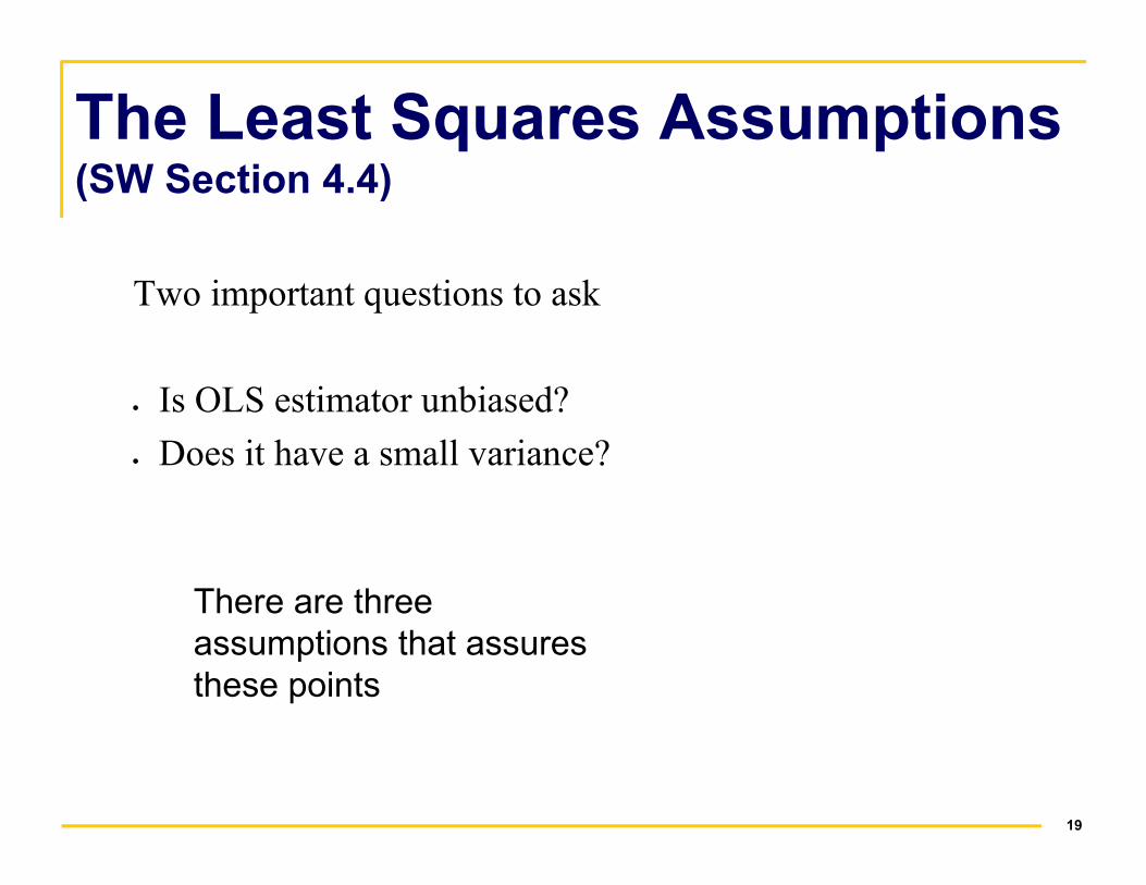
The Least Squares Assumptions (SW Section 4.4)

Two important questions to ask

• Is OLS estimator unbiased?

Does it have a small variance?

19

• Does it have a small variance?

There are three

assumptions that assures

these points

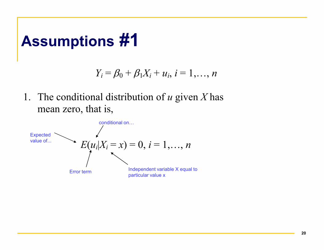
Assumptions #1

Yi = β0 + β1Xi + ui, i = 1,…, n

1. The conditional distribution of u given X has

mean zero, that is,

conditional on…

20

E(ui|Xi = x) = 0, i = 1,…, n

Expected

value of...

Error termIndependent variable X equal to

particular value x

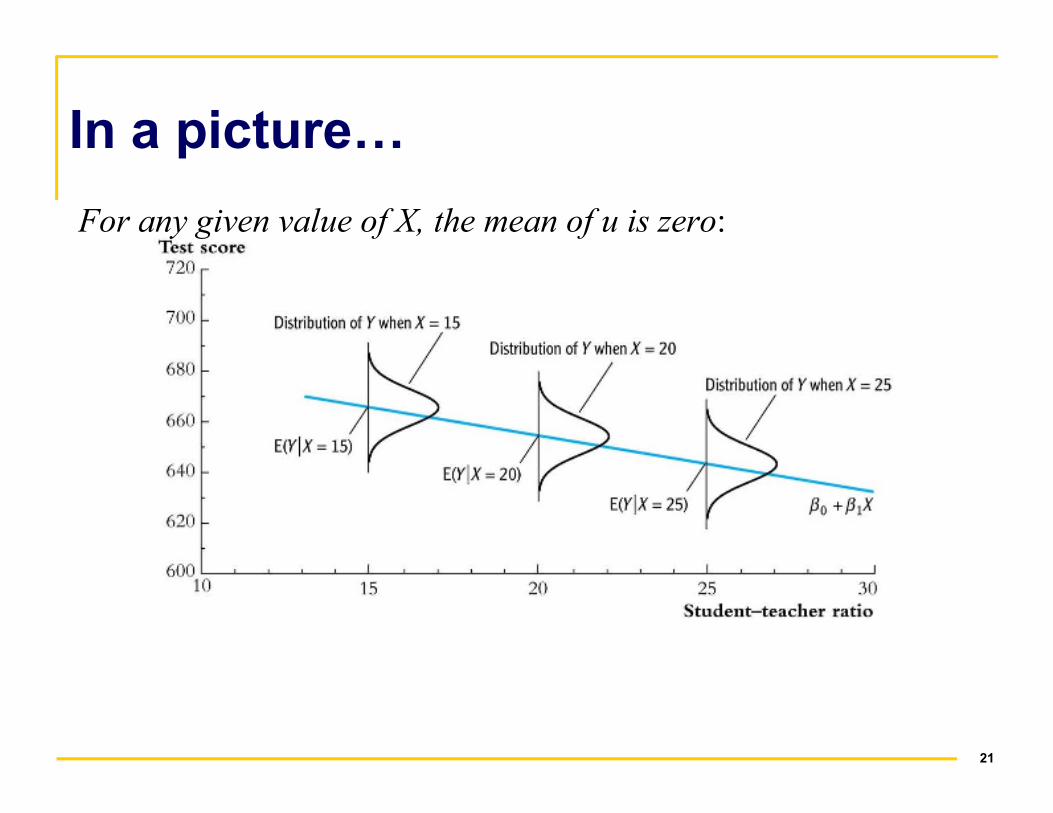
In a picture…

For any given value of X, the mean of u is zero:

21

Implication of assumption #1

corr (Xi, ui) = 0

22

in our example, Test Scorei = β0 + β1STRi + ui,

where ui = other factors

• other factor can be, for example, “English learners”

• “English learners” surely affects test performance

• if “English learners” is somehow associated with “STR”, the

above relation does not hold anymore

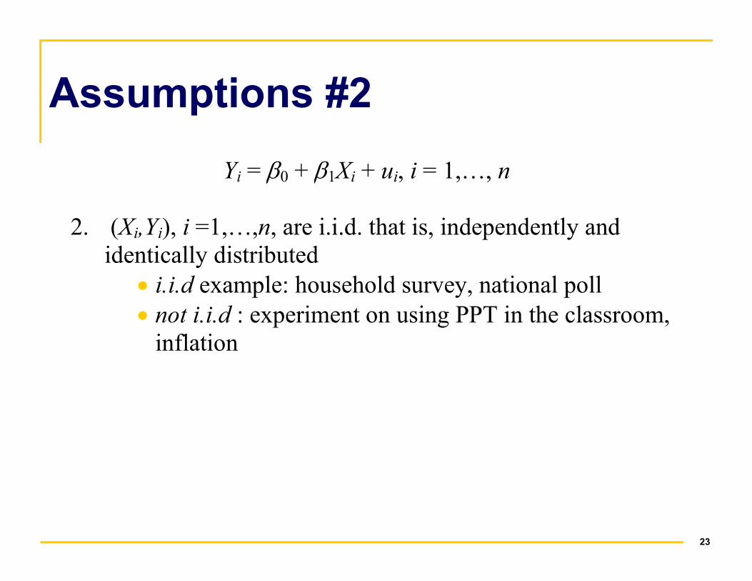
Assumptions #2

Yi = β0 + β1Xi + ui, i = 1,…, n

2. (Xi,Yi), i =1,…,n, are i.i.d. that is, independently and

identically distributed

• i.i.d example: household survey, national poll

23

• i.i.d example: household survey, national poll

• not i.i.d : experiment on using PPT in the classroom,

inflation

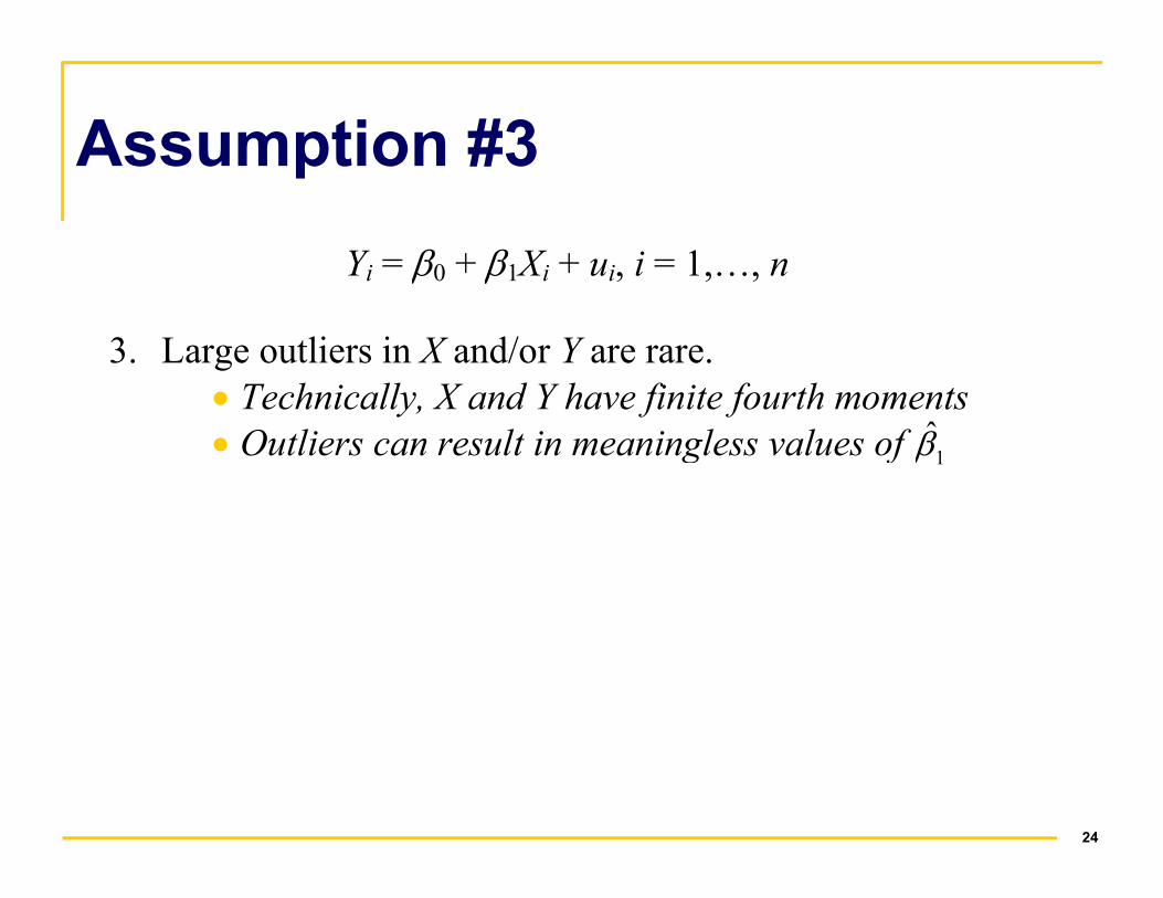
Assumption #3

Yi = β0 + β1Xi + ui, i = 1,…, n

3. Large outliers in X and/or Y are rare.

• Technically, X and Y have finite fourth moments

• Outliers can result in meaningless values of 1β̂

24

• Outliers can result in meaningless values of 1β̂

OLS can be sensitive to an outlier:

25

lecture 5 - · pdf filerecap: terminology y i = ... this terminology in a picture dependent...

Documents