lecture 6: collusion and cartels, part 2 - california...

Lecture 6: Collusion and Cartels, Part 2

EC 105. Industrial Organization. Fall 2011

Matt ShumHSS, California Institute of Technology

October 24, 2012

EC 105. Industrial Organization. Fall 2011 ( Matt Shum HSS, California Institute of Technology)Lecture 6: Collusion and Cartels, Part 2 October 24, 2012 1 / 26

Outline

Outline

1 Introduction

2 Price Wars During Booms

3 Supermarket pricing

4 Secret Price Cuts


Introduction

Does theory match reality? OPEC


Introduction

Does theory match reality? JEC


Introduction

Empirical predictions of tacit collusion

Constant production, price

Does not match empirical and anecdotal evidence from real-world cartels:defection, price-wars, etc.

Consider one such model which generates time-varying activity:Rotemberg-Saloner model

Evidence: supermarket pricing

Case study: Joint Executive Committee (railroad cartel in nineteenth-centuryUS)


Introduction

Fluctuating Demand: Rotemberg Saloner’s (1986) theoryof price wars during booms.

Demand is stochastic.

1. At each period t, it can be low (q = D1(p)) or high (q = D2(p)) withprobability 1/2 (D2(p) > D1(p) for all p). Independent across periods.

2. At each period firms learn the current state of demand before choosing theirprices simultaneously.

Look for an optimal stationary symmetric SPNE. A pair of prices {p1, p2}such that

1. Firms charge ps when the state is s,2. Prices {p1, p2} are sustainable in equilibrium3. Expected present discounted profit of each firm along the equilibrium path is

Pareto optimal

Consider infinite stream of payoffsπ0 + δπ1 + δ2π2 + · · ·+ δnπn + · · · ≡ Π(<∞). Then (1− δ)Π is implied“per-period” payoff. Convenient shorthand in what follows.


Price Wars During Booms

Price wars during booms II

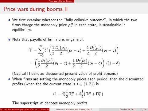
We first examine whether the “fully collusive outcome”, in which the twofirms charge the monopoly price pms in each state, is sustainable inequilibrium.

Note that payoffs of firm i are, in general:

Π̂i =∞∑t=0

δt(

1

2

D1(p1)

2(p1 − c) +

1

2

D2(p1)

2(p2 − c)

)=

(1

2

D1(p1)

2(p1 − c) +

1

2

D2(p2)

2(p2 − c)

)/(1− δ)

(Capital Π denotes discounted present value of profit stream.)

When firms are setting the monopoly prices each period, then the discountedprofits (when the the current state is s ∈ {1, 2}) is

(1− δ)1

2Πm

s + δ1

4(Πm

1 + Πm2 )

The superscript m denotes monopoly profits.



Price wars during booms III

It suffices to consider the harshest punishment of switching to competitiveprice c forever after a deviation (“Bertrand reversion”). If firm i deviates instate s obtains (1− δ)Πm

s + δ0.

Since Πm1 < Πm

2 , cheating firms will do so only in state 2; i.e., incentiveconstraint is:

(1− δ)Πm2 < (1− δ)

1

2Πm

2 + δ1

4(Πm

1 + Πm2 ) or

δ > δ ≡ 2Πm2

3Πm2 + Πm

1

∈[

1

2,

2

3

]

Temptation to undercut when demand is high. Compared to stable highdemand, face same reward and lower punishment.

When δ ∈ [1/2, δ], full collusion cannot be sustained in the high-demand state,contrary to the case of deterministic demand.



Price wars during booms IV

We now tackle the problem we set up to solve for δ ∈ [1/2, δ] (otherwise wehave either no collusion or full collusion).

Choose p1 and p2 to: max(

12

Π1(p1)2 + 1

2Π2(p2)

2

)subject to the constraints that for s = 1, 2

(1− δ)1

2Πs(ps) ≤ δ

1

4(Π1(p1) + Π2(p2))

Which can be written as:

Π1(p1) ≤ δ

2− 3δΠ2(p2) and Π2(p2) ≤ δ

2− 3δΠ1(p1)

As before, the binding constraint is that of state 2. Choosing p1 = pm1increases the objective function and relaxes the constraint for p2. Price p2 isthen chosen as high as possible:

Π2(p2) =δ

2− 3δΠm

1



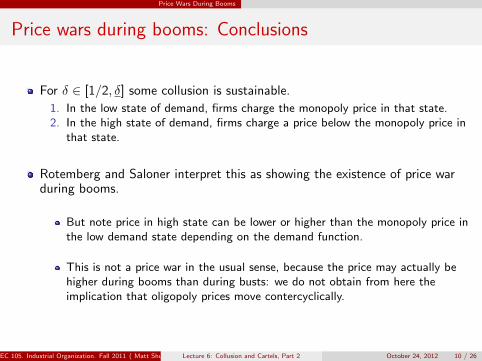
Price wars during booms: Conclusions

For δ ∈ [1/2, δ] some collusion is sustainable.

1. In the low state of demand, firms charge the monopoly price in that state.2. In the high state of demand, firms charge a price below the monopoly price in

that state.

Rotemberg and Saloner interpret this as showing the existence of price warduring booms.

But note price in high state can be lower or higher than the monopoly price inthe low demand state depending on the demand function.

This is not a price war in the usual sense, because the price may actually behigher during booms than during busts: we do not obtain from here theimplication that oligopoly prices move contercyclically.


Supermarket pricing

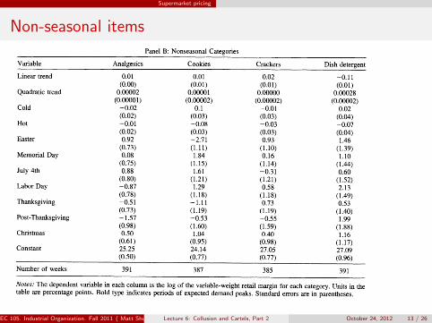
Empirical evidence: Supermarket pricing

Chevalier, Kashyap, Rossi: “Why Don’t Prices Rise During Peak Demand?”

Consider a number of grocery items.

Items have idiosyncratic peak demand periods (tuna/Lent, beer/July4)

Store also has general peak demand periods (Thanksgiving, Christmas)

Compare retail margins during peak and non-peak demand periods

Regression results


Supermarket pricing

Products with seasonal demand

VOL. 93 NO. 1 CHEVALIER ET AL.: WHY DON'T PRICES RISE DURING PEAK DEMAND?

TABLE 4-SEASONAL CHANGES IN RETAIL MARGINS

Panel A: Seasonal Categories Variable Beer Eating soup Oatmeal Cheese Cooking soup Snack crackers Tuna

Linear trend -0.21 0.04 0.04 -0.009 0.04 0.01 -0.01 (0.03) (0.01) (0.01) (0.010) (0.01) (0.01) (0.01)

Quadratic trend 0.0004 -0.00009 -0.00008 0.00006 -0.00003 0.00002 0.00006 (0.00007) (0.00002) (0.00002) (0.00002) (0.00001) (0.00002) (0.00002)

Cold -0.01 -0.07 -0.04 0.004 0.02 0.00 -0.02 (0.04) (0.03) (0.02) (0.03) (0.02) (0.03) (0.04)

Hot -0.03 -0.10 -0.02 -0.08 -0.05 -0.03 -0.07 (0.04) (0.03) (0.02) (0.03) (0.02) (0.03) (0.04)

Lent -5.03 (1.06)

Easter 0.88 0.34 0.66 -2.57 -1.49 -0.39 -1.82 (1.48) (1.07) (0.65) (1.17) (0.84) (1.20) (1.47)

Memorial Day -4.36 1.35 1.17 -0.54 0.42 1.59 -1.16 (1.44) (1.11) (0.69) (1.22) (0.87) (1.24) (1.49)

July 4th -4.08 2.18 0.27 -0.33 0.81 -1.01 1.82 (1.36) (1.18) (0.67) (1.29) (0.92) (1.31) (1.57)

Labor Day -2.61 1.42 0.19 0.27 0.05 -4.61 -1.50 (1.33) (1.15) (0.65) (1.25) (0.90) (1.28) (1.53)

Thanksgiving -1.31 1.54 0.01 -5.18 -0.68 -5.04 2.27 (1.54) (1.08) (0.66) (1.18) (0.84) (1.29) (1.36)

Post-Thanksgiving -3.12 0.87 -1.25 -4.15 0.13 -4.54 0.63 (2.00) (1.44) (0.88) (1.59) (1.13) (1.72) (1.81)

Christmas -2.66 2.34 -0.42 -3.23 0.51 -8.47 1.00 (1.25) (0.90) (0.55) (0.98) (0.70) (1.06) (1.15)

Constant 28.57 18.42 17.99 34.38 14.21 22.84 25.64 (2.88) (0.74) (1.00) (0.81) (0.58) (0.83) (0.96)

Number of weeks 219 387 304 391 387 385 339 Panel B: Nonseasonal Categories

Variable Analgesics Cookies Crackers Dish detergent Linear trend 0.01 0.01 0.02 -0.11

(0.00) (0.01) (0.01) (0.01) Quadratic trend 0.00002 0.00001 0.00000 0.00028

(0.00001) (0.00002) (0.00002) (0.00002) Cold -0.02 0.1 -0.01 0.02

(0.02) (0.03) (0.03) (0.04) Hot -0.01 -0.08 -0.03 -0.07

(0.02) (0.03) (0.03) (0.04) Easter 0.92 -2.71 0.93 1.46

(0.73) (1.11) (1.10) (1.39) Memorial Day 0.08 1.84 0.16 1.10

(0.75) (1.15) (1.14) (1.44) July 4th 0.88 1.61 -0.31 0.60

(0.80) (1.21) (1.21) (1.52) Labor Day -0.87 1.29 0.58 2.13

(0.78) (1.18) (1.18) (1.49) Thanksgiving -0.51 -1.11 0.73 0.53

(0.73) (1.19) (1.19) (1.40) Post-Thanksgiving -1.57 -0.53 -0.55 1.99

(0.98) (1.60) (1.59) (1.88) Christmas 0.50 1.04 0.40 1.16

(0.61) (0.95) (0.98) (1.17) Constant 25.25 24.14 27.05 27.09

(0.50) (0.77) (0.77) (0.96) Number of weeks 391 387 385 391

Notes: The dependent variable in each column is the log of the variable-weight retail margin for each category. Units in the table are percentage points. Bold type indicates periods of expected demand peaks. Standard errors are in parentheses.

29


Supermarket pricing

Non-seasonal items

VOL. 93 NO. 1 CHEVALIER ET AL.: WHY DON'T PRICES RISE DURING PEAK DEMAND?

TABLE 4-SEASONAL CHANGES IN RETAIL MARGINS

Panel A: Seasonal Categories Variable Beer Eating soup Oatmeal Cheese Cooking soup Snack crackers Tuna

Linear trend -0.21 0.04 0.04 -0.009 0.04 0.01 -0.01 (0.03) (0.01) (0.01) (0.010) (0.01) (0.01) (0.01)

Quadratic trend 0.0004 -0.00009 -0.00008 0.00006 -0.00003 0.00002 0.00006 (0.00007) (0.00002) (0.00002) (0.00002) (0.00001) (0.00002) (0.00002)

Cold -0.01 -0.07 -0.04 0.004 0.02 0.00 -0.02 (0.04) (0.03) (0.02) (0.03) (0.02) (0.03) (0.04)

Hot -0.03 -0.10 -0.02 -0.08 -0.05 -0.03 -0.07 (0.04) (0.03) (0.02) (0.03) (0.02) (0.03) (0.04)

Lent -5.03 (1.06)

Easter 0.88 0.34 0.66 -2.57 -1.49 -0.39 -1.82 (1.48) (1.07) (0.65) (1.17) (0.84) (1.20) (1.47)

Memorial Day -4.36 1.35 1.17 -0.54 0.42 1.59 -1.16 (1.44) (1.11) (0.69) (1.22) (0.87) (1.24) (1.49)

July 4th -4.08 2.18 0.27 -0.33 0.81 -1.01 1.82 (1.36) (1.18) (0.67) (1.29) (0.92) (1.31) (1.57)

Labor Day -2.61 1.42 0.19 0.27 0.05 -4.61 -1.50 (1.33) (1.15) (0.65) (1.25) (0.90) (1.28) (1.53)

Thanksgiving -1.31 1.54 0.01 -5.18 -0.68 -5.04 2.27 (1.54) (1.08) (0.66) (1.18) (0.84) (1.29) (1.36)

Post-Thanksgiving -3.12 0.87 -1.25 -4.15 0.13 -4.54 0.63 (2.00) (1.44) (0.88) (1.59) (1.13) (1.72) (1.81)

Christmas -2.66 2.34 -0.42 -3.23 0.51 -8.47 1.00 (1.25) (0.90) (0.55) (0.98) (0.70) (1.06) (1.15)

Constant 28.57 18.42 17.99 34.38 14.21 22.84 25.64 (2.88) (0.74) (1.00) (0.81) (0.58) (0.83) (0.96)

Number of weeks 219 387 304 391 387 385 339 Panel B: Nonseasonal Categories

Variable Analgesics Cookies Crackers Dish detergent Linear trend 0.01 0.01 0.02 -0.11

(0.00) (0.01) (0.01) (0.01) Quadratic trend 0.00002 0.00001 0.00000 0.00028

(0.00001) (0.00002) (0.00002) (0.00002) Cold -0.02 0.1 -0.01 0.02

(0.02) (0.03) (0.03) (0.04) Hot -0.01 -0.08 -0.03 -0.07

(0.02) (0.03) (0.03) (0.04) Easter 0.92 -2.71 0.93 1.46

(0.73) (1.11) (1.10) (1.39) Memorial Day 0.08 1.84 0.16 1.10

(0.75) (1.15) (1.14) (1.44) July 4th 0.88 1.61 -0.31 0.60

(0.80) (1.21) (1.21) (1.52) Labor Day -0.87 1.29 0.58 2.13

(0.78) (1.18) (1.18) (1.49) Thanksgiving -0.51 -1.11 0.73 0.53

(0.73) (1.19) (1.19) (1.40) Post-Thanksgiving -1.57 -0.53 -0.55 1.99

(0.98) (1.60) (1.59) (1.88) Christmas 0.50 1.04 0.40 1.16

(0.61) (0.95) (0.98) (1.17) Constant 25.25 24.14 27.05 27.09

(0.50) (0.77) (0.77) (0.96) Number of weeks 391 387 385 391

Notes: The dependent variable in each column is the log of the variable-weight retail margin for each category. Units in the table are percentage points. Bold type indicates periods of expected demand peaks. Standard errors are in parentheses.

29


Secret Price Cuts

Secret Price Cuts

Up to now, firm’s past choice is perfectly observed by its rival. However,(effective) prices may not be observable (discounts, quality, etc).

Must rely on observation of its own realized market share or demand todetect any price undercutting by the rival. But a low market share may bedue to the aggressive behavior of one’s rival or to a slack in demand.

Remark: Under uncertainty, mistakes are unavoidable and maximalpunishments (eternal reversion to Bertrand behavior) need not be optimal.


Secret Price Cuts

Secret Price Cuts

Framework of our basic repeated game with:

In each period, there are two possible realizations of demand (states ofnature), i.i.d..

With probability α, there is no demand for the product sold by the duopolists(the “low-demand” state).With probability 1− α, there is a positive demand D(p) (the “high-demand”state).

A firm that does not sell at some date is unable to observe whether theabsence of demand is due to the realization of the low-demand state or to itsrival’s lower price.

Remark: all or nothing demand function is an extreme simplification, but itallows us to study the problem with a nontrivial inference problem in the basicsetup; a more general approach would require us to introduce differentiatedproducts


Secret Price Cuts

Secret Price Cuts

Look for an equilibrium with the following strategies:

There is a collusive phase and a punishment phase. The game begins in thecollusive phase. Both firms charge pm until one firm makes a zero profit. (notethis is common knowledge).

The occurrence of a zero profit triggers a punishment phase. Here both firmscharge c for exactly T periods, where T can a priori be finite or infinite.

At the end (if any) of the punishment phase, the firms revert to the collusivephase.

We want to look for a length of the punishment phase such that the expectedpresent value of profits for each firm is maximal subject to the constraint thatthe associated strategies form a SPNE.


Secret Price Cuts

Secret Price Cuts

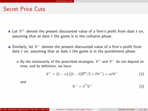
Let V+ denote the present discounted value of a firm’s profit from date t on,assuming that at date t the game is in the collusive phase.

Similarly, let V− denote the present discounted value of a firm’s profit fromdate t on, assuming that at date t the game is in the punishment phase.

By the stationarity of the prescribed strategies, V+ and V− do not depend ontime, and by definition, we have:

V+ = (1− α)((1− δ)Πm/2 + δV+) + αδV− (1)

andV− = δTV+ (2)


Secret Price Cuts

Secret Price Cuts

Since strategies need to be a SPNE, we need to include incentivecompatibility constraints ruling out profitable deviations in both phases.

Easy to see that there are no profitable one shot deviations in the punishmentphase. Thus, it suffices to consider incentives in the collusive phase. This is:

V+ ≥ (1− α)((1− δ)Πm + δV−) + α(δV−) (3)

(3) expresses the trade-off for each firm. If a firm undercuts, it getsΠm > Πm/2. However, undercutting automatically triggers the punishmentphase, which yields valuation V− instead of V+.

To deter undercutting, V− must be sufficiently lower than V+. This meansthat the punishment must last long enough.

But because punishments are costly and occur with positive probability, Tshould be chosen as small as possible given that 3 is satisfied.


Secret Price Cuts

Secret Price Cuts

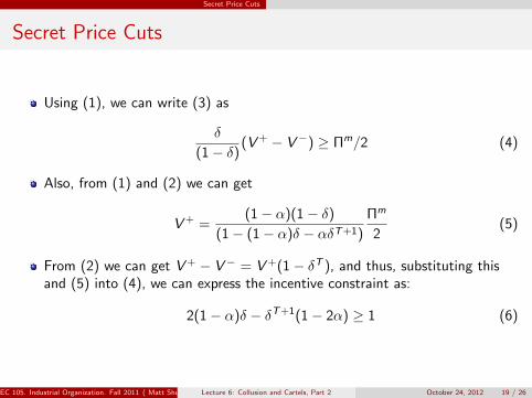
Using (1), we can write (3) as

δ

(1− δ)(V+ − V−) ≥ Πm/2 (4)

Also, from (1) and (2) we can get

V+ =(1− α)(1− δ)

(1− (1− α)δ − αδT+1)

Πm

2(5)

From (2) we can get V+ − V− = V+(1− δT ), and thus, substituting thisand (5) into (4), we can express the incentive constraint as:

2(1− α)δ − δT+1(1− 2α) ≥ 1 (6)


Secret Price Cuts

Secret Price Cuts

Note that now we can express the problem as that of maximizing V+ subjectto (6). And furthermore, since V+ is decreasing in T , we want to find thelowest T such that (6) holds.

Note that the constraint is not satisfied with T = 0, and that therefore, sincethe LHS of (6) decreases with T if α ≥ 1/2, that in this case there is nosolution (no strategy profile of this sort is a SPNE). Thus we need α < 1/2.

Assuming in fact that (1− α)δ ≥ 1/2, so that the constraint is satisfied forT →∞, there exists a (finite) optimal length of punishment T ∗ In fact,

T ∗ = int+

Ln(

2(1−α)δ−11−2α

)Ln(δ)

− 1


Secret Price Cuts

Secret Price Cuts

This model predicts periodic price wars, contrary to the perfect observationmodels.

Price wars are involuntary, in that they are triggered not by a price cut but byan unobservable slump in demand.

Note also that price wars are triggered by a recession, contrary to theRotemberg-Saloner model.


Secret Price Cuts

Secret Price Cuts

Under imperfect information, the fully collusive outcome cannot be sustained.

It could be sustained only if the firms kept on colluding (charging themonopoly price) even when making small profits, because even under collusionsmall profits can occur as a result of low demand.

However, a firm that is confident that its rival will continue cooperating evenif its profit is low has every incentive to (secretely) undercut - priceundercutting yields a short-term gain and creates no long-run loss.

Thus, full collusion is inconsistent with the deterrence of price cuts.


Secret Price Cuts

Secret Price Cuts

Oligopolists are likely to recognize the threat to collusion posed by secrecy,and take steps to eliminate it.

Industry trade associations

1. collect detailed information on the transactions executed by the members.

2. allows it members to cross-check price quotations.

3. imposes standarization agreements to discourage price-cutting when productshave multiple attributes.

4. Case study: Joint Executive Committee. Railroad cartel in the late 19th centuryUS.

Resale-price maintenance on their retailers, or “most favored nation ” clause.

1. Simplify observation and detection


Secret Price Cuts

Porter (1983): Case study of JEC

Fit data to game theoretic model where behavioral regime – “cooperative”vs. “non-cooperative” – varies over time.

Reminder: “non-cooperative” phase in repeated games models not due tocheating!

Measure market power in both regimes.

Data: Table 1

Price (GR) and quantity (grain shipments TGR)St are supply-shifters (dummies DM1, DM2, DM3, DM4 for entry byadditional rail companies)LAKESt : dummy when Great Lakes was open to traffic. Demand-shifter.


Secret Price Cuts

Porter (1983): Model

N firms (railroads), each producing a homogeneous product (grainshipments). Firm i chooses qit in period t.

Market demand: logQt = α0 + α1 log pt + α2LAKESt + U1t , whereQt =

∑i qit .

Firm i ’s cost fxn: Ci (qit) = aiqδit + Fi

Firm i ’s pricing equation: pt(1 + θitα1

) = MCi (qit), where:θit = 0: Bertrand pricingθit = 1: Monopoly pricingθit = sit : Cournot outcome

After some manipulation, aggregate supply relation is:

log pt = logD − (δ − 1) logQt − log(1 + θt/α1)

with empirical version

log pt = β0 + β1 logQt + β2St + β3It + U2t


Secret Price Cuts

Porter (1983): Results, Table 3

Estimate in two ways (results quite similar):1 Two-stage least squares2 Maximum likelihood

GR: price elasticity < 1 in abs. value. Not consistent with optimal monopolypricing.

LAKESt reduces demand;

DM variables lowered market price

Estimate of β3 is 0.382/0.545: prices higher when firms are in “cooperative”regime.

If we assume that θ = 0 in non-cooperative periods, then this implies θ=0.336in cooperative periods. Low? (Recall θ = 1 under cartel maximization)

Table 4:

prices higher and quantity lower in “noncooperative” (PN = 1) periods.Cartel earns $11,000 more in weeks when they are cooperating


lecture 6: collusion and cartels, part 2 - california...

Documents