lecture 6: finite element method i
TRANSCRIPT

Lecture 6: Finite Element Method I
Jose A. Gonzalez
Departamento de Ingenierıa de la Construccion y Proyectos de IngenierıaEscuela Tecnica Superior de Ingenierıa
Universidad de Sevilla
An ECCOMAS Advanced Course on Computational Structural DynamicsPrague, June 2018
Jose A. Gonzalez Finite Element Method I Prague 2018 1 / 38

Outline
1 Introduction
2 Principle of virtual work
3 Finite Element Formulation
4 Assembly of global matrices
5 Convergence properties
6 Example
Jose A. Gonzalez Finite Element Method I Prague 2018 2 / 38

Outline
1 Introduction
2 Principle of virtual work
3 Finite Element Formulation
4 Assembly of global matrices
5 Convergence properties
6 Example
Jose A. Gonzalez Finite Element Method I Prague 2018 3 / 38

Introduction
Non-exhaustive classification of FEM applications:
Finite Element Method
CoupledPhysics
OtherPhysics
...Electro-Magnetics
HeatTransfer
FluidMechanics
FluidFlow
Acoustics
SolidMechanics
StaticsDynamics
LinearNonlinear
In Linear problems we assume small displacements (geometry), linear materialconstitutive relation and constant/linear boundary conditions.
In Statics inertial forces are ignored or neglected.
In Dynamics the time dependence is explicitly considered because the calculation ofinertial (and/or damping) forces requires derivatives respect to actual time to betaken.
In this lecture, we will restrict ourselves to the pure displacement formulation oflinear elastodynamics.
Jose A. Gonzalez Finite Element Method I Prague 2018 4 / 38

Linear Elasticity
Governing equations of linear elasticity in tensor form Link
Equation of motion, which is an expression of Newton’s second law:
ρu−∇ · σ = b
where u is the displacement vector, b is the body force per unit volume, ρ is themass density and σ is the Cauchy stress tensor.Strain-displacement relation:
ε = 12[∇u + ∇Tu]
where ε is the infinitesimal strain tensor.Constitutive equation:
σ = D : ε
where D is the fourth-order constitutive tensor.For elastic materials, Hooke’s law.Boundary conditions:
u = u (Dirichlet)
t = σ · n = t (Neumann)
where n is the unit normal to the boundaryJose A. Gonzalez Finite Element Method I Prague 2018 5 / 38

Outline
1 Introduction
2 Principle of virtual work
3 Finite Element Formulation
4 Assembly of global matrices
5 Convergence properties
6 Example
Jose A. Gonzalez Finite Element Method I Prague 2018 6 / 38

Strong Form of Elastodynamics
Initial Value Problem (IVP)
ρu−∇ · σ = b in Ωu = u on Γu
t = t on Γtu(x, 0) = u0 in Ωu(x, 0) = u0 in Ω
where u(x, t) are the displacements of the solid for time t at coordinate x = (x , y),t = σ · n the boundary tractions and b(x) are the body loads.
x
y
u
n
t
t
Jose A. Gonzalez Finite Element Method I Prague 2018 7 / 38

Principle of virtual work
Weak statement of the dynamic equilibrium of the body
δW (u; δu) =
∫Ω
δu · (ρu−∇ · σ − b) dΩ = 0
where δu(x) is an arbitrary virtual displacement or weight function.
2nd order space derivatives of u can be reduced to 1st order using the relation
∇ · (σ · δu) = δu · (∇ · σ) + σ : ∇δu
integrating in Ω and after applying the divergence theorem (Gauss) we obtain:∮Γ
δu · (σ · n) dΓ =
∫Ω
δu · (∇ · σ) dΩ +
∫Ω
σ : ∇δu dΩ
Finally, substituting this into the weak form:
δW (u; δu) =
∫Ω
[δu · ρu− δu · (∇ · σ)− δu · b] dΩ = 0
we obtain...
Jose A. Gonzalez Finite Element Method I Prague 2018 8 / 38

Obtaining the weak form
Principle of Virtual Work (weak form of the IVP):
δW (u; δu) =
∫Ω
σ : δε dΩ−∫
Ω
δu · (b− ρu) dΩ−∮
Γ
δu · t dΓ = 0
We have reduced the continuity requirement of u from C 2(Ω) to C 1(Ω).
In particular, we can apply this principle to an element with domain Ωe andboundary Γe :
δW e =
∫Ωe
σ : δε dΩ−∫
Ωe
δu · (b− ρu) dΩ−∮
Γeδu · t dΓ = 0
where n is now the unit outward normal to Γe .
Shape functions must be C 0(Γe) continuous between interconnected elements, andC 1(Ωe) piecewise differentiable inside each element.
Jose A. Gonzalez Finite Element Method I Prague 2018 9 / 38

Outline
1 Introduction
2 Principle of virtual work
3 Finite Element Formulation
4 Assembly of global matrices
5 Convergence properties
6 Example
Jose A. Gonzalez Finite Element Method I Prague 2018 10 / 38

Steps of the Finite Element Analysis
Step 1 The continuum Ω is divided into ne elements Ωe of simple geometrydenominated Finite Elements.
Ω =
ne⋃e=1
Ωe
Step 2 The elements are assumed to be interconnected at nn nodal points situated ontheir boundaries and occasionally in their interior. The displacements of theseNodes will be the basic unknowns (DOFs) of the problem.
Step 3 A set of Shape Functions at least C 1(Ω)-continuous inside the element ischosen to define uniquely the state of displacement within each finite elementand on its boundaries in terms of its nodal displacements.
Step 4 The displacement functions are derived to compute the element strains withinan element in terms of the nodal displacements.
Step 5 Use of the material constitutive relation to compute the element stresses.
Step 6 Selection of the discrete weighting functions (virtual displacementsapproximation).
Step 7 Substitute all these discrete approximations in the PTV.
Jose A. Gonzalez Finite Element Method I Prague 2018 11 / 38

Discretization
Particular case of plane-stress (2D):
x
y
u
n
t
t
Jose A. Gonzalez Finite Element Method I Prague 2018 12 / 38

Discretization
Particular case of plane-stress (2D):
x
y
u
n
t
t
Jose A. Gonzalez Finite Element Method I Prague 2018 12 / 38

Discretization
Particular case of plane-stress (2D):
i
j
k
x
y
e
u
n
t
t
Jose A. Gonzalez Finite Element Method I Prague 2018 12 / 38

Displacements approximation
Particular case of plane-stress (2D):
Definition of C 1(Ωe) shape functions (approximation functions):
u(x , y) =
u(x , y)v(x , y)
≈
nn∑j=1
Nej (x , y)de
j
For a linear triangular element:
METU – Dept. of Mechanical Engineering – ME 413 Int. to Finite Element Analysis – Lecture Notes of Dr. Sert 5-7
2D Formulation (cont’d)
• Approximate solution over an element is
𝑢𝑒 = 𝑢𝑗𝑒 𝑆𝑗𝑒(𝑥, 𝑦)𝑁𝐸𝑁
𝑗=1
• For linear triangular and quadratic elements 𝑁𝐸𝑁 is 3 and 4, respectively.
3-node triangular element 𝑁𝐸𝑁 = 3
4-node quadrilateral element 𝑁𝐸𝑁 =4
3-node triangular element Ωe
nn = 3
i
j
k
1
y
N (x,y)k
x
Approximate solution over an element is:
u(x) =
nn∑j=1
Nej (x)de
j =[Ni Nj Nk
]di
dj
dk
e
= Nde
where Nα = Nα I2 (α = i , j , k).
Jose A. Gonzalez Finite Element Method I Prague 2018 13 / 38

Displacements approximation
For the 3-node triangular element:
Shape functions:
i
j
k
Ae
(xi, yi)(xj , yj)
(xk, yk) Ni (x , y) = 1
2Ae (αi + βix + γiy)
Nj(x , y) = 12Ae (αj + βjx + γjy)
Nk(x , y) = 12Ae (αk + βkx + γky)
Partition of unity and Kronecker δ property:
Ni (xi , yi ) = 1 Ni (xj , yj) = 0 Ni (xk , yk) = 0
Nj(xi , yi ) = 0 Nj(xj , yj) = 1 Nj(xk , yk) = 0
Nk(xi , yi ) = 0 Nk(xj , yj) = 0 Nk(xk , yk) = 1
solving for α, β and γ:
αi = xjyk − yjxk βi = yj − yk γi = xk − xj
αj = xiyk − yixk βj = yk − yi γj = xi − xk
αk = xiyj − yixj βk = yi − yj γk = xj − xi
The element area is calculated as:
2Ae = xiβi + xjβj + xkβkJose A. Gonzalez Finite Element Method I Prague 2018 14 / 38

Strains
Once you know the displacements, the strains are computed by derivation:
Strains-displacement relation
ε = Su = SNde = Bde
where S is a linear differential operator and B is the strains approximation matrix.Particular case of plane-stress (2D):
Strain-displacement relation:
ε =
εxεyγxy
=
∂u∂x∂v∂y
∂u∂y
+ ∂v∂x
=
∂∂x
00 ∂
∂y∂∂y
∂∂x
︸ ︷︷ ︸
S
uv
︸ ︷︷ ︸
u
and because in the element u = Nde , the strain approximation matrix B = SN canbe determined:
B =
∂∂x
00 ∂
∂y∂∂y
∂∂x
[Ni 0 Nj 0 Nk 00 Ni 0 Nj 0 Nk
]=
∂Ni∂x
0∂Nj
∂x0 ∂Nk
∂x0
0 ∂Ni∂y
0∂Nj
∂y0 ∂Nk
∂y∂Ni∂y
∂Ni∂x
∂Nj
∂y
∂Nj
∂x∂Nk∂y
∂Nk∂x
Jose A. Gonzalez Finite Element Method I Prague 2018 15 / 38
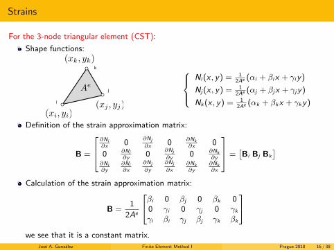
Strains
For the 3-node triangular element (CST):
Shape functions:
i
j
k
Ae
(xi, yi)(xj , yj)
(xk, yk) Ni (x , y) = 1
2Ae (αi + βix + γiy)
Nj(x , y) = 12Ae (αj + βjx + γjy)
Nk(x , y) = 12Ae (αk + βkx + γky)
Definition of the strain approximation matrix:
B =
∂Ni∂x
0∂Nj
∂x0 ∂Nk
∂x0
0 ∂Ni∂y
0∂Nj
∂y0 ∂Nk
∂y∂Ni∂y
∂Ni∂x
∂Nj
∂y
∂Nj
∂x∂Nk∂y
∂Nk∂x
=[Bi Bj Bk
]Calculation of the strain approximation matrix:
B =1
2Ae
βi 0 βj 0 βk 00 γi 0 γj 0 γkγi βi γj βj γk βk
we see that it is a constant matrix.
Jose A. Gonzalez Finite Element Method I Prague 2018 16 / 38

Stresses
In general, the material can be subjected to initial strains ε0 and initial residual stressesσ0 wich are a-priori known.
Constitutive relation
σ = D(ε− ε0) + σ0
where D is an elasticity matrix containing the appropriate material properties.In the particular case of plane-stress (2D):
Introducing an isotropic stress-strain linear relationship:
σ =
σx
σy
τxy
ε =
εxεyγxy
εx − (εx)0 =
1
Eσx −
ν
Eσy
εy − (εy )0 =1
Eσy −
ν
Eσx
γxy − (γxy )0 =2(1 + ν)
Eτxy
and solving for the stresses:
D =E
1− ν2
1 ν 0ν 1 00 0 1
2(1− ν)
Jose A. Gonzalez Finite Element Method I Prague 2018 17 / 38

2D Displacement Formulation
To derive the Finite Element Equations we proceed as follows:I Substitute approximation of displacements
u(x, t) =
nn∑i=1
Ni (x)di (t)
and accelerations
u(x, t) =
nn∑i=1
Ni (x)di (t)
into the weak form.I Use the same functions as test functions (this is known as Galerkin approximation)
δu(x, t) =
nn∑i=1
Ni (x)δdi , δε(x, t) =
nn∑i=1
Bi (x)δdi
Arrange to get:
δdTne∑e=1
∫
Ωe
ρNTN dΩ︸ ︷︷ ︸Me
d +
∫Ωe
BTDB dΩ︸ ︷︷ ︸Ke
d
= δdTne∑e=1
∫
Ωe
NTb dΩ︸ ︷︷ ︸feb
+
∮Γe
NTt dΓ︸ ︷︷ ︸fet
Jose A. Gonzalez Finite Element Method I Prague 2018 18 / 38

2D Displacement Formulation
The FEM equations for one element e can be written:
Me de + Ke de = feb + fet = fe
Me =
∫Ωe
ρNeTNe dΩ
Ke =
∫Ωe
BeTDBe dΩ
fet =
∮Γe
NeTt dΓ
feb =
∫Ωe
NeTb dΩ
Normally, to evaluate these 2D integrals:I Triangular and quadrilateral master elements will be introduced.I Shape functions will be written in master element coordinates.I 2D Jacobian transformation will be used.I Gauss Quadrature numerical integration will be used.
The assembly of all the element contributions, provides the global FEM equations:
Semidiscrete FEM equations
Md + Kd = f
where f includes the body forces and the external tractions.
Jose A. Gonzalez Finite Element Method I Prague 2018 19 / 38

2D Displacement Formulation
Matlab function: elementMatrices.m
function [Ke,Me] = elementMatrices(E,NU,RHO,t,xi,yi,xj,yj,xk,yk,p)% Use p = 1 for plane-stress and p = 2 for plane-strain% AreaA = (xi*(yj-yk) + xj*(yk-yi) + xk*(yi-yj))/2;% Deformation matrixbetai = yj-yk; betaj = yk-yi; betak = yi-yj;gammai = xk-xj; gammaj = xi-xk; gammak = xj-xi;B = [betai 0 betaj 0 betak 0;0 gammai 0 gammaj 0 gammak;gammai betai gammaj betaj gammak betak]/(2*A);
% Constitutive matrixif p == 1D = (E/(1-NU*NU))*[1 NU 0 ; NU 1 0 ; 0 0 (1-NU)/2];
elseif p == 2D = (E/(1+NU)/(1-2*NU))*[1-NU NU 0 ; NU 1-NU 0 ; 0 0 (1-2*NU)/2];
end% Stiffness matrixKe = t*A*B'*D*B;% Mass matrixMe = (RHO*t*A/12)*[2 0 1 0 1 0;0 2 0 1 0 1;1 0 2 0 1 0;0 1 0 2 0 1;1 0 1 0 2 0;0 1 0 1 0 2];end
Jose A. Gonzalez Finite Element Method I Prague 2018 20 / 38
Outline
1 Introduction
2 Principle of virtual work
3 Finite Element Formulation
4 Assembly of global matrices
5 Convergence properties
6 Example
Jose A. Gonzalez Finite Element Method I Prague 2018 21 / 38

Assembly of global matrices
Let us assume a 2D mesh with 1DOF per node:
ME 582 Finite Element Analysis in Thermofluids Dr. Cüneyt Sert
3-7
Figure 3.4 Element and global and local node numbering for a sample 2D mesh
To perform the assembly we need to write the local-to-global node mapping matrix. To do this first we need to select a global node numbering and then a local node numbering for each element, which can be as the ones shown in Figure 3.4. With the selected global and local node numberings local-to-global node mapping matrix can be written as follows
[
]
where the entry of the last row does not exist since the third element has only three nodes. Using the assembly rule and this matrix, the following global stiffness matrix
[
4
3
4 3
4 3
4 3
4 4
44
3 43
3 43 3
3
3 3
4 4
34
3 33 44
3
4 43
4 43 3
3 34
3 3
34
4 33
4 34
4 3 4
3 443 43
3
3 3 3
3 3 4 3
4 343 33
3 334 ]
and the following global force vector and boundary integral vector can be obtained
4 3
3 4
3 4
3
43 4
33 3
4
4
3
3 4
3
4
3
43
4
33 3
4
x 1 2
” 3
4 5 6
7 8
y e=1 e=2
e=3 e=4
x 1
y e=1 e=2
e=3 e=4
2
4 3
1 2
4 3 1 2
4 3
1 2
3
The global DOF mapping matrix m reserves a position mi,j in the global system forthe j-DOF of the i-element:
m =
1 2 5 42 3 6 54 5 8 75 6 8 x
Jose A. Gonzalez Finite Element Method I Prague 2018 22 / 38

Assembly of global matrices
Applying the assembly process to all the element stiffness matrices:
for e = 1 . . . ne
indexs = m(e, :)
M(indexs, indexs) = M(indexs, indexs) + Me
K(indexs, indexs) = K(indexs, indexs) + Ke
end for
we obtain the global mass and stiffness matrix:
ME 582 Finite Element Analysis in Thermofluids Dr. Cüneyt Sert
3-7
Figure 3.4 Element and global and local node numbering for a sample 2D mesh
To perform the assembly we need to write the local-to-global node mapping matrix. To do this first we need to select a global node numbering and then a local node numbering for each element, which can be as the ones shown in Figure 3.4. With the selected global and local node numberings local-to-global node mapping matrix can be written as follows
[
]
where the entry of the last row does not exist since the third element has only three nodes. Using the assembly rule and this matrix, the following global stiffness matrix
[
4
3
4 3
4 3
4 3
4 4
44
3 43
3 43 3
3
3 3
4 4
34
3 33 44
3
4 43
4 43 3
3 34
3 3
34
4 33
4 34
4 3 4
3 443 43
3
3 3 3
3 3 4 3
4 343 33
3 334 ]
and the following global force vector and boundary integral vector can be obtained
4 3
3 4
3 4
3
43 4
33 3
4
4
3
3 4
3
4
3
43
4
33 3
4
x 1 2
” 3
4 5 6
7 8
y e=1 e=2
e=3 e=4
x 1
y e=1 e=2
e=3 e=4
2
4 3
1 2
4 3 1 2
4 3
1 2
3
Jose A. Gonzalez Finite Element Method I Prague 2018 23 / 38

Assembly of global matrices
Matlab function: globalMatrices.m
function [K,M] = globalMatrices(mesh,material)% dimensionsnnodes=size(mesh.Nodes,2);nelements=size(mesh.Elements,2);ndofs=2*nnodes;K=zeros(ndofs);M=zeros(ndofs);for e=1:nelements
% element connectivityi = mesh.Elements(1,e);j = mesh.Elements(2,e);k = mesh.Elements(3,e);% nodal coordintesxi = mesh.Nodes(1,i); yi = mesh.Nodes(2,i);xj = mesh.Nodes(1,j); yj = mesh.Nodes(2,j);xk = mesh.Nodes(1,k); yk = mesh.Nodes(2,k);% element matrices[ke,me] = elementMatrices(material.E,material.nu,material.rho,material.t,xi,yi,xj,yj,xk,yk,1);% global dof positionsin=[2*i-1 2*i 2*j-1 2*j 2*k-1 2*k];% assemblingK(in,in)=K(in,in)+ke; M(in,in)=M(in,in)+me;
end
Jose A. Gonzalez Finite Element Method I Prague 2018 24 / 38

Free term: Boundary tractions (Neumann conditions)
Specified value of the traction t = t on an element boundary Γet .
210 5. Aplicacion del MEF en la Elasticidad Lineal
X
Y Z
x
t
)(exiP
)(exjP
)(eyjP
)(eyiP
i
j
k
e
yP
xP
e
L
Figura 5.6: Fuerzas de superficie que actuan en un elemento triangular.
que al considerar el espesor constante queda como:
f(e)ε0
=
Etα∆T
2 (1− ν)
⎡⎢⎢⎢⎢⎢⎢⎣
b1
c1
b2
c2
b3
c3
⎤⎥⎥⎥⎥⎥⎥⎦
. (5.72)
5.1.2.3. Fuerzas Nodales Debido a las Fuerzas de Superficie
El vector de fuerzas de superficie nodales (veanse las ecuaciones (5.53) y (5.54)) es:
f(e)t
=
∫
S
[N]T
[P] dS (5.73)
donde la integral se extiende a lo largo de la superficie lateral del elemento, siendo[N]
la funcionde forma que representa la variacion de la fuerza en el contorno considerado. En este caso solo seconsidera el caso en el que la fuerza de superficie varıe linealmente a lo largo de toda la superficielateral en la que se aplica, tal y como se muestra en la Figura 5.6.
Si consideramos un nuevo sistema de referencia representado por x, colineal con el lado ijen el que se aplica la fuerza, y positivo en el sentido del nodo i al nodo j, podemos expresar elvalor de las fuerzas de superficie (Px, Py) en cualquier punto del lado ij en funcion del sistemalocal de coordenadas (x) (polinomio de Lagrange lineal en una dimension) mediante la relacion:
Px(x) = β1 + xβ2
Py(x) = β3 + xβ4, (5.74)
donde βi; i = 1, . . . , 4, son constantes a determinar. En forma matricial la expresion anterior
Element nodal forces for a linear distribution of tractions t = Ne te :
fet =
∫Γet
NeTt dΓ = ∫
Γet
NeTNe dΓ te , te =
Pxi
Pyi
Pxj
Pyj
00
→ fet =
L
6
2Pxi + Pxj
2Pyi + Pyj
Pxi + 2Pxj
Pyi + 2Pyj
00
Jose A. Gonzalez Finite Element Method I Prague 2018 25 / 38

Free term: Body forces
Specified forces per unit volume b:
feb =
∫Ωe
NeTb dΩ
Case of uniform gravity load b =
0−ρg
:
208 5. Aplicacion del MEF en la Elasticidad Lineal
x
y i
j
k
⎭⎬⎫
⎩⎨⎧
ρ−=
g
0b
b - fuerzas másicas(gravitatoria)
Figura 5.5: Fuerzas masicas gravitatorias que actuan en un elemento triangular.
o, en funcion de las coordenadas nodales:
f(e)b
=
t
2
⎡⎢⎢⎢⎢⎢⎢⎣
(xc(y2 − y3) + yc(x3 − x2) + x2y3 − y2x3) px
(xc(y2 − y3) + yc(x3 − x2) + x2y3 − y2x3) py
(xc(y3 − y1) + yc(x1 − x3)− x1y3 + y1x3) px
(xc(y3 − y1) + yc(x1 − x3)− x1y3 + y1x3) py
(xc(y1 − y2+) + yc(x2 − x1) + x1y2 − y1x2) px
(xc(y1 − y2+) + yc(x2 − x1) + x1y2 − y1x2) py
⎤⎥⎥⎥⎥⎥⎥⎦
. (5.62)
Si se tienen en cuenta las coordenadas del centro de gravedad (xc, yc) y el area del triangulo(5.3), la expresion anterior queda como:
f(e)b
=
tA
3
⎡⎢⎢⎢⎢⎢⎢⎣
px
py
px
py
px
py
⎤⎥⎥⎥⎥⎥⎥⎦
. (5.63)
la fuerza masica que mas se utiliza en ingenierıa civil es la gravitacional (vease la Figura 5.5),que en las proximidades de la superficie de la tierra viene dada por la expresion:
b =
px
py
=
0−ρg
, (5.64)
donde g = 9,81m/s2 es la aceleracion de la gravedad, la ecuacion (5.63) se transforma en:
f(e)b
=
tA
3
⎡⎢⎢⎢⎢⎢⎢⎣
0−ρg0−ρg0−ρg
⎤⎥⎥⎥⎥⎥⎥⎦
. (5.65)
feb = ∫
Ωe
[Ni 0 Nj 0 Nk 00 Ni 0 Nj 0 Nk
]T
dΩ
0−ρg
=
A
3
0−ρg
0−ρg
0−ρg
Jose A. Gonzalez Finite Element Method I Prague 2018 26 / 38

Assembly of the free term
The global force vector and boundary integral vector can be obtained in a similarway:
for e = 1 . . . ne
indexs = m(e, :)
ft(indexs) = ft(indexs) + fet
fb(indexs) = fb(indexs) + feb
end for
to obtain the components of the free term f = ft + fb:
ME 582 Finite Element Analysis in Thermofluids Dr. Cüneyt Sert
3-7
Figure 3.4 Element and global and local node numbering for a sample 2D mesh
To perform the assembly we need to write the local-to-global node mapping matrix. To do this first we need to select a global node numbering and then a local node numbering for each element, which can be as the ones shown in Figure 3.4. With the selected global and local node numberings local-to-global node mapping matrix can be written as follows
[
]
where the entry of the last row does not exist since the third element has only three nodes. Using the assembly rule and this matrix, the following global stiffness matrix
[
4
3
4 3
4 3
4 3
4 4
44
3 43
3 43 3
3
3 3
4 4
34
3 33 44
3
4 43
4 43 3
3 34
3 3
34
4 33
4 34
4 3 4
3 443 43
3
3 3 3
3 3 4 3
4 343 33
3 334 ]
and the following global force vector and boundary integral vector can be obtained
4 3
3 4
3 4
3
43 4
33 3
4
4
3
3 4
3
4
3
43
4
33 3
4
x 1 2
” 3
4 5 6
7 8
y e=1 e=2
e=3 e=4
x 1
y e=1 e=2
e=3 e=4
2
4 3
1 2
4 3 1 2
4 3
1 2
3
Jose A. Gonzalez Finite Element Method I Prague 2018 27 / 38

Displacement boundary conditions (Dirichlet conditions)
First option (specified value of the displacement u = u on Γu):
Principle of Virtual Work:
δW (u, δu) =
∫Ω
σ : δε dΩ−∫
Ω
δu · (b− ρu) dΩ−∫
Γt
δu · tΓt dΓ = 0
produces the semidiscrete system
Md + Kd = f, dT = dTu , d
Tc , dc = dΓu
Second option:
Method of Lagrange multipliers to impose constrains:
δW =
∫Ω
σ : δε dΩ−∫
Ω
δu · (b− ρu) dΩ−∫
Γt
δu · t dΓ +
∫Γu
δλ · (u− u) dΓ = 0
Md + Kd + Bλ = f
BTd = dΓu
Jose A. Gonzalez Finite Element Method I Prague 2018 28 / 38

Final Semi-discrete system
FEM equilibrium equations of linear dynamics[(M d2
dt2 + K) BBT 0
]dλ
=
fu
where d is the global vector of displacements and matrix BT extracts the DOFs withknown boundary condition.
We need a time integration method to integrate the discrete displacements d intime.
I Central difference method.I Newmark method.I ...
Jose A. Gonzalez Finite Element Method I Prague 2018 29 / 38

Outline
1 Introduction
2 Principle of virtual work
3 Finite Element Formulation
4 Assembly of global matrices
5 Convergence properties
6 Example
Jose A. Gonzalez Finite Element Method I Prague 2018 30 / 38

Convergence criteria
Convergence
We expect the FEM solution to approach in the limit when h→ 0 the exact solution
Required (but not sufficient) conditions on the displacement functions to ensureconvergence to the correct solution:
Condition 1 The displacement function chosen should be such that it does not permitstraining of an element to occur when the nodal displacements are caused bya rigid body motion.
Condition 2 The displacement function has to be of such a form that if nodaldisplacements are compatible with a constant strain condition such constantstrain will in fact be obtained (patch test).
Condition 3 The displacement functions should be chosen such that the strains at theinterface between elements are finite (even though they may bediscontinuous).
Jose A. Gonzalez Finite Element Method I Prague 2018 31 / 38

Convergence rate
Criterion 1 If within an element of ’size’ h a polynomial expansion of degree p isemployed, this can fit locally the Taylor expansion up to that degree and, asx − xi and y − yi are of the order of magnitude h, the error in u will be of theorder O(hp+1). Thus, for instance, in the case of the plane elasticity problemdiscussed, we used a linear expansion and p = 1. We should therefore expecta convergence rate of order O(h2) ,i.e., the error in displacement beingreduced to 1
4for a halving of the mesh spacing.
Criterion 2 By a similar argument the strains (or stresses) which are given by the mth
derivatives of displacement should converge with an error of O(hp+1−m), i.e.,as O(h) in the example quoted, where m = 1. The strain energy, being givenby the square of the stresses,will show an error of O(h2(p+1−m)) or O(h2) inthe plane stress example.
Quadratic convergence:ε1
ε2=
d1 − u
d2 − u=O(h2)
O(( h2
)2)= 4
Jose A. Gonzalez Finite Element Method I Prague 2018 32 / 38

Outline
1 Introduction
2 Principle of virtual work
3 Finite Element Formulation
4 Assembly of global matrices
5 Convergence properties
6 Example
Jose A. Gonzalez Finite Element Method I Prague 2018 33 / 38

Analysis of Free Vibration
We start from the FEM equations of elastodynamics for a free-floating structure:
Md + Kd = 0
and seek solutions of the form:
di = φieiωi t , di = −ω2
i φieiωi t , i = 1, 2, · · ·
In order to determine the frequencies, ωi , and modes, φi , of free vibration of astructure, it is necessary to solve the linear eigenproblem:[
K− ω2i M]φi = 0 i = 1, 2, · · ·
The frequencies in Hz of these modes are computed as:
fi =ωi
2πi = 1, 2, · · ·
Jose A. Gonzalez Finite Element Method I Prague 2018 34 / 38

Analysis of Free Vibration
Matlab code: main.m
% create modelmodel = createpde();geometryFromEdges(model,@lshapeg);% create meshgenerateMesh(model,'Hmax',0.1);% material propertiesmaterial.E = 210e6; % Modulus of elasticitymaterial.nu = 0.3; % Poisson's ratiomaterial.rho = 1000; % Material densitymaterial.t = 0.025; % Thickness% global matrices[K,M] = globalMatrices(model.Mesh,material);
-1 -0.5 0 0.5 1-1
-0.8
-0.6
-0.4
-0.2
0
0.2
0.4
0.6
0.8
1
Jose A. Gonzalez Finite Element Method I Prague 2018 35 / 38

Analysis of Free Vibration
Matlab code: main.m
% eigenvalue analysis[phi,lambda] = eigs(K,M,10,0);% reorganizelambda = diag(lambda);[lambda,pos]=sort(lambda);phi =real(phi(:,pos));% frequency in hertzomega = sqrt(lambda);freq = omega./(2*pi);% Plot mode shapesscaleFactor = 0.5;[p,e,t] = meshToPet(model.Mesh);figure(1);for nmode = 1:9subplot(3,3,nmode);% extract displacementsux = phi(1:2:end,nmode); uy = phi(2:2:end,nmode);uxy = [ux uy]; utot = sqrt(ux.ˆ2+uy.ˆ2);pdeplot(p+scaleFactor*uxy',e,t,'xydata',utot,'mesh','on','colormap','jet');title(['Mode ',num2str(nmode),' Frequency (Hz) ' ,num2str(real(freq(nmode)))]);axis equal; axis off;
end
Jose A. Gonzalez Finite Element Method I Prague 2018 36 / 38
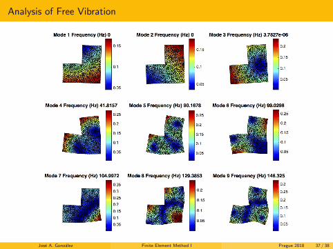
Analysis of Free Vibration
Jose A. Gonzalez Finite Element Method I Prague 2018 37 / 38

End of Lecture 6. Questions?
Jose A. Gonzalez Finite Element Method I Prague 2018 38 / 38

End of Lecture 6. Questions?
Jose A. Gonzalez Finite Element Method I Prague 2018 38 / 38