lecture 6: oligopoly - nb.vse.cznb.vse.cz/~zouharj/games/lecture_6.pdf · consider the same duopoly...

LECTURE 6:

OLIGOPOLY

Games and Decisions Jan Zouhar

Market Structures

Jan Zouhar Games and Decisions

2

the list of basic market structure types (seller-side types only):

Number of

sellers

Seller entry

barriers

Deadweight

loss

Perfect competition Many No None

Monopolistic competition Many No None

Oligopoly Few Yes Medium

Monopoly One Yes High

Collusive vs. Non-Collusive Oligopolies


3

note: oligopoly differs from monopoly (allocation-wise) only if there’s no

collusion

collusion: a largely illegal form of cooperation amongst the sellers

that includes price fixing, market division, total industry output

control, profit division, etc.

controlled by competition/anti-trust laws

well-known collusion cases: OPEC, telecommunication, drugs, sports,

chip dumping (poker)

game-theoretical models:

cooperative setting (collusive oligopoly) → coalition theory

games in the characteristic-function form

non-cooperative setting (competitive, non-collusive oligopoly) →

normal form game analysis

NE’s etc.; however, matrices can’t typically be used for payoffs

Oligopoly – Model Specification


4

to make the analysis simple, we’ll make several assumptions:

1. single-product model: oligopolists produce a single type of homogenous

product

2. one strategic variable: firms decide about prices or output levels

3. static model: single-period analysis only

in dynamic models, there are more diverse strategic options:

elimination of competitors even with contemporary losses etc.

4. single objective: all firms maximize their individual profit

Three basic non-cooperative oligopoly models:

Bertrand oligopoly – firms simultaneously choose prices

Cournot oligopoly – firms simultaneously choose quantities

Stackelberg oligopoly – firms choose quantities sequentially

note: sequential-move games are typically not modelled as normal-form

games. Instead, we use the extensive-form approach (not this lecture).

Bertrand Duopoly


5

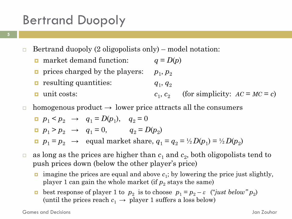
Bertrand duopoly (2 oligopolists only) – model notation:

market demand function: q = D(p)

prices charged by the players: p1, p2

resulting quantities: q1, q2

unit costs: c1, c2 (for simplicity: AC = MC = c)

homogenous product → lower price attracts all the consumers

p1 < p2 → q1 = D(p1), q2 = 0

p1 > p2 → q1 = 0, q2 = D(p2)

p1 = p2 → equal market share, q1 = q2 = ½ D(p1) = ½ D(p2)

as long as the prices are higher than c1 and c2, both oligopolists tend to

push prices down (below the other player’s price)

imagine the prices are equal and above c1; by lowering the price just slightly,

player 1 can gain the whole market (if p2 stays the same)

best response of player 1 to p2 is to choose p1 = p2 – ε (“just below” p2)

(until the prices reach c1 → player 1 suffers a loss below)

Bertrand Duopoly (cont’d)


6

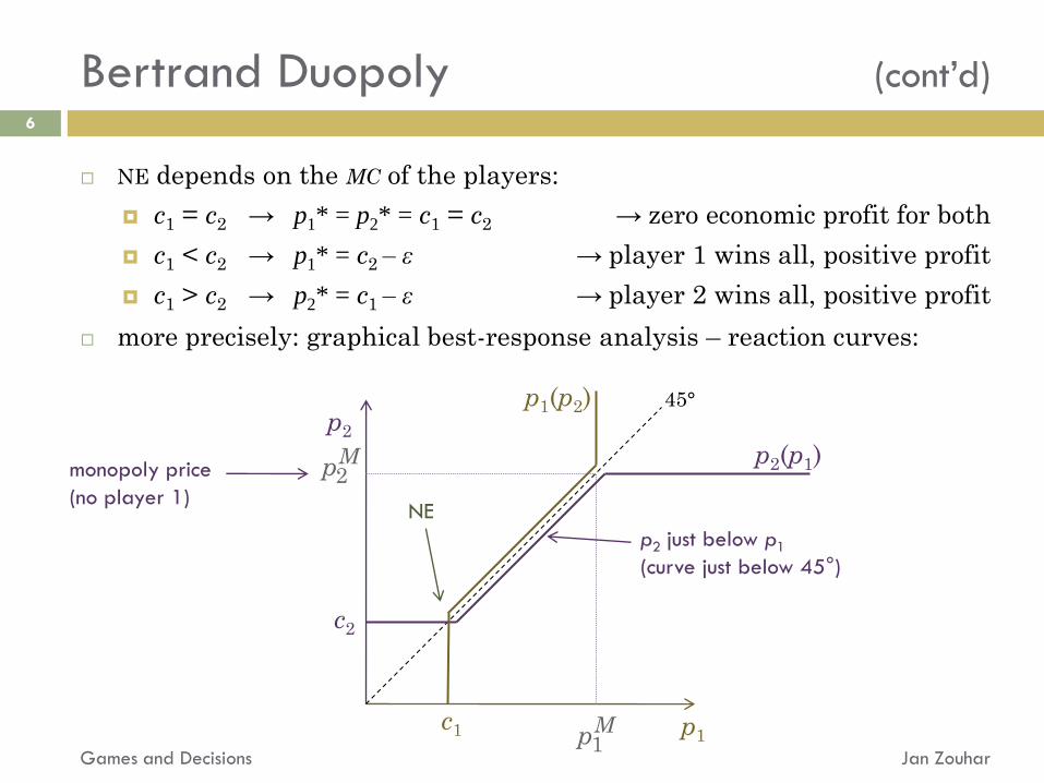
NE depends on the MC of the players:

c1 = c2 → p1* = p2* = c1 = c2 → zero economic profit for both

c1 < c2 → p1* = c2 – ε → player 1 wins all, positive profit

c1 > c2 → p2* = c1 – ε → player 2 wins all, positive profit

more precisely: graphical best-response analysis – reaction curves:

p1

p2

c1

c2

45°

p2(p1)

p1(p2)

monopoly price

(no player 1) 2Mp

1Mp

p2 just below p1

(curve just below 45°)

NE

Bertrand Duopoly (cont’d)


7

→ price competition leads to fairly efficient allocation

Critique of the Bertrand model (or, when Bertrand model fails to work)

capacity constraints of production

e.g., consider the c1 < c2 situation: if player 1 can’t supply enough for

the whole market, player 2 can still charge p2 above c2 and attract

some customers (and achieve a positive profit)

if c1 = c2 and neither player can supply to all customers, either player

can raise the output price above c

lack of product homogeneity (homogeneity disputable in most cases)

transaction/transportation costs:

may differ for the specific customer–firm interactions

e.g., shops at both ends of a street: people tend to pick the closer

one

if transportation costs are accounted for, the consumer

expenditures vary even if prices are equal

Cournot Oligopoly – Formal Treatment


8

model type – normal-form game with the following elements:

list of firms: 1,2,…,N

strategy spaces: X1, X2,…,XN

potential quantities: typically intervals

like [0,1000] → infinite alternatives!

the output level produced by ith player

(the strategy adopted) is denoted xi

a strategy profile is an N-tuple: (x1,x2,…,xN)

(where xi ∈ Xi )

cost functions: c1(x1), c2(x2),…, cN(xN)

total cost as the function of output level

price function (or inverse demand function): p = f(x1 + x2 + … + xN)

i.e., market price is the function of

total industry output

profit of ith firm: 1 1( ,..., ) ( ... ) ( )i N i i i N i ix x TR TC x f x x c x

Nash Equilibrium in Cournot Oligopoly


9

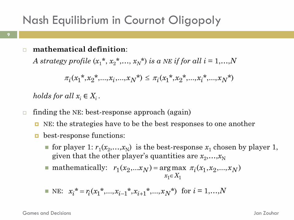
mathematical definition:

A strategy profile (x1*, x2*,…, xN*) is a NE if for all i = 1,…,N

holds for all xi ∈ Xi .

finding the NE: best-response approach (again)

NE: the strategies have to be the best responses to one another

best-response functions:

for player 1: r1(x2,…,xN) is the best-response x1 chosen by player 1,

given that the other player’s quantities are x2,…,xN

mathematically:

NE: for i = 1,…,N

1 2 1 2( *, *,..., ,..., *) ( *, *,..., *,..., *)i i N i i Nx x x x x x x x

1 1

1 2 1 2( ,... ) argmax ( , ,..., )N i Nx X

r x x x x x

1 1 1* ( *,..., *, *,..., *)i i i i Nx r x x x x

Example 1: Cournot Duopoly


10

price function:

other characteristics:

profit functions:

best response of player 1 to x2: profit-maximizing (π1-maximizing) value

of x1 for the given x2

1 2 1 2( ) 100 ( )p f x x x x

1 1 2 1 1 2 1 1

1 1 2 1

21 1 1 2

21 1 1 2

22 1 2 2 2 1 2

( , ) ( ) ( )

100 ( ) 150 12

100 150 12 1

88 150

( , ) 100 2

x x x f x x c x

x x x x

x x x x x

x x x x

x x x x x x

1 1 1 1

22 2 2 2

0, ( ) 150 12

0, ( )

X c x x

X c x x

0 20 40 60 80-2500

-2000

-1500

-1000

-500

0

500

1000

1500

x1

1

x2 = 10

x2 = 25

x2 = 50

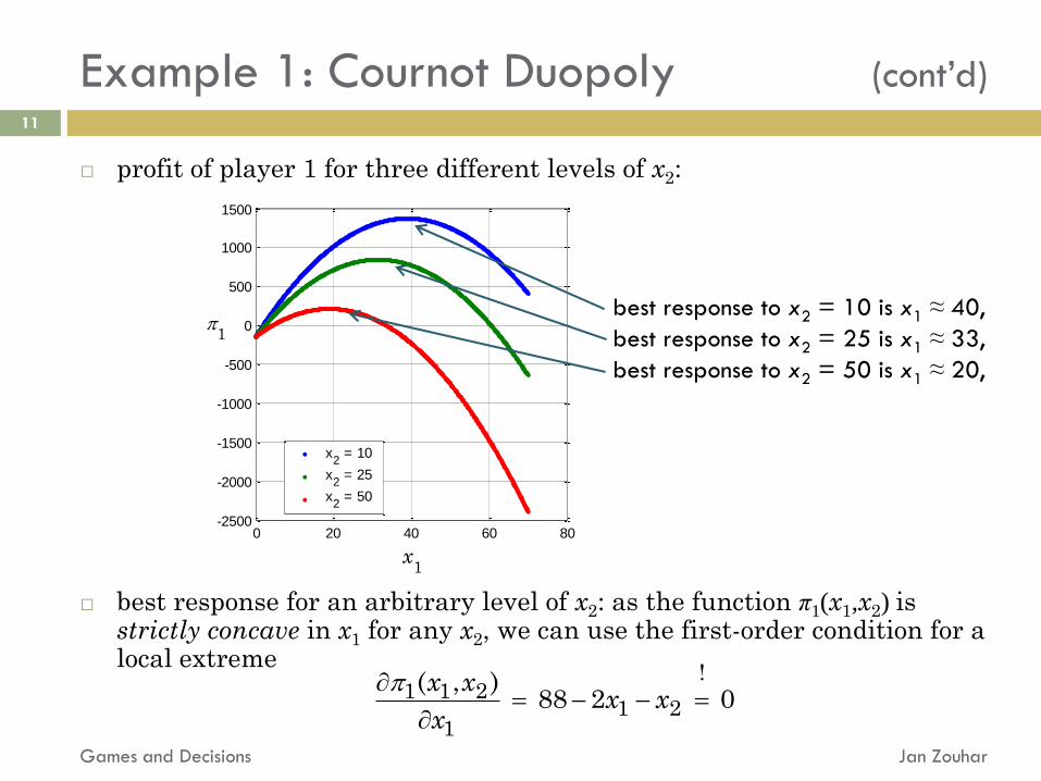
profit of player 1 for three different levels of x2:

best response for an arbitrary level of x2: as the function π1(x1,x2) is strictly concave in x1 for any x2, we can use the first-order condition for a local extreme

Example 1: Cournot Duopoly (cont’d)


11

!1 1 2

1 21

( , )88 2 0

x xx x

x

best response to x2 = 10 is x1 ≈ 40,



0 1 2 3 4 5 6 7 8 9 10-1.5

-1

-0.5

0

0.5

1

1.5

2

2.5

3


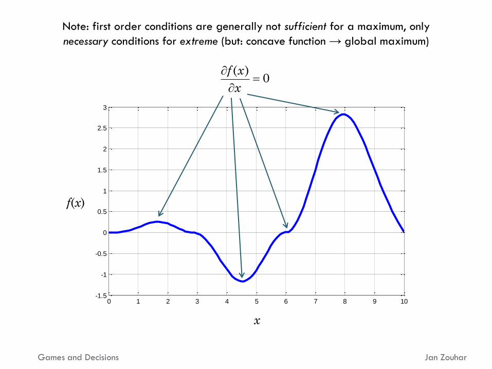
Note: first order conditions are generally not sufficient for a maximum, only

necessary conditions for extreme (but: concave function → global maximum)

f(x)

x

( )0

f x

x

Example 1: Cournot Duopoly (cont’d)


13

we can also write the result in terms of the reaction function r1:

similarly, for player 2, we obtain:

altogether, we have 2 linear equations; for NE strategies, both have to

hold at the same time → in order to find the NE, we just need to solve

1 2 1 1 2 1

1 2 2 2 1 2

88 2 * * 0 * ( *) * 36or

100 * 4 * 0 * ( *) * 16

x x x r x x

x x x r x x

1!

2 1 21 2 2 2 1 4

2

( , )100 4 0 ( ) 25

xx xx x x r x

x

2!

1 1 21 2 1 1 2 2

1

( , )88 2 0 ( ) 44

xx xx x x r x

x

Question:

What are the equilibrium profits and price?

Collusive Oligopoly


14

model framework: as in case of Cournot oligopoly, only that players can

form coalitions

coalition: a group of firms that coordinate output levels and

redistribute profits

grand coalition: the coalition of all oligopolists, Q = {1,2,…,N }

other coalitions are denoted by K,L,…

a “single-firm coalition” is still called a coalition, e.g. K = {2},

and so is the “empty coalition” {∅}

characteristic function (of the oligopoly): a function v(K) that assigns

to any coalition K the maximum attainable total profit of K

payoff function: single player, individual payoff, for a given strategy profile

characteristic function: coalition, sum of members’ profits, max. attainable

Question:

How many different coalitions can be formed with N firms?

Collusive Oligopoly (cont’d)


15

characteristic function for grand coalition:

characteristic function for other coalitions: profit of coalition members

depends on the quantity chosen by non-members

→ what will the other players do? (Generally, difficult to say.)

1. minimax characteristic function: assume non-members supply as

much as they can (up to their capacity constraints)

2. equilibrium characteristic function: assume the other players

choose the NE quantities

characteristic function for an arbitrary coalition:

1

1( ,..., ) 1

( ) max ( ,..., )N

N

i Nx x i

v Q x x

1( )

( ) max ( ,..., )i i K

i Ni Kx

v K x x

Example 2: Collusive Duopoly


16

consider the same duopoly as in example 1, only with capacity

constraints:

price function:

other characteristics:

profit functions:

first, we’ll find the equilibrium characteristic function:

we already know the NE values:

immediately, we have:

1 2 1 2( ) 100 ( )p f x x x x

1 1 1 1

22 2 2 2

0,40 ( ) 150 12

0,20 ( )

X c x x

X c x x

21 1 2 1 1 1 2

22 1 2 2 2 1 2

( , ) 88 150

( , ) 100 2

x x x x x x

x x x x x x

1 1

2 2

* 36 * 1146

* 16 * 512

x

x

1 1

2 2

1 1 1

2 2 2

(1) max ( ,16) (36,16) 1146

(2) max (36, ) (36,16) 512

x X

x X

v x

v x

Example 2: Collusive Duopoly (cont’d)


17

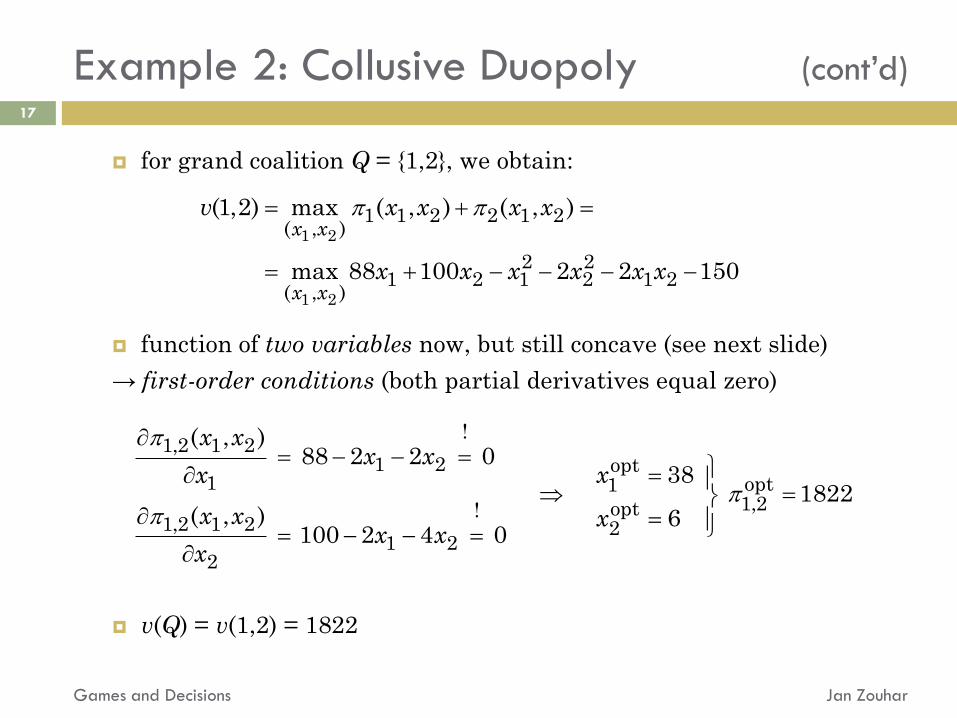
for grand coalition Q = {1,2}, we obtain:

function of two variables now, but still concave (see next slide)

→ first-order conditions (both partial derivatives equal zero)

v(Q) = v(1,2) = 1822

1 2

1 2

1 1 2 2 1 2( , )

2 21 2 1 2 1 2

( , )

(1,2) max ( , ) ( , )

max 88 100 2 2 150

x x

x x

v x x x x

x x x x x x

!1,2 1 2

1 2 opt1 opt1

1,2opt!1,2 1 2 2

1 22

( , )88 2 2 0

381822

( , ) 6100 2 4 0

x xx x

xx

x x xx x

x



-100

-50

0

50

100

-100

-50

0

50

100

-8

-6

-4

-2

0

2

x 104

x1

x2

y

-100 -50 0 50 100-100

-80

-60

-40

-20

0

20

40

60

80

100

x1

x2

π1,2


-2-1.5

-1-0.5

00.5

11.5

2

-2

-1

0

1

2

-0.5

0

0.5

x1

x2

y

first-order conditions: necessary conditions for local

extremes (not sufficient, not for maxima only!)



20

the complete equilibrium characteristic function is as follows:

minimax characteristic function:

v(∅) and v(1,2) are the same as in the equilibrium char. function

for v(1) and v(2), we calculate the players’ profits under the condition

that the other player produces up to his/her capacity constraint:

( ) 0

(1) 1146

(2) 512

(1,2) 1822

v

v

v

v

1 1 1 1

2 2 2 2

21 1 1 1

22 2 2 2 2

(1) max ( ,20) max 68 1 150 (34,20) 1006

(2) max (40, ) max 60 2 (40,15) 450

x X x X

x X x X

v x x x

v x x x



21

a comparison of the two characteristic functions:

core of the oligopoly: a division of payoffs a1,a2 such that

equilibrium minimax

v(∅) 0 0

v(1) 1146 1006

v(2) 512 450

v(1,2) 1822 1822

v(1,2) – v(1) – v(2) 164 366

1 2 1 2

1 1

2 2

1822, 1822,

1146, or 1006,

512, 450.

a a a a

a a

a a

LECTURE 6:

OLIGOPOLY

Games and Decisions Jan Zouhar

lecture 6: oligopoly - nb.vse.cznb.vse.cz/~zouharj/games/lecture_6.pdf · consider the same duopoly...

Documents