Lecture 6 : Sorting

Bong-Soo Sohn

Assistant ProfessorSchool of Computer Science and Engineering

Chung-Ang University

* Lecture notes are courtesy of F M Carrano, Prof. B-R Moon, Prof. B. McKay

2

Sorting and Efficiency Efficiency

Big O Notation Worst, best and average case performance

Simple sorting algorithms Selection sort Bubblesort Insertion Sort

Partitioning Algorithms Merge Sort Quicksort

Radix Sort

3

Algorithm Efficiency & Sorting

O( ): Big-Oh An algorithm is said to take O(f (n)) if its running time is upper-bounded by cf(n) e.g., O(n), O(n log n), O(n2), O(2n), …

Formal definition O(f(n)) = { g(n) | ∃c > 0, n0 ≥ 0 s.t.∀n ≥ n0, cf(n) ≥ g(n) } g(n) ∈ O(f(n)) 이 맞지만 관행적으로 g(n) = O(f(n)) 이라고 쓴다 .

직관적 의미 g(n) = O(f(n)) ⇒ g grows no faster than f

4

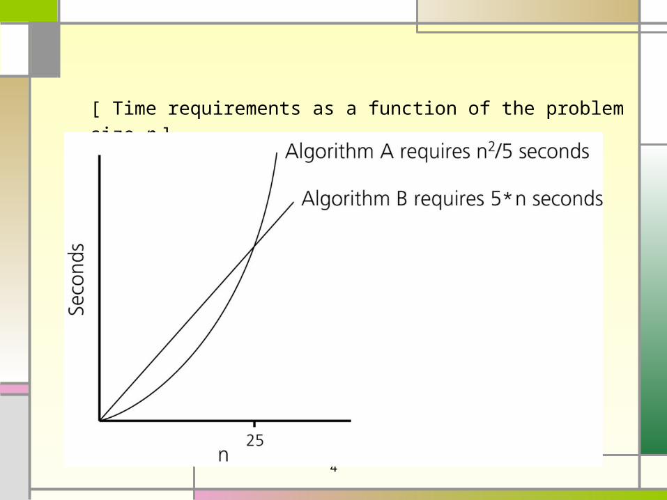
[ Time requirements as a function of the problem size n ]

5

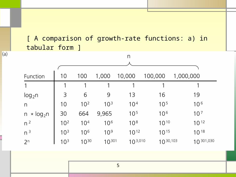
[ A comparison of growth-rate functions: a) in tabular form ]

6

[ A comparison of growth-rate functions: b) in graphical form ]

7

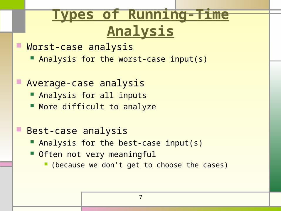
Types of Running-Time Analysis

Worst-case analysis Analysis for the worst-case input(s)

Average-case analysis Analysis for all inputs More difficult to analyze

Best-case analysis Analysis for the best-case input(s) Often not very meaningful

(because we don’t get to choose the cases)

8

Running Time for Search in an Array

Sequential search Worst case: O(n) Average case: O(n) Best case: O(1)

Binary search Worst case: O(log n) Average case: O(log n) Best case: O(1)

9

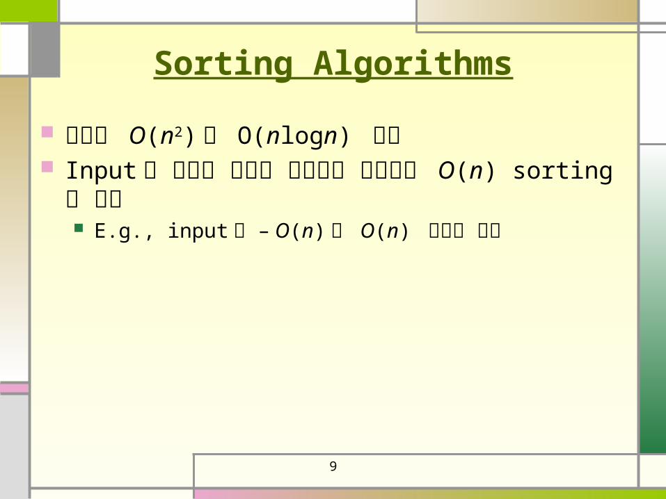
Sorting Algorithms

대부분 O(n2) 과 O(nlogn) 사이 Input 이 특수한 성질을 만족하는 경우에는 O(n)

sorting 도 가능 E.g., input 이 – O(n) 과 O(n) 사이의 정수

10

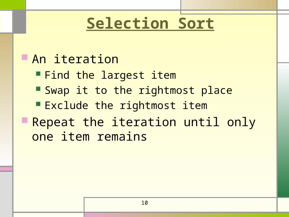
Selection Sort

An iteration Find the largest item Swap it to the rightmost place Exclude the rightmost item

Repeat the iteration until only one item remains

11

The largest itemThe largest item

Running time: (n-1)+(n-2)+···+2+1 = O(n2)Worst caseAverage case

12

selectionSort(theArray[ ], n)

{

for (last = n-1; last >=1; last--) {

largest = indexOfLargest(theArray, last+1);

Swap theArray[largest] & theArray[last];

}

}

indexOfLargest(theArray, size)

{

largest = 0;

for (i = 1; i < size; ++i) {

if (theArray[i] > theArray[largest]) largest = i;

}

}

(n-1)+(n-2)+···+2+1 = O(n2)

The loop in selectionSort calls indexOfLargest n times

Each call to IndexOfLargest creates a loop of 1 less time than the previous

13

Bubble Sort

Running time: (n-1)+(n-2)+···+2+1 = O(n2)Worst caseAverage case

14

Insertion Sort

Running time: O(n2)Worst case: 1+2+···+(n-2)+(n-1)Average case: ½ (1+2+···+(n-2)+(n-1))

15

[ An insertion sort partitions the array into two regions ]

16

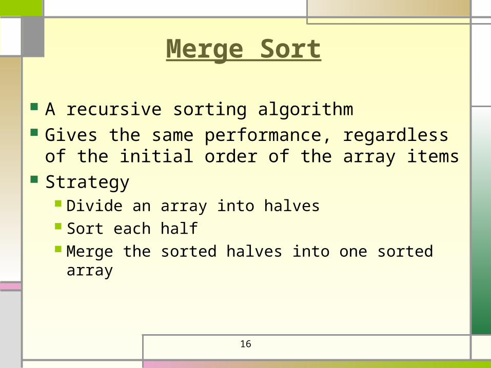
Merge Sort

A recursive sorting algorithm Gives the same performance, regardless of the

initial order of the array items Strategy

Divide an array into halves Sort each half Merge the sorted halves into one sorted array

17

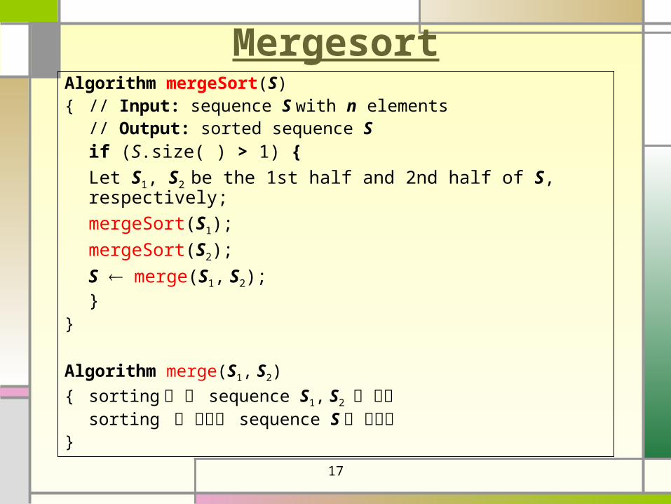
MergesortAlgorithm mergeSort(S){ // Input: sequence S with n elements

// Output: sorted sequence S

if (S.size( ) > 1) {

Let S1, S2 be the 1st half and 2nd half of S, respectively;

mergeSort(S1);

mergeSort(S2);

S merge(S1, S2);}

}

Algorithm merge(S1, S2)

{ sorting 된 두 sequence S1, S2 를 합쳐 sorting 된 하나의 sequence S 를 만든다

}

18

7 2 | 9 4

7 | 2

7 2 9 4 3 8 6 1

7

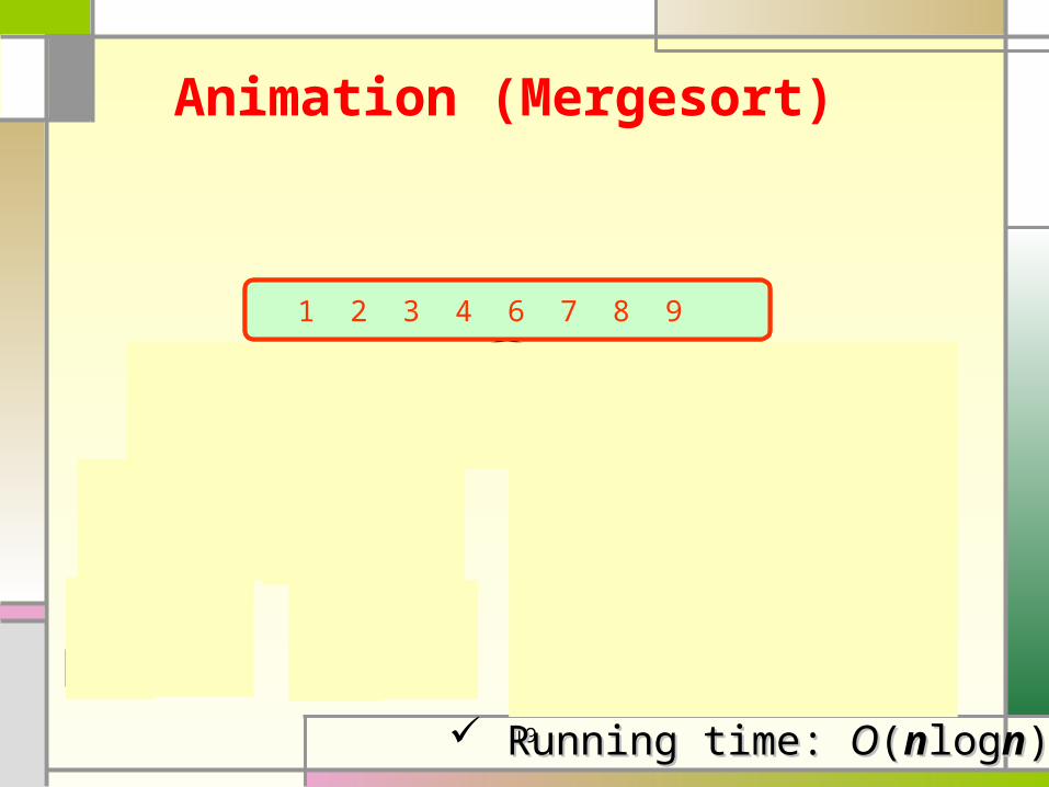
Animation (Mergesort)

19

9 | 4

7 2 | 9 4

7 | 2

7 2 9 4 3 8 6 1

7

7

2

22 7

2 7

9 4

9 44 9

4 92 4 7 9

1 3 6 82 4 7 91 2 3 4 6 7 8 9

Animation (Mergesort)

Running time: Running time: OO((nnloglognn))

20

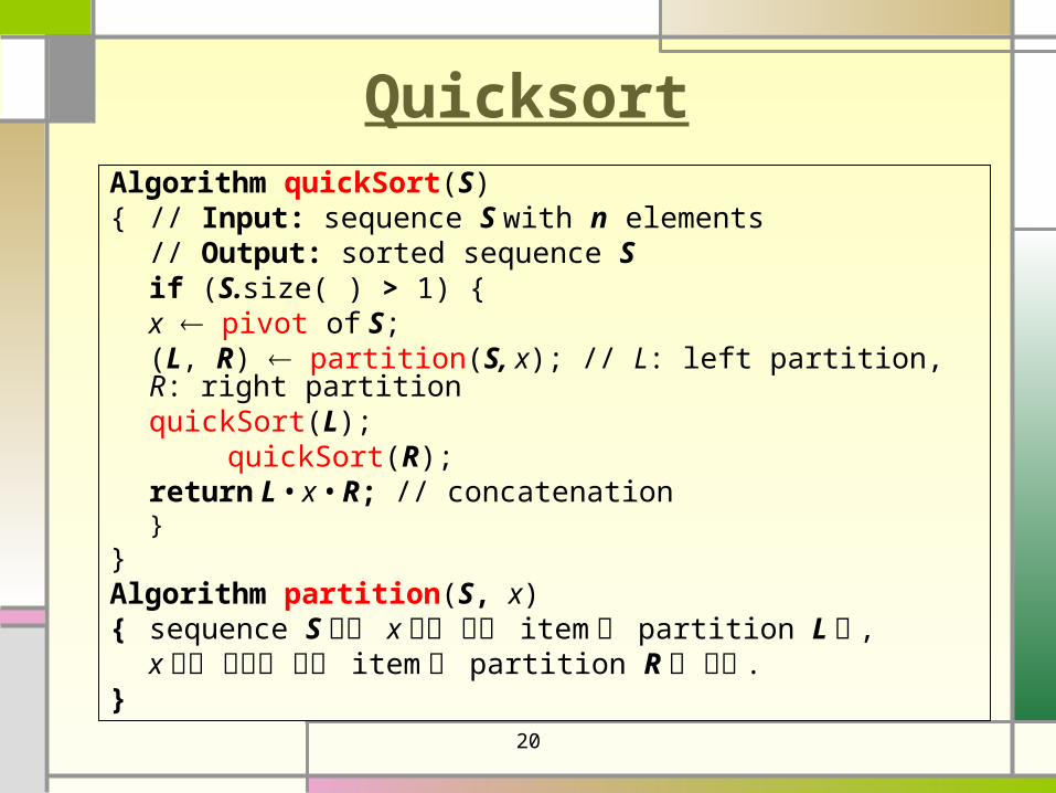
QuicksortAlgorithm quickSort(S){ // Input: sequence S with n elements

// Output: sorted sequence Sif (S.size( ) > 1) {

x pivot of S; (L, R) partition(S, x); // L: left partition, R: right partitionquickSort(L);

quickSort(R);return L • x • R; // concatenation

}}Algorithm partition(S, x){ sequence S 에서 x 보다 작은 item 은 partition L 로 ,

x 보다 크거나 같은 item 은 partition R 로 분류 .}

21

1 1

5 1 9 4 2 6 8 3

Animation (Quicksort)

3 1 4 2 5 9 6 8

2 1

3 1 4 22 1 3 4

1 2

1 1

1 2 44

1 2

1 2 3 41 2 3 4

1 2 3 4 5 9 6 8

9 6 8

8 6

6

8 6 9

6 8

6

6 86 8

6 8 96 8 9

1 2 3 4 5 6 8 9

Average-case running time: Average-case running time: OO((nnloglognn)) Worst-case running time: Worst-case running time: OO((nn22))

22

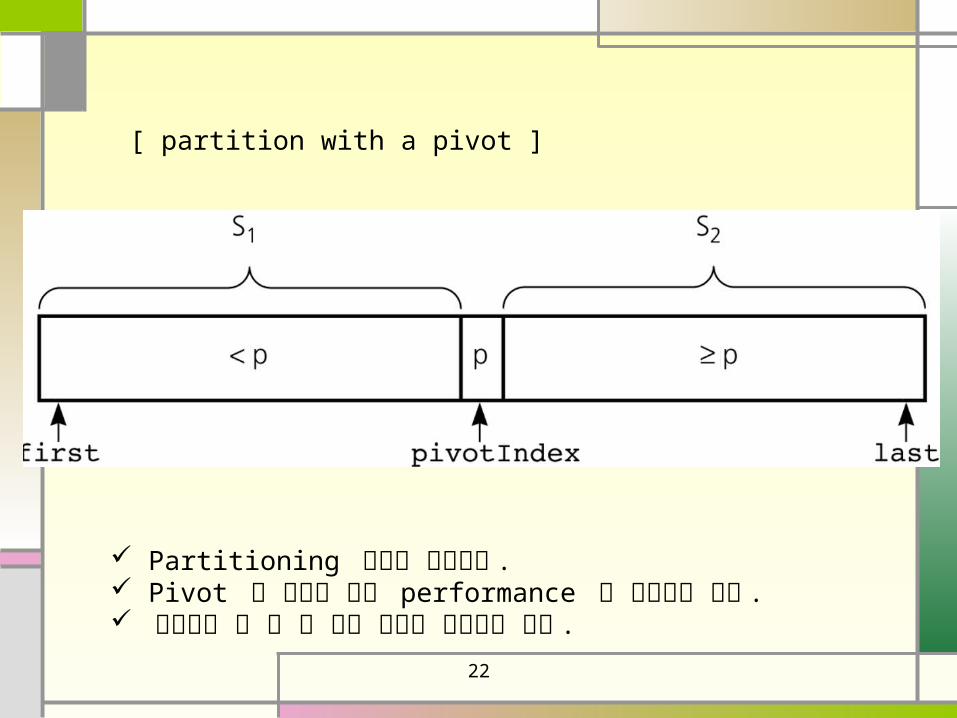
[ partition with a pivot ]

Partitioning 방법은 다양하다 . Pivot 의 선택에 따라 performance 가 달라질수 있다 . 교과서에 그 중 한 가지 방법을 소개하고 있다 .

23

Stable and Deterministic Sorting A sort algorithm must sort the elements into order But what happens to elements which are equal? Stable sort

Elements are in the same order as the original sequence Eg merge-sort

Deterministic Sort Elements are always in the same order

Non-deterministic example Quicksort with random pivot

Stable deterministic But not vice versa

24

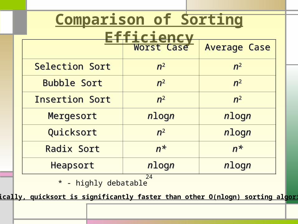
Comparison of Sorting Efficiency

Worst CaseWorst Case Average CaseAverage Case

Selection SortSelection Sort nn22 nn22

Bubble SortBubble Sort nn22 nn22

Insertion SortInsertion Sort nn22 nn22

MergesortMergesort nnloglognn nnloglognn

QuicksortQuicksort nn22 nnloglognn

Radix SortRadix Sort n*n* n*n*

HeapsortHeapsort nnloglognn nnloglognn

* - highly debatable

• Typically, quicksort is significantly faster than other O(nlogn) sorting algorithms

25

Summary Efficiency

Big O Notation Worst, best and average case

performance Simple sorting algorithms

Selection sort Bubblesort Insertion Sort

Partitioning Algorithms Merge Sort Quicksort