lecture 7: hardware acceleration of dnns
TRANSCRIPT

Visual Computing Systems Stanford CS348K, Spring 2021
Lecture 7:
Hardware Acceleration of DNNs

Stanford CS348K, Spring 2021
Hardware acceleration of DNN inference/training
Google TPU3
Huawei Kirin NPU
Apple Neural Engine
GraphCore IPU
Ampere GPU with Tensor Cores
Intel Deep Learning Inference Accelerator
Cerebras Wafer Scale Engine
SambaNova Cardinal SN10

Stanford CS348K, Spring 2021
Investment in AI hardware
NVIDIA Market Cap 2014 - 2021

Stanford CS348K, Spring 2021
Two computer architecture reminders
Stanford CS348K, Spring 2021
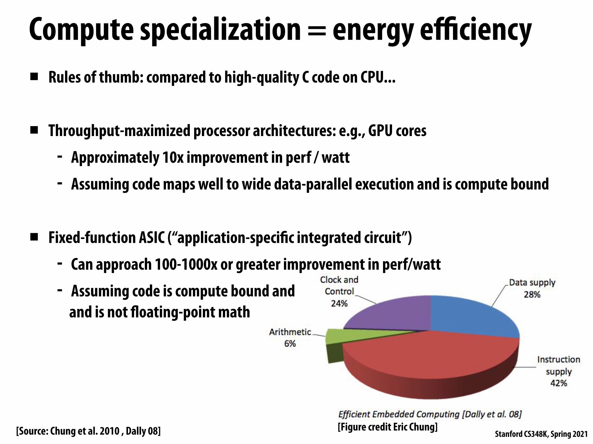
Compute specialization = energy e!ciency▪ Rules of thumb: compared to high-quality C code on CPU...
▪ Throughput-maximized processor architectures: e.g., GPU cores - Approximately 10x improvement in perf / watt - Assuming code maps well to wide data-parallel execution and is compute bound
▪ Fixed-function ASIC (“application-speci"c integrated circuit”) - Can approach 100-1000x or greater improvement in perf/watt - Assuming code is compute bound and
and is not #oating-point math
[Source: Chung et al. 2010 , Dally 08] [Figure credit Eric Chung]

Stanford CS348K, Spring 2021
Data movement has high energy cost▪ Rule of thumb in modern system design: always seek to reduce amount of
data movement in a computer
▪ “Ballpark” numbers - Integer op: ~ 1 pJ * - Floating point op: ~20 pJ * - Reading 64 bits from small local SRAM (1mm away on chip): ~ 26 pJ - Reading 64 bits from low power mobile DRAM (LPDDR): ~1200 pJ
▪ Implications - Reading 10 GB/sec from memory: ~1.6 watts - Entire power budget for mobile GPU: ~1 watt
(remember phone is also running CPU, display, radios, etc.) - iPhone 6 battery: ~7 watt-hours (note: my Macbook Pro laptop: 99 watt-hour battery) - Exploiting locality matters!!!
* Cost to just perform the logical operation, not counting overhead of instruction decode, load data from registers, etc.
[Sources: Bill Dally (NVIDIA), Tom Olson (ARM)]

Stanford CS348K, Spring 2021
On-chip caches locate data near processingProcessors run e!ciently when data is resident in caches
Caches reduce memory access latency * Caches reduce the energy cost of data access
38 GB/secL3 cache
(8 MB)
L1 cache (32 KB)
L2 cache (256 KB)
L1 cache (32 KB)
L2 cache (256 KB)
. . .
Memory DDR4 DRAM
(Gigabytes)
Core 1
Core N
* Caches also provide high bandwidth data transfer to CPU

Stanford CS348K, Spring 2021
Example: NVIDIA A100 GPU
Up to 80 GB HMB2 stacked memory 2 TB/sec memory bandwidth
Also note: A100 has 40 MB L2 cache (increased from 6.1 MB on V100)
Memory stacking locates memory near chip

Stanford CS348K, Spring 2021
Improving hardware e!ciency for DNN operations

Stanford CS348K, Spring 2021
Amortize overhead of instruction stream control using more complex instructions
▪ Fused multiply add (ax + b) ▪ 4-component dot product x = A dot B ▪ 4x4 matrix multiply
- AB + C for 4x4 matrices A, B, C
▪ Key principle: amortize cost of instruction stream processing across many operations of a single complex instruction
Stanford CS348K, Spring 2021
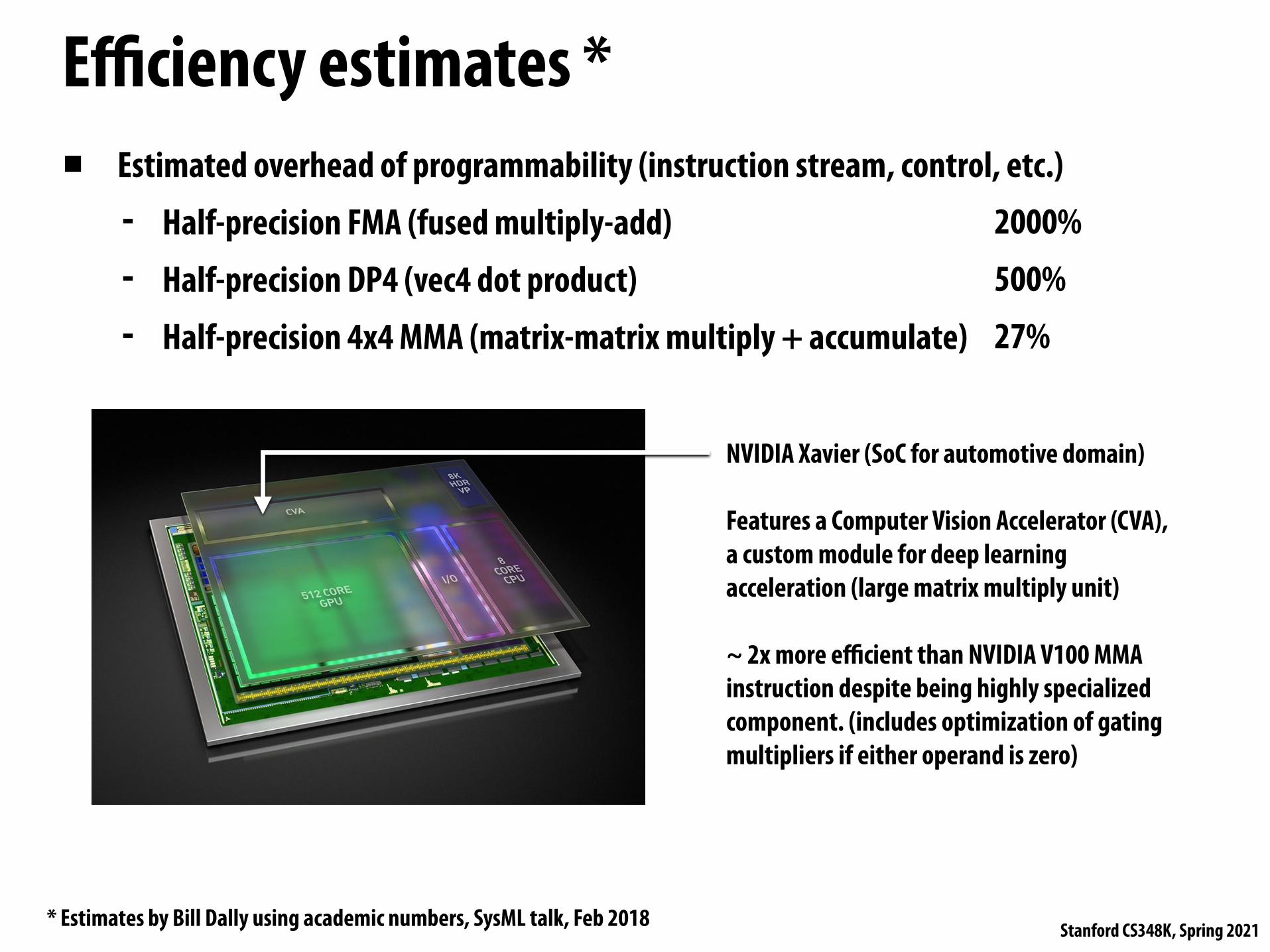
E!ciency estimates *▪ Estimated overhead of programmability (instruction stream, control, etc.)
- Half-precision FMA (fused multiply-add) - Half-precision DP4 (vec4 dot product) - Half-precision 4x4 MMA (matrix-matrix multiply + accumulate)
2000% 500% 27%
NVIDIA Xavier (SoC for automotive domain)
Features a Computer Vision Accelerator (CVA), a custom module for deep learning acceleration (large matrix multiply unit)
~ 2x more e!cient than NVIDIA V100 MMA instruction despite being highly specialized component. (includes optimization of gating multipliers if either operand is zero)
* Estimates by Bill Dally using academic numbers, SysML talk, Feb 2018
Stanford CS348K, Spring 2021
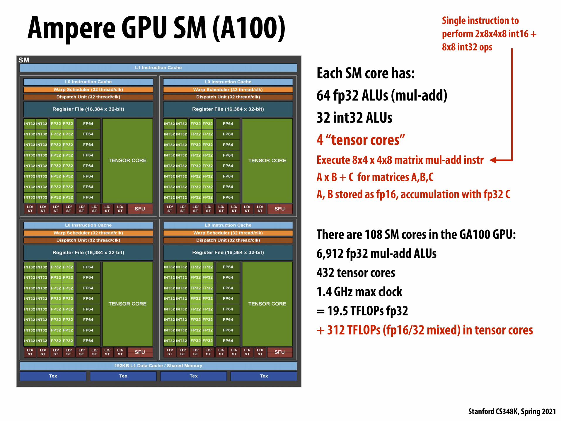
Ampere GPU SM (A100)Each SM core has: 64 fp32 ALUs (mul-add) 32 int32 ALUs 4 “tensor cores” Execute 8x4 x 4x8 matrix mul-add instr A x B + C for matrices A,B,C A, B stored as fp16, accumulation with fp32 C
There are 108 SM cores in the GA100 GPU: 6,912 fp32 mul-add ALUs 432 tensor cores 1.4 GHz max clock = 19.5 TFLOPs fp32 + 312 TFLOPs (fp16/32 mixed) in tensor cores
Single instruction to perform 2x8x4x8 int16 + 8x8 int32 ops

Stanford CS348K, Spring 2021
Google TPU (version 1)
Stanford CS348K, Spring 2021
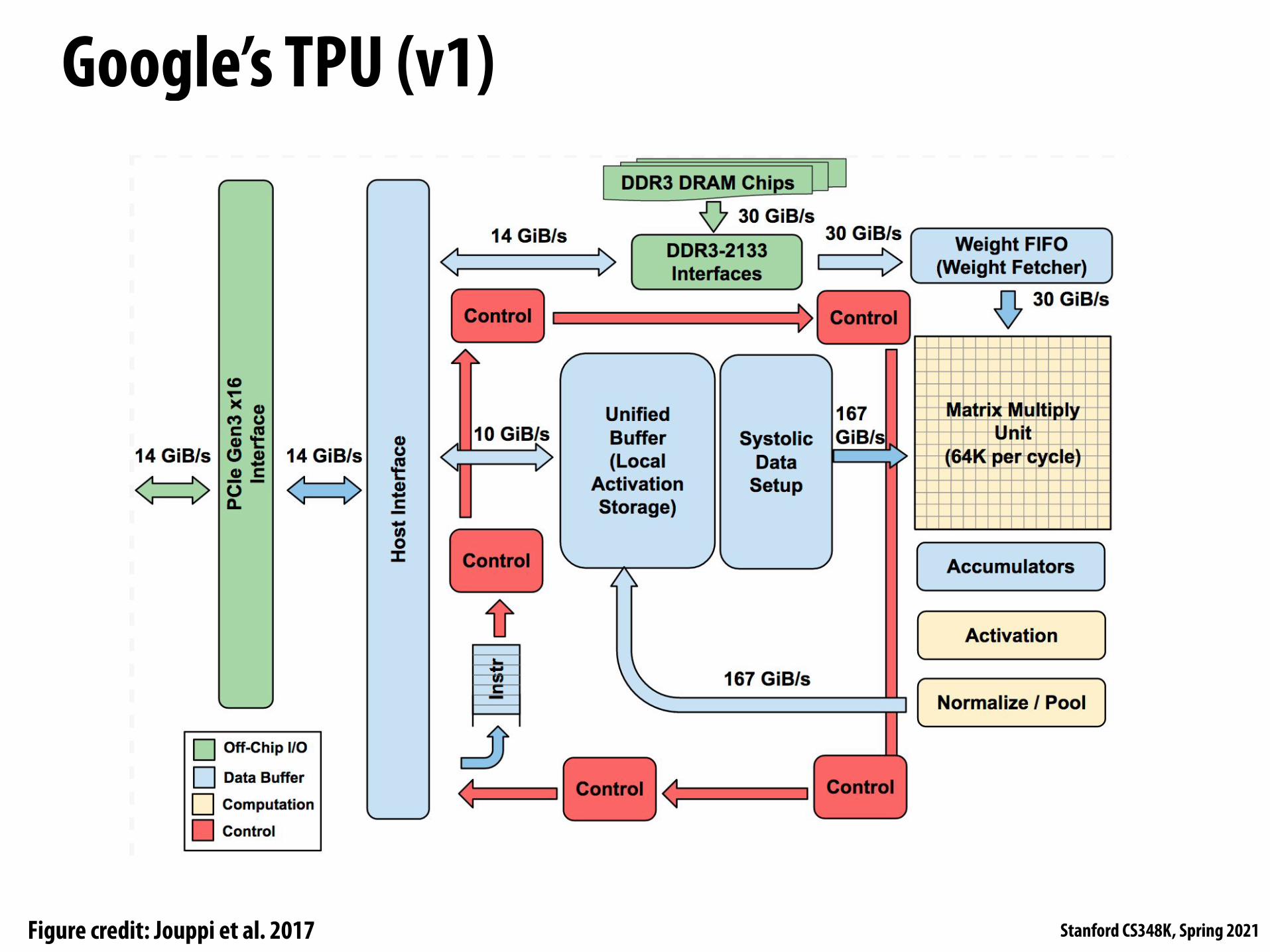
Google’s TPU (v1)
Hence, the TPU is closer in spirit to an FPU (floating-point unit) coprocessor than it is to a GPU.
Figure 1. TPU Block Diagram. The main computation part is the Figure 2. Floor Plan of TPU die. The shading follows Figure 1. yellow Matrix Multiply unit in the upper right hand corner. Its inputs The light (blue) data buffers are 37% of the die, the light (yellow) are the blue Weight FIFO and the blue Unified Buffer (UB) and its compute is 30%, the medium (green) I/O is 10%, and the dark output is the blue Accumulators (Acc). The yellow Activation Unit (red) control is just 2%. Control is much larger (and much more performs the nonlinear functions on the Acc, which go to the UB. difficult to design) in a CPU or GPU
The goal was to run whole inference models in the TPU to reduce interactions with the host CPU and to be flexible enough to match the NN needs of 2015 and beyond, instead of just what was required for 2013 NNs. Figure 1 shows the block diagram of the TPU.
The TPU instructions are sent from the host over the PCIe Gen3 x16 bus into an instruction buffer. The internal blocks are typically connected together by 256-byte -wide paths. Starting in the upper-right corner, the Matrix Multiply Unit is the heart of the TPU. It contains 256x256 MACs that can perform 8-bit multiply-and-adds on signed or unsigned integers. The 16-bit products are collected in the 4 MiB of 32-bit Accumulators below the matrix unit. The 4MiB represents 4096, 256-element, 32-bit accumulators. The matrix unit produces one 256-element partial sum per clock cycle. We picked 4096 by first noting that the operations per byte need to reach peak performance (roofline knee in Section 4) is ~1350, so we rounded that up to 2048 and then duplicated it so that the compiler could use double buffering while running at peak performance.
When using a mix of 8-bit weights and 16-bit activations (or vice versa), the Matrix Unit computes at half-speed, and it computes at a quarter-speed when both are 16 bits. It reads and writes 256 values per clock cycle and can perform either a matrix multiply or a convolution. The matrix unit holds one 64 KiB tile of weights plus one for double-buffering (to hide the 256 cycles it takes to shift a tile in). This unit is designed for dense matrices. Sparse architectural support was omitted for time-to-deploy reasons. Sparsity will have high priority in future designs.
The weights for the matrix unit are staged through an on-chip Weight FIFO that reads from an off-chip 8 GiB DRAM called Weight Memory (for inference, weights are read-only; 8 GiB supports many simultaneously active models). The weight FIFO is four tiles deep. The intermediate results are held in the 24 MiB on-chip Unified Buffer , which can serve as inputs to the Matrix Unit. A programmable DMA controller transfers data to or from CPU Host memory and the Unified Buffer.
Figure 2 shows the floor plan of the TPU die. The 24 MiB Unified Buffer is almost a third of the die and the Matrix Multiply Unit is a quarter, so the datapath is nearly two-thirds of the die. The 24 MiB size was picked in part to match the pitch of the Matrix Unit on the die and, given the short development schedule, in part to simplify the compiler (see Section 7). Control is just 2%. Figure 3 shows the TPU on its printed circuit card, which inserts into existing servers like an SATA disk.
As instructions are sent over the relatively slow PCIe bus, TPU instructions follow the CISC tradition, including a repeat field. The average clock cycles per instruction (CPI) of these CISC instructions is typically 10 to 20. It has about a dozen instructions overall, but these five are the key ones:
1. Read_Host_Memory reads data from the CPU host memory into the Unified Buffer (UB). 2. Read_Weights reads weights from Weight Memory into the Weight FIFO as input to the Matrix Unit. 3. MatrixMultiply/Convolve causes the Matrix Unit to perform a matrix multiply or a convolution from the
Unified Buffer into the Accumulators. A matrix operation takes a variable-sized B*256 input, multiplies it by a 256x256 constant weight input, and produces a B*256 output, taking B pipelined cycles to complete.
3
Figure credit: Jouppi et al. 2017

Stanford CS348K, Spring 2021
TPU area proportionality
Hence, the TPU is closer in spirit to an FPU (floating-point unit) coprocessor than it is to a GPU.
Figure 1. TPU Block Diagram. The main computation part is the Figure 2. Floor Plan of TPU die. The shading follows Figure 1. yellow Matrix Multiply unit in the upper right hand corner. Its inputs The light (blue) data buffers are 37% of the die, the light (yellow) are the blue Weight FIFO and the blue Unified Buffer (UB) and its compute is 30%, the medium (green) I/O is 10%, and the dark output is the blue Accumulators (Acc). The yellow Activation Unit (red) control is just 2%. Control is much larger (and much more performs the nonlinear functions on the Acc, which go to the UB. difficult to design) in a CPU or GPU
The goal was to run whole inference models in the TPU to reduce interactions with the host CPU and to be flexible enough to match the NN needs of 2015 and beyond, instead of just what was required for 2013 NNs. Figure 1 shows the block diagram of the TPU.
The TPU instructions are sent from the host over the PCIe Gen3 x16 bus into an instruction buffer. The internal blocks are typically connected together by 256-byte -wide paths. Starting in the upper-right corner, the Matrix Multiply Unit is the heart of the TPU. It contains 256x256 MACs that can perform 8-bit multiply-and-adds on signed or unsigned integers. The 16-bit products are collected in the 4 MiB of 32-bit Accumulators below the matrix unit. The 4MiB represents 4096, 256-element, 32-bit accumulators. The matrix unit produces one 256-element partial sum per clock cycle. We picked 4096 by first noting that the operations per byte need to reach peak performance (roofline knee in Section 4) is ~1350, so we rounded that up to 2048 and then duplicated it so that the compiler could use double buffering while running at peak performance.
When using a mix of 8-bit weights and 16-bit activations (or vice versa), the Matrix Unit computes at half-speed, and it computes at a quarter-speed when both are 16 bits. It reads and writes 256 values per clock cycle and can perform either a matrix multiply or a convolution. The matrix unit holds one 64 KiB tile of weights plus one for double-buffering (to hide the 256 cycles it takes to shift a tile in). This unit is designed for dense matrices. Sparse architectural support was omitted for time-to-deploy reasons. Sparsity will have high priority in future designs.
The weights for the matrix unit are staged through an on-chip Weight FIFO that reads from an off-chip 8 GiB DRAM called Weight Memory (for inference, weights are read-only; 8 GiB supports many simultaneously active models). The weight FIFO is four tiles deep. The intermediate results are held in the 24 MiB on-chip Unified Buffer , which can serve as inputs to the Matrix Unit. A programmable DMA controller transfers data to or from CPU Host memory and the Unified Buffer.
Figure 2 shows the floor plan of the TPU die. The 24 MiB Unified Buffer is almost a third of the die and the Matrix Multiply Unit is a quarter, so the datapath is nearly two-thirds of the die. The 24 MiB size was picked in part to match the pitch of the Matrix Unit on the die and, given the short development schedule, in part to simplify the compiler (see Section 7). Control is just 2%. Figure 3 shows the TPU on its printed circuit card, which inserts into existing servers like an SATA disk.
As instructions are sent over the relatively slow PCIe bus, TPU instructions follow the CISC tradition, including a repeat field. The average clock cycles per instruction (CPI) of these CISC instructions is typically 10 to 20. It has about a dozen instructions overall, but these five are the key ones:
1. Read_Host_Memory reads data from the CPU host memory into the Unified Buffer (UB). 2. Read_Weights reads weights from Weight Memory into the Weight FIFO as input to the Matrix Unit. 3. MatrixMultiply/Convolve causes the Matrix Unit to perform a matrix multiply or a convolution from the
Unified Buffer into the Accumulators. A matrix operation takes a variable-sized B*256 input, multiplies it by a 256x256 constant weight input, and produces a B*256 output, taking B pipelined cycles to complete.
3
Arithmetic units ~ 30% of chip Note low area footprint of control
Key instructions: read host memory write host memory read weights matrix_multiply / convolve activate
Hence, the TPU is closer in spirit to an FPU (floating-point unit) coprocessor than it is to a GPU.
Figure 1. TPU Block Diagram. The main computation part is the Figure 2. Floor Plan of TPU die. The shading follows Figure 1. yellow Matrix Multiply unit in the upper right hand corner. Its inputs The light (blue) data buffers are 37% of the die, the light (yellow) are the blue Weight FIFO and the blue Unified Buffer (UB) and its compute is 30%, the medium (green) I/O is 10%, and the dark output is the blue Accumulators (Acc). The yellow Activation Unit (red) control is just 2%. Control is much larger (and much more performs the nonlinear functions on the Acc, which go to the UB. difficult to design) in a CPU or GPU
The goal was to run whole inference models in the TPU to reduce interactions with the host CPU and to be flexible enough to match the NN needs of 2015 and beyond, instead of just what was required for 2013 NNs. Figure 1 shows the block diagram of the TPU.
The TPU instructions are sent from the host over the PCIe Gen3 x16 bus into an instruction buffer. The internal blocks are typically connected together by 256-byte -wide paths. Starting in the upper-right corner, the Matrix Multiply Unit is the heart of the TPU. It contains 256x256 MACs that can perform 8-bit multiply-and-adds on signed or unsigned integers. The 16-bit products are collected in the 4 MiB of 32-bit Accumulators below the matrix unit. The 4MiB represents 4096, 256-element, 32-bit accumulators. The matrix unit produces one 256-element partial sum per clock cycle. We picked 4096 by first noting that the operations per byte need to reach peak performance (roofline knee in Section 4) is ~1350, so we rounded that up to 2048 and then duplicated it so that the compiler could use double buffering while running at peak performance.
When using a mix of 8-bit weights and 16-bit activations (or vice versa), the Matrix Unit computes at half-speed, and it computes at a quarter-speed when both are 16 bits. It reads and writes 256 values per clock cycle and can perform either a matrix multiply or a convolution. The matrix unit holds one 64 KiB tile of weights plus one for double-buffering (to hide the 256 cycles it takes to shift a tile in). This unit is designed for dense matrices. Sparse architectural support was omitted for time-to-deploy reasons. Sparsity will have high priority in future designs.
The weights for the matrix unit are staged through an on-chip Weight FIFO that reads from an off-chip 8 GiB DRAM called Weight Memory (for inference, weights are read-only; 8 GiB supports many simultaneously active models). The weight FIFO is four tiles deep. The intermediate results are held in the 24 MiB on-chip Unified Buffer , which can serve as inputs to the Matrix Unit. A programmable DMA controller transfers data to or from CPU Host memory and the Unified Buffer.
Figure 2 shows the floor plan of the TPU die. The 24 MiB Unified Buffer is almost a third of the die and the Matrix Multiply Unit is a quarter, so the datapath is nearly two-thirds of the die. The 24 MiB size was picked in part to match the pitch of the Matrix Unit on the die and, given the short development schedule, in part to simplify the compiler (see Section 7). Control is just 2%. Figure 3 shows the TPU on its printed circuit card, which inserts into existing servers like an SATA disk.
As instructions are sent over the relatively slow PCIe bus, TPU instructions follow the CISC tradition, including a repeat field. The average clock cycles per instruction (CPI) of these CISC instructions is typically 10 to 20. It has about a dozen instructions overall, but these five are the key ones:
1. Read_Host_Memory reads data from the CPU host memory into the Unified Buffer (UB). 2. Read_Weights reads weights from Weight Memory into the Weight FIFO as input to the Matrix Unit. 3. MatrixMultiply/Convolve causes the Matrix Unit to perform a matrix multiply or a convolution from the
Unified Buffer into the Accumulators. A matrix operation takes a variable-sized B*256 input, multiplies it by a 256x256 constant weight input, and produces a B*256 output, taking B pipelined cycles to complete.
3
Figure credit: Jouppi et al. 2017

Stanford CS348K, Spring 2021
Systolic array (matrix vector multiplication example: y=Wx)
PE PE PE PE
PE PE PE PE
PE PE PE PE
PE PE PE PE
Accumulators (32-bit)
+ + + +
Weights FIFO
w00
w01
w02
w03
w10
w11
w12
w13
w20
w21
w22
w23
w30
w31
w32
w33

Stanford CS348K, Spring 2021
Systolic array (matrix vector multiplication example: y=Wx)
PE PE PE PE
PE PE PE PE
PE PE PE PE
PE PE PE PE
Accumulators (32-bit)
+ + + +
Weights FIFO
w00
w01
w02
w03
w10
w11
w12
w13
w20
w21
w22
w23
w30
w31
w32
w33
x0

Stanford CS348K, Spring 2021
Systolic array (matrix vector multiplication example: y=Wx)
PE PE PE PE
PE PE PE PE
PE PE PE PE
PE PE PE PE
Accumulators (32-bit)
+ + + +
Weights FIFO
w00
w01
w02
w03
w10
w11
w12
w13
w20
w21
w22
w23
w30
w31
w32
w33
x0 * w00
x1
x0

Stanford CS348K, Spring 2021
Systolic array (matrix vector multiplication example: y=Wx)
PE PE PE PE
PE PE PE PE
PE PE PE PE
PE PE PE PE
Accumulators (32-bit)
+ + + +
Weights FIFO
w00
w01
w02
w03
w10
w11
w12
w13
w20
w21
w22
w23
w30
w31
w32
w33
x2
x0
x0 * w10
x0 * w00 + x1 * w01
x1

Stanford CS348K, Spring 2021
Systolic array (matrix vector multiplication example: y=Wx)
PE PE PE PE
PE PE PE PE
PE PE PE PE
PE PE PE PE
Accumulators (32-bit)
+ + + +
Weights FIFO
w00
w01
w02
w03
w10
w11
w12
w13
w20
w21
w22
w23
w30
w31
w32
w33
x2
x0
x0 * w00 + x1 * w01 + x2 * w02 +
x3
x1
x0 * w10 + x1 * w11
x0 * w20

Stanford CS348K, Spring 2021
Systolic array (matrix vector multiplication example: y=Wx)
PE PE PE PE
PE PE PE PE
PE PE PE PE
PE PE PE PE
Accumulators (32-bit)
+ + + +
Weights FIFO
w00
w01
w02
w03
w10
w11
w12
w13
w20
w21
w22
w23
w30
w31
w32
w33
x2
x0 * w10 + x1 * w11 + x2 * w12 +
x3
x1
x0 * w20 + x1 * w21
x0 * w30
x0 * w00 + x1 * w01 + x2 * w02 + x3 * w03
Stanford CS348K, Spring 2021
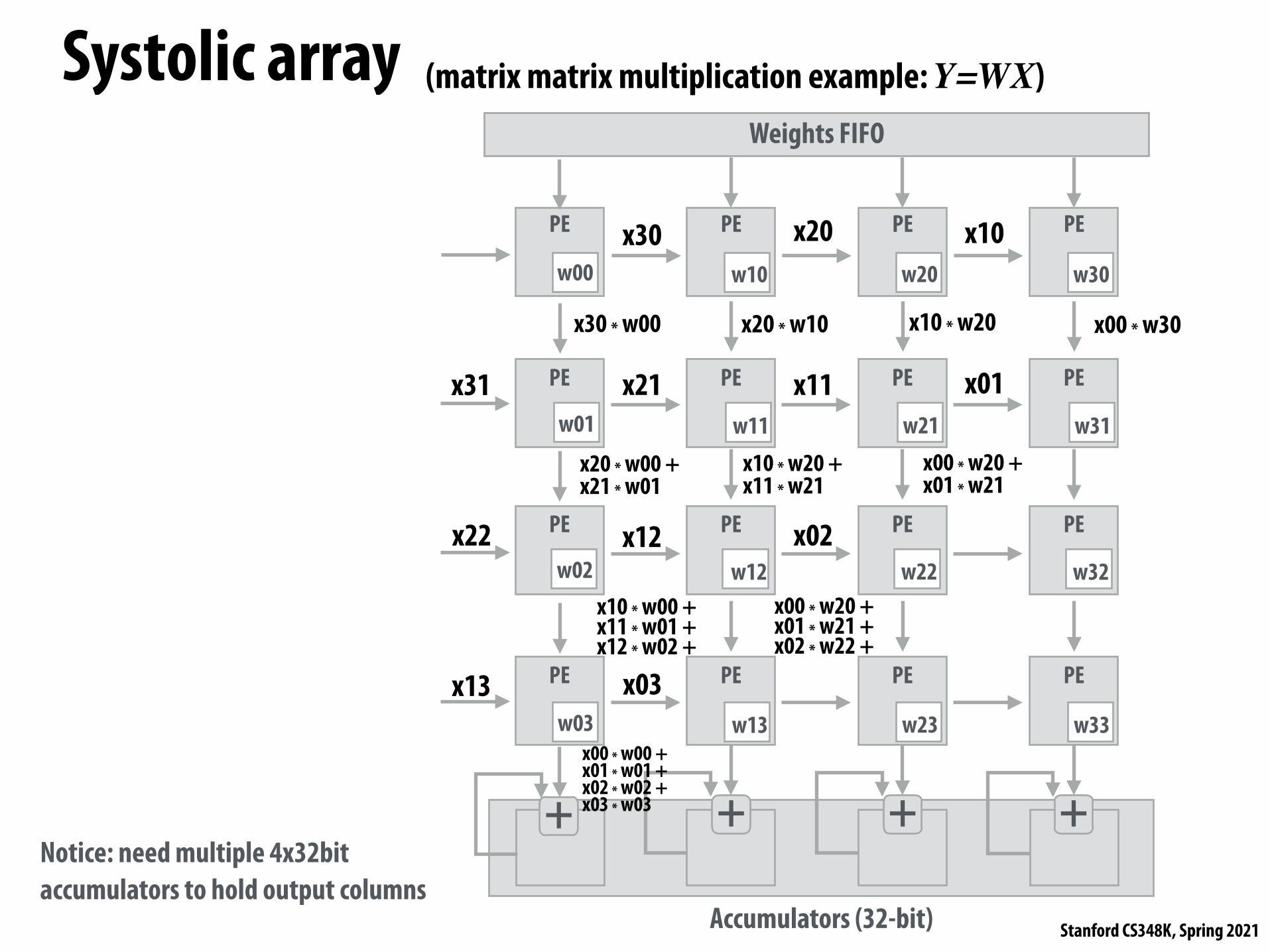
Systolic array (matrix matrix multiplication example: Y=WX)
PE PE PE PE
PE PE PE PE
PE PE PE PE
PE PE PE PE
Accumulators (32-bit)
+ + + +
Weights FIFO
w00
w01
w02
w03
w10
w11
w12
w13
w20
w21
w22
w23
w30
w31
w32
w33
x02
x00 * w20 + x01 * w21 + x02 * w22 +
x03
x01
x00 * w20 + x01 * w21
x00 * w30
x00 * w00 + x01 * w01 + x02 * w02 + x03 * w03
x12
x13
x11
x10
x10 * w00 + x11 * w01 + x12 * w02 +
x21
x22
x31
x20x30
x30 * w00 x20 * w10 x10 * w20
x10 * w20 + x11 * w21
x20 * w00 + x21 * w01
Notice: need multiple 4x32bit accumulators to hold output columns
Stanford CS348K, Spring 2021
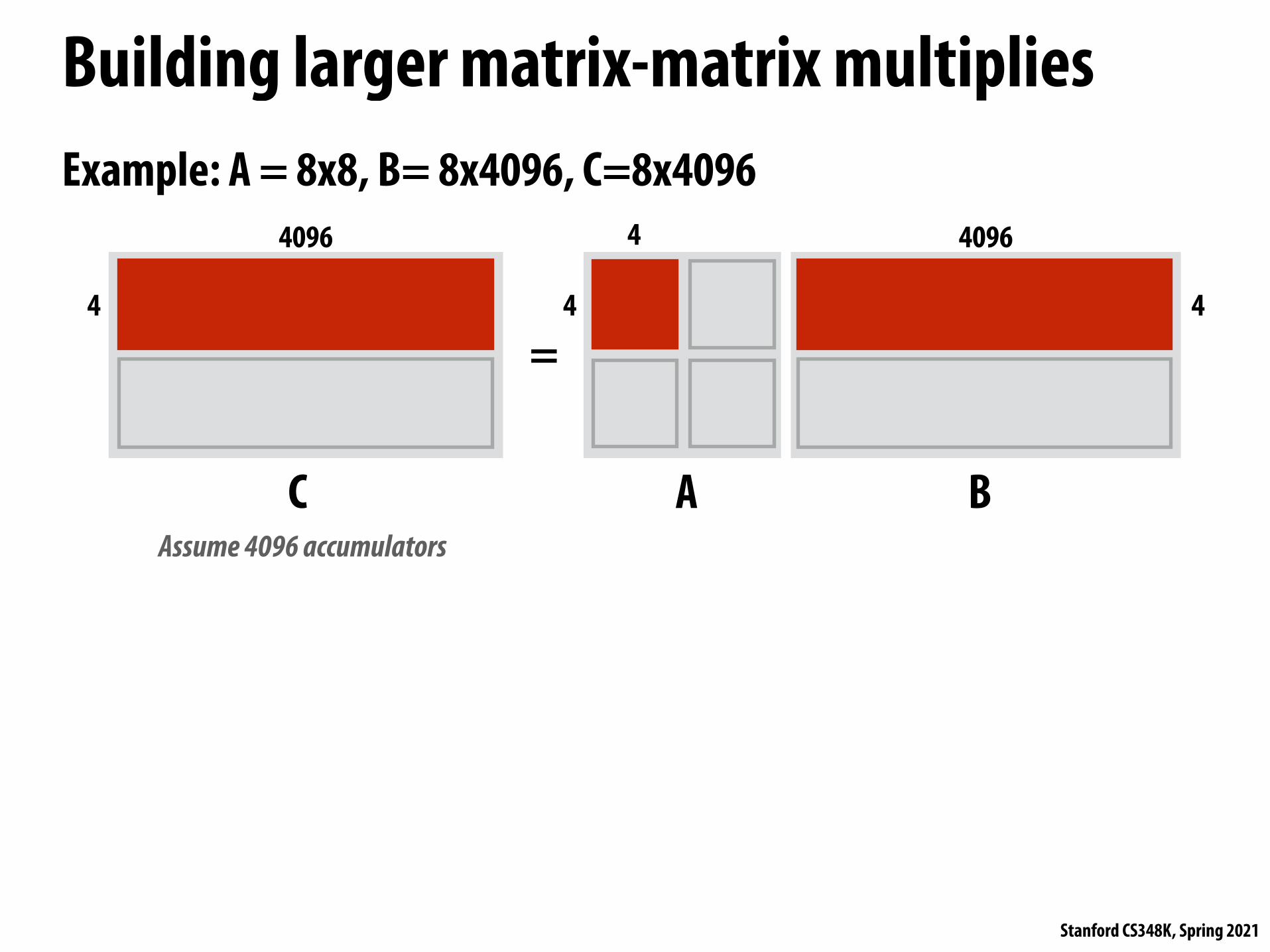
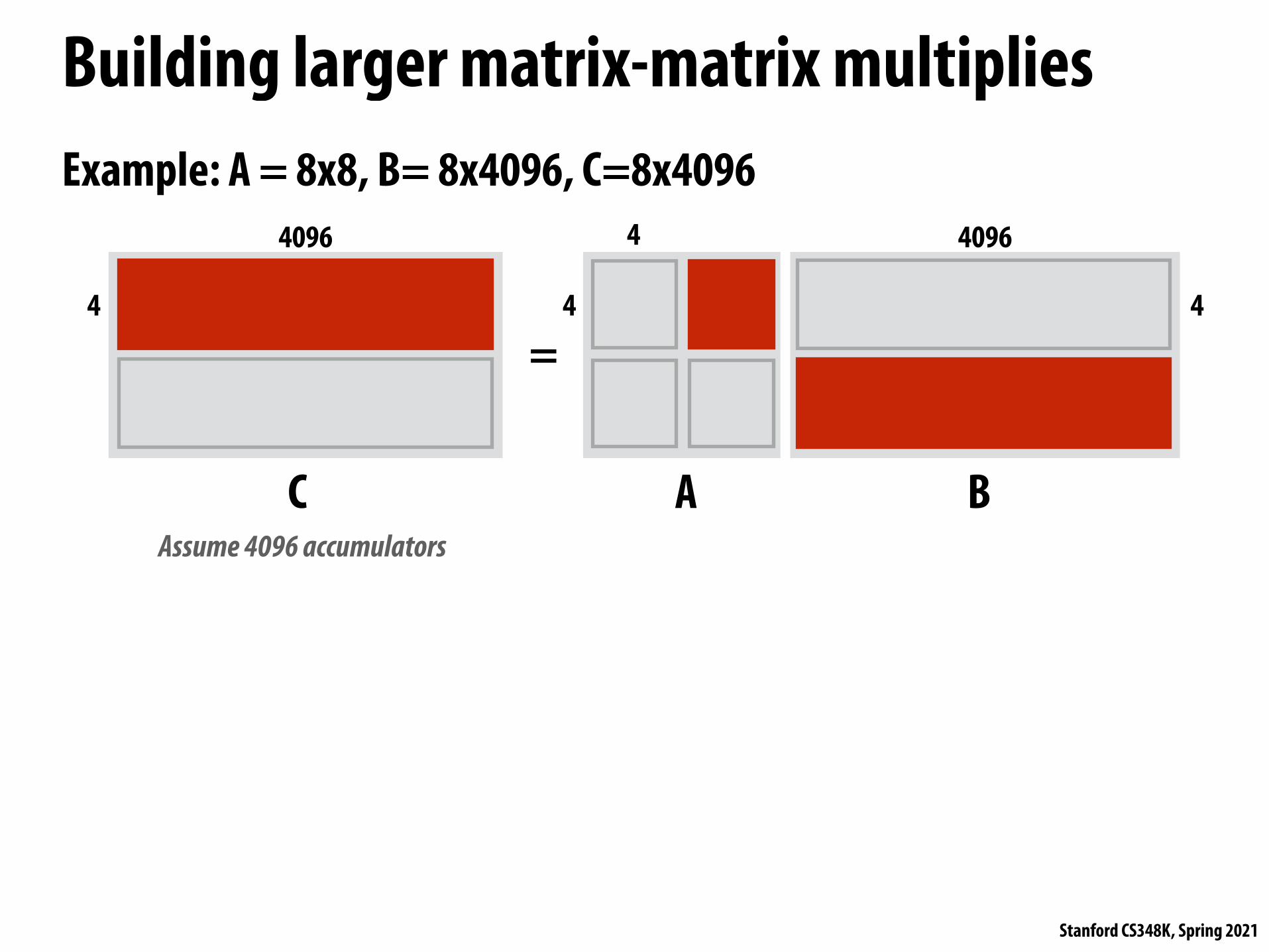
Building larger matrix-matrix multipliesExample: A = 8x8, B= 8x4096, C=8x4096
C
=
A B
4096
4 4
4 4096
4
Assume 4096 accumulators
Stanford CS348K, Spring 2021
Building larger matrix-matrix multipliesExample: A = 8x8, B= 8x4096, C=8x4096
C
=
A B
4096
4 4
4 4096
4
Assume 4096 accumulators

Stanford CS348K, Spring 2021
Building larger matrix-matrix multipliesExample: A = 8x8, B= 8x4096, C=8x4096
C
=
A B
4096
4 4
4 4096
4
Assume 4096 accumulators

Stanford CS348K, Spring 2021
Building larger matrix-matrix multipliesExample: A = 8x8, B= 8x4096, C=8x4096
C
=
A B
4096
4 4
4 4096
4
Assume 4096 accumulators

Stanford CS348K, Spring 2021
TPU Performance/Watt
Figure 8. Figures 5-7 combined into a single log-log graph. Stars are for the TPU, triangles are for the K80, and circles are for Haswell. All TPU stars are at or above the other 2 rooflines.
Figure 9. Relative performance/Watt (TDP) of GPU server (blue bar) and TPU server (red bar) to CPU server, and TPU server to GPU server (orange bar). TPU’ is an improved TPU (Sec. 7). The green bar shows its ratio to the CPU server and the lavender bar shows its relation to the GPU server. Total includes host server power, but incremental doesn’t. GM and WM are the geometric and weighted means.
9
GM = geometric mean over all apps WM = weighted mean over all apps
total = cost of host machine + CPU incremental = only cost of TPU
Figure credit: Jouppi et al. 2017

Stanford CS348K, Spring 2021
Alternative scheduling strategies
(a) Weight Stationary
(b) Output Stationary
(c) No Local Reuse
Fig. 8. Dataflows for DNNs.
PE 1
Row 1 Row 1
PE 2
Row 2 Row 2
PE 3
Row 3 Row 3
Row 1
= *
PE 4
Row 1 Row 2
PE 5
Row 2 Row 3
PE 6
Row 3 Row 4
Row 2
= *
PE 7
Row 1 Row 3
PE 8
Row 2 Row 4
PE 9
Row 3 Row 5
Row 3
= *
* * *
* * *
* * *
Fig. 9. Row Stationary Dataflow [34].
that area is allocated to the global buffer to increase itscapacity (Fig. 8(c)). The trade-off is that there will beincreased traffic on the spatial array and to the globalbuffer for all data types. Examples are found in [44–46].
• Row stationary (RS): In order to increase reuse ofall types of data (weights, pixels, partial sums), a rowstationary approach is proposed in [34]. A row of the filterconvolution remains stationary within a PE to exploit1-D convolutional reuse within the PE. Multiple 1-Drows are combined in the spatial array to exhaustivelyexploit all convolutional reuse (Fig. 9), which reducesaccesses to the global buffer. Multiple 1-D rows fromdifferent channels and filters are mapped to each PE toreduce partial sum data movement and exploit filter reuse,respectively. Finally, multiple passes across the spatialarray allow for additional image and filter reuse using theglobal buffer. This dataflow is demonstrated in [47].
The dataflows are compared on a spatial array with thesame number of PEs (256), area cost and DNN (AlexNet).Fig. 10 shows the energy consumption of each approach. Therow stationary approach is 1.4⇥ to 2.5⇥ more energy-efficient
0
0.5
1
1.5
2
Normalized Energy/MAC
WS OSA OSB OSC NLR RS
psums
weights
pixels
(a) Across types of data
Normalized Energy/MAC
ALU
RF
NoC
buffer
DRAM
0
0.5
1
1.5
2
WS OSA OSB OSC NLR RS
(b) Across levels of memory hierarchy
Fig. 10. Energy breakdown of dataflows [34].
than the other dataflows for the convolutional layers. Thisis due to the fact that the energy of all types of data isreduced. Furthermore, both the on-chip and off-chip energy isconsidered.
VI. OPPORTUNITIES IN JOINT ALGORITHM ANDHARDWARE DESIGN
There is on-going research on modifying the machinelearning algorithms to make them more hardware-friendly whilemaintaining accuracy; specifically, the focus is on reducingcomputation, data movement and storage requirements.
A. Reduce Precision
The default size for programmable platforms such asCPUs and GPUs is often 32 or 64 bits with floating-pointrepresentation. While this remains the case for training, duringinference, it is possible to use a fixed-point representation andsubstantially reduce the bitwidth for energy and area savings,and increase in throughput. Retraining is typically required tomaintain accuracy when pushing the weights and features tolower bitwidth.
In hand-crafted approaches, the bitwidth can be drasticallyreduced to below 16-bits without impacting the accuracy. Forinstance, in object detection using HOG, each 36-dimensionfeature vector only requires 9-bit per dimension, and eachweight of the SVM uses only 4-bits [48]; for object detectionusing deformable parts models (DPM) [49], only 11-bits arerequired per feature vector and only 5-bits are required perSVM weight [50].
Similarly for DNN inference, it is common to see acceleratorssupport 16-bit fixed point [45, 47]. There has been significant
TPU (v1) was “weight stationary”: weights kept in register at PE
each PE gets di$erent pixel partial sum pushed through array (array
has one output)
Figure credit: Sze et al. 2017
Psum = partial sum
“Output stationary”: each PE computes one output
push input pixel through array each PE gets di$erent weight
each PE accumulates locally into output
Takeaway: many DNN accelerators can be characterized by the data #ow of input
activations, weights, and outputs through the machine. (Just di$erent “schedules”!)

Stanford CS348K, Spring 2021
Input stationary design (dense 1D conv example)
out(0,i-1)
out(1,i-1)
out(0,i)
out(1,i) out(1,i+1)
out(0,i+1) out(0,i+2)
out(1,i+2)
in(i) in(i+1)
PE 0 PE 1
Accumulators (implement +=)
w(0,0)w(0,1)w(0,2)w(1,0)w(1,1)w(1,2)
Assume: 1D input/output 3-wide "lters 2 output channels (K=2)
6 5 4 3 2 1
123
46 5
WeightStream
Order
Processing elements
(implement multiply)
Stream of weights (2 1D "lters of size 3)

Stanford CS348K, Spring 2021
Scaling up (for training big models)Example: GPT-3 language model
(Amount of training — note this is log scale)
Very big models + More training = Better accuracy
Power law e$ect: exponentially more compute to take
constant step in accuracy

Stanford CS348K, Spring 2021
TPU v3 supercomputerTPU v3 board 4 TPU3 chips
One TPU v3 boardTPUs connected by
2D Torus interconnect
TPU supercomputer (1024 TPU v3 chips)

Stanford CS348K, Spring 2021
Additional examples of “AI chips”
Key ideas:
1. Huge numbers of compute units
2. Huge amounts of on-chip storage to maintain input weights and intermediate values

Stanford CS348K, Spring 2021
GraphCore MK2 GC200 IPU
900 MB on-chip storage
(59B transistors similar size to A100 GPU)
Access to o$-chip DDR4

Stanford CS348K, Spring 2021
Cerebras Wafer-Scale Engine (WSE)Tightly interconnected tile of chips (entire wafer) Many more transistors (1.2T) than largest single chips (Example: NVIDIA A100 GPU has 54B)
Compilation of DNN to platform involves “laying out” DNN layers in space on processing grid.

Stanford CS348K, Spring 2021
SambaNova recon"gurable data#ow unit Again, notice tight integration of storage and compute

Stanford CS348K, Spring 2021
Another example of spatial layout
Notice: inter-layer communication occurs through on-chip interconnect, not through o$-chip memory.

Stanford CS348K, Spring 2021
Exploiting sparsity

Stanford CS348K, Spring 2021
Architectural tricks for optimizing for sparsity▪ Consider operation: result += x*y ▪ If hardware determines contents of register x or register y is zero…
- Don’t "re ALU (save energy) - Don’t move data from register "le to ALU (save energy) - But ALU is idle (computation doesn’t run faster, optimization only saves energy)
SCNN ISCA ’17, June 24-28, 2017, Toronto, ON, Canada
0
0.2
0.4
0.6
0.8
1
0
0.2
0.4
0.6
0.8
1
conv1 conv2 conv3 conv4 conv5
Wor
k (#
of m
ultip
lies)
Dens
ity (I
A, W
)
Density (IA)Density (W)Work (# of multiplies)
(a) AlexNet
0
0.2
0.4
0.6
0.8
1
0
0.2
0.4
0.6
0.8
1
pool
_pro
j
1x1
3x3_
redu
ce 3x3
5x5_
redu
ce 5x5
pool
_pro
j
1x1
3x3_
redu
ce 3x3
5x5_
redu
ce 5x5
inception_3a inception_5b
Wor
k (#
of m
ultip
lies)
Dens
ity (I
A, W
)
Density (IA)Density (W)Work (# of multiplies)
(b) GoogLeNet
0
0.2
0.4
0.6
0.8
1
0
0.2
0.4
0.6
0.8
1
Wor
k (#
of m
ultip
lies)
Dens
ity (I
A, W
)
Density (IA)Density (W)Work (# of multiplies)
(c) VGGNet
Figure 1: Input activation and weight density and the reductionin the amount of work achievable by exploiting sparsity.
Sparsity in CNNs. Sparsity in a CNN layer is defined as thefraction of zeros in the layer’s weight and input activation matrices.The primary technique for creating weight sparsity is to prune thenetwork during training. Han, et al. developed a pruning algorithmthat operates in two phases [17]. First, any weight with an absolutevalue that is close to zero (e.g. below a defined threshold) is setto zero. This process has the effect of removing weights from thefilters, sometimes even forcing an output activation to always be zero.Second, the remaining network is retrained, to regain the accuracylost through naïve pruning. The result is a smaller network withaccuracy extremely close to the original network. The process canbe iteratively repeated to reduce network size while maintainingaccuracy.
Activation sparsity occurs dynamically during inference and ishighly dependent on the data being processed. Specifically, the rec-tified linear unit (ReLU) function that is commonly used as thenon-linear operator in CNNs forces all negatively valued activations
Table 2: Qualitative comparison of sparse CNN accelerators.
GateMACC
SkipMACC
SkipInner spatial
dataflowbuffer/
Architecture DRAMaccess
Eyeriss [7] A – A Row StationaryCnvlutin [1] A A A Vector Scalar + ReductionCambricon-X [34] W W W Dot ProductSCNN A+W A+W A+W Cartesian Product
to be clamped to zero. After completing computation of a convolu-tional layer, a ReLU function is applied point-wise to each elementin the output activation matrices before the data is passed to the nextlayer.
To measure the weight and activation sparsity, we used the Caffeframework [4] to prune and train the three networks listed in Ta-ble 1, using the pruning algorithm of [17]. We then instrumentedthe Caffe framework to inspect the activations between the convo-lutional layers. Figure 1 shows the weight and activation density(fraction of non-zeros or complement of sparsity) of the layers of thenetworks, referenced to the left-hand y-axes. As GoogLeNet has 54convolutional layers, we only show a subset of representative layers.The data shows that weight density varies across both layers andnetworks, reaching a minimum of 30% for some of the GoogLeNetlayers. Activation density also varies, with density typically beinghigher in early layers. Activation density can be as low as 30% aswell. The triangles show the ideal number of multiplies that couldbe achieved if all multiplies with a zero operand are eliminated. Thisis calculated by by taking the product of the weight and activationdensities on a per-layer basis.
Exploiting sparsity. Since multiplication by zero just results ina zero, it should require no work. Thus, typical layers can reducework by a factor of four, and can reach as high as a factor of ten. Inaddition, those zero products will contribute nothing to the partialsum it is part of, so the addition is unnecessary as well. Furthermore,data with many zeros can be represented in a compressed form.Together these characteristics provide a number of opportunities foroptimization:
• Compressing data: Encoding the sparse weights and/oractivations provides an architecture an opportunity to re-duce the amount of data that must be moved throughout thememory hierarchy. It also reduces the data footprint, whichallows larger matrices to be held in a storage structure of agiven size.
• Eliminating computation: For multiplications that have azero weight and/or activation operand, the operation canbe data gated, or the operands might never be sent to themultiplier. This optimization can save energy consumptionor both time and energy consumption, respectively.
Table 2 describes how several recent CNN accelerator architectureexploit sparsity. Eyeriss [7] exploits sparsity in activations by storingthem in compressed form in DRAM and by gating computation cy-cles for zero-valued activations to save energy. Cnvlutin [1] is moreaggressive—the architecture moves and stages sparse activationsin compressed form and skips computation cycles for zero-valuedactivations to improve both performance and energy efficiency. Both

Stanford CS348K, Spring 2021
Recall: model compression- Step 1: sparsify weights by truncating weights with small values to zero - Step 2: compress surviving non-zeros
- Cluster weights via k-means clustering - Compress weights by only storing index of assigned cluster (lg(k) bits)
Published as a conference paper at ICLR 2016
Figure 2: Representing the matrix sparsity with relative index. Padding filler zero to prevent overflow.
2.09 -0.98 1.48 0.09
0.05 -0.14 -1.08 2.12
-0.91 1.92 0 -1.03
1.87 0 1.53 1.49
cluster
weights (32 bit float) centroids
gradient
3 0 2 1
1 1 0 3
0 3 1 0
3 1 2 2
cluster index (2 bit uint)
2.00
1.50
0.00
-1.00
1:
0:
2:
3:
Figure 3: Weight sharing by scalar quantization (top) and centroids fine-tuning (bottom).
We store the sparse structure that results from pruning using compressed sparse row (CSR) orcompressed sparse column (CSC) format, which requires 2a+n+1 numbers, where a is the numberof non-zero elements and n is the number of rows or columns.
To compress further, we store the index difference instead of the absolute position, and encode thisdifference in 8 bits for conv layer and 5 bits for fc layer. When we need an index difference largerthan the bound, we the zero padding solution shown in Figure 2: in case when the difference exceeds8, the largest 3-bit (as an example) unsigned number, we add a filler zero.
3 TRAINED QUANTIZATION AND WEIGHT SHARING
Network quantization and weight sharing further compresses the pruned network by reducing thenumber of bits required to represent each weight. We limit the number of effective weights we need tostore by having multiple connections share the same weight, and then fine-tune those shared weights.
Weight sharing is illustrated in Figure 3. Suppose we have a layer that has 4 input neurons and 4output neurons, the weight is a 4⇥ 4 matrix. On the top left is the 4⇥ 4 weight matrix, and on thebottom left is the 4⇥ 4 gradient matrix. The weights are quantized to 4 bins (denoted with 4 colors),all the weights in the same bin share the same value, thus for each weight, we then need to store onlya small index into a table of shared weights. During update, all the gradients are grouped by the colorand summed together, multiplied by the learning rate and subtracted from the shared centroids fromlast iteration. For pruned AlexNet, we are able to quantize to 8-bits (256 shared weights) for eachCONV layers, and 5-bits (32 shared weights) for each FC layer without any loss of accuracy.
To calculate the compression rate, given k clusters, we only need log2(k) bits to encode the index. Ingeneral, for a network with n connections and each connection is represented with b bits, constrainingthe connections to have only k shared weights will result in a compression rate of:
r =nb
nlog2(k) + kb(1)
For example, Figure 3 shows the weights of a single layer neural network with four input units andfour output units. There are 4⇥4 = 16 weights originally but there are only 4 shared weights: similarweights are grouped together to share the same value. Originally we need to store 16 weights each
3
[Han et al. ]
[Figure credit: Han ICLR16]

Stanford CS348K, Spring 2021
Sparse, weight-sharing fully-connected layer
to dense form before operation [11]. Neither is able toexploit weight sharing. This motivates building a specialengine that can operate on a compressed network.
III. DNN COMPRESSION AND PARALLELIZATION
A. Computation
A FC layer of a DNN performs the computation
b = f(Wa+ v) (1)
Where a is the input activation vector, b is the outputactivation vector, v is the bias, W is the weight matrix, andf is the non-linear function, typically the Rectified LinearUnit(ReLU) [22] in CNN and some RNN. Sometimes v
will be combined with W by appending an additional oneto vector a, therefore we neglect the bias in the followingparagraphs.
For a typical FC layer like FC7 of VGG-16 or AlexNet,the activation vectors are 4K long, and the weight matrix is4K ⇥ 4K (16M weights). Weights are represented as single-precision floating-point numbers so such a layer requires64MB of storage. The output activations of Equation (1) arecomputed element-wise as:
bi = ReLU
0
@n�1X
j=0
Wijaj
1
A (2)
Deep Compression [23] describes a method to compressDNNs without loss of accuracy through a combination ofpruning and weight sharing. Pruning makes matrix W sparsewith density D ranging from 4% to 25% for our benchmarklayers. Weight sharing replaces each weight Wij with a four-bit index Iij into a shared table S of 16 possible weightvalues.
With deep compression, the per-activation computation ofEquation (2) becomes
bi = ReLU
0
@X
j2Xi\Y
S[Iij ]aj
1
A (3)
Where Xi is the set of columns j for which Wij 6= 0, Yis the set of indices j for which aj 6= 0, Iij is the indexto the shared weight that replaces Wij , and S is the tableof shared weights. Here Xi represents the static sparsity ofW and Y represents the dynamic sparsity of a. The set Xi
is fixed for a given model. The set Y varies from input toinput.
Accelerating Equation (3) is needed to accelerate a com-pressed DNN. We perform the indexing S[Iij ] and themultiply-add only for those columns for which both Wij
and aj are non-zero, so that both the sparsity of the matrixand the vector are exploited. This results in a dynamically ir-regular computation. Performing the indexing itself involves
~a�
0 0 a2 0 a4 a5 0 a7
�
⇥ ~b
PE0
PE1
PE2
PE3
0
BBBBBBBBBBBBBBBBBBBBBBBBBBBBBBBB@
w0,0 0 w0,2 0 w0,4 w0,5 w0,6 0
0 w1,1 0 w1,3 0 0 w1,6 0
0 0 w2,2 0 w2,4 0 0 w2,7
0 w3,1 0 0 0 w0,5 0 0
0 w4,1 0 0 w4,4 0 0 0
0 0 0 w5,4 0 0 0 w5,7
0 0 0 0 w6,4 0 w6,6 0
w7,0 0 0 w7,4 0 0 w7,7 0
w8,0 0 0 0 0 0 0 w8,7
w9,0 0 0 0 0 0 w9,6 w9,7
0 0 0 0 w10,4 0 0 0
0 0 w11,2 0 0 0 0 w11,7
w12,0 0 w12,2 0 0 w12,5 0 w12,7
w13,0w13,2 0 0 0 0 w13,6 0
0 0 w14,2w14,3w14,4w14,5 0 0
0 0 w15,2w15,3 0 w15,5 0 0
1
CCCCCCCCCCCCCCCCCCCCCCCCCCCCCCCCA
=
0
BBBBBBBBBBBBBBBBBBBBBBBBBBBBBBBB@
b0
b1
�b2
b3
�b4
b5
b6
�b7
�b8
�b9
b10
�b11
�b12
b13
b14
�b15
1
CCCCCCCCCCCCCCCCCCCCCCCCCCCCCCCCA
ReLU)
0
BBBBBBBBBBBBBBBBBBBBBBBBBBBBBBBB@
b0
b1
0
b3
0
b5
b6
0
0
0
b10
0
0
b13
b14
0
1
CCCCCCCCCCCCCCCCCCCCCCCCCCCCCCCCA
1
Figure 2. Matrix W and vectors a and b are interleaved over 4 PEs.Elements of the same color are stored in the same PE.
VirtualWeight
W0,0 W8,0 W12,0 W4,1 W0,2 W12,2 W0,4 W4,4 W0,5 W12,5 W0,6 W8,7 W12,7
Relative RowIndex 0 1 0 1 0 2 0 0 0 2 0 2 0
ColumnPointer 0 3 4 6 6 8 10 11 13
Figure 3. Memory layout for the relative indexed, indirect weighted andinterleaved CSC format, corresponding to PE0 in Figure 2.
bit manipulations to extract four-bit Iij and an extra load(which is almost assured a cache hit).
B. Representation
To exploit the sparsity of activations we store our encodedsparse weight matrix W in a variation of compressed sparsecolumn (CSC) format [24].
For each column Wj of matrix W we store a vector v
that contains the non-zero weights, and a second, equal-length vector z that encodes the number of zeros beforethe corresponding entry in v. Each entry of v and z isrepresented by a four-bit value. If more than 15 zeros appearbefore a non-zero entry we add a zero in vector v. Forexample, we encode the following column
[0, 0, 1, 2, 0, 0, 0, 0, 0, 0, 0, 0, 0, 0, 0, 0, 0, 0, 0,0, 0, 0, 3]
as v = [1, 2,0, 3], z = [2, 0,15, 2]. v and z of all columnsare stored in one large pair of arrays with a pointer vector ppointing to the beginning of the vector for each column. Afinal entry in p points one beyond the last vector element sothat the number of non-zeros in column j (including paddedzeros) is given by pj+1 � pj .
Storing the sparse matrix by columns in CSC formatmakes it easy to exploit activation sparsity. We simplymultiply each non-zero activation by all of the non-zeroelements in its corresponding column.
Fully-connected layer: Matrix-vector multiplication of activation vector a against weight matrix W
Sparse, weight-sharing representation: Iij = index for weight Wij
S[] = table of shared weight values Xi = list of non-zero indices in row i Y = list of non-zero indices in vector a
Note: activations can be sparse due to ReLU

Stanford CS348K, Spring 2021
Sparse-matrix, vector multiplicationRepresent weight matrix in compressed sparse column (CSC) format to exploit sparsity in activation vector:
for each nonzero a_j in a: for each nonzero M_ij in column M_j: b_i += M_ij * a_j
int16* a_values; // dense PTR* M_j_start; // column j int4* M_j_values; int4* M_j_indices; int16* lookup; // lookup table for // cluster values (from // deep compression paper)
More detailed version (assumes CSC matrix): for j=0 to length(a): if (a[j] == 0) continue; // scan to next nonzero col_values = M_j_values[M_j_start[j]]; // j-th col col_indices = M_j_indices[M_j_start[j]]; // row idx in col col_nonzeros = M_j_start[j+1] - M_j_start[j]; for i=0, i_count=0 to col_nonzeros: i += col_indices[i_count]; b[i] += lookup[col_values[i_count]] * a_values[j];
* Recall from deep compression paper: there is a unique lookup table for each chunk of matrix values

Stanford CS348K, Spring 2021
Parallelization of sparse-matrix-vector productStride rows of matrix across processing elements Output activations strided across processing elements
to dense form before operation [11]. Neither is able toexploit weight sharing. This motivates building a specialengine that can operate on a compressed network.
III. DNN COMPRESSION AND PARALLELIZATION
A. Computation
A FC layer of a DNN performs the computation
b = f(Wa+ v) (1)
Where a is the input activation vector, b is the outputactivation vector, v is the bias, W is the weight matrix, andf is the non-linear function, typically the Rectified LinearUnit(ReLU) [22] in CNN and some RNN. Sometimes v
will be combined with W by appending an additional oneto vector a, therefore we neglect the bias in the followingparagraphs.
For a typical FC layer like FC7 of VGG-16 or AlexNet,the activation vectors are 4K long, and the weight matrix is4K ⇥ 4K (16M weights). Weights are represented as single-precision floating-point numbers so such a layer requires64MB of storage. The output activations of Equation (1) arecomputed element-wise as:
bi = ReLU
0
@n�1X
j=0
Wijaj
1
A (2)
Deep Compression [23] describes a method to compressDNNs without loss of accuracy through a combination ofpruning and weight sharing. Pruning makes matrix W sparsewith density D ranging from 4% to 25% for our benchmarklayers. Weight sharing replaces each weight Wij with a four-bit index Iij into a shared table S of 16 possible weightvalues.
With deep compression, the per-activation computation ofEquation (2) becomes
bi = ReLU
0
@X
j2Xi\Y
S[Iij ]aj
1
A (3)
Where Xi is the set of columns j for which Wij 6= 0, Yis the set of indices j for which aj 6= 0, Iij is the indexto the shared weight that replaces Wij , and S is the tableof shared weights. Here Xi represents the static sparsity ofW and Y represents the dynamic sparsity of a. The set Xi
is fixed for a given model. The set Y varies from input toinput.
Accelerating Equation (3) is needed to accelerate a com-pressed DNN. We perform the indexing S[Iij ] and themultiply-add only for those columns for which both Wij
and aj are non-zero, so that both the sparsity of the matrixand the vector are exploited. This results in a dynamically ir-regular computation. Performing the indexing itself involves
~a�
0 0 a2 0 a4 a5 0 a7
�
⇥ ~b
PE0
PE1
PE2
PE3
0
BBBBBBBBBBBBBBBBBBBBBBBBBBBBBBBB@
w0,0 0 w0,2 0 w0,4 w0,5 w0,6 0
0 w1,1 0 w1,3 0 0 w1,6 0
0 0 w2,2 0 w2,4 0 0 w2,7
0 w3,1 0 0 0 w0,5 0 0
0 w4,1 0 0 w4,4 0 0 0
0 0 0 w5,4 0 0 0 w5,7
0 0 0 0 w6,4 0 w6,6 0
w7,0 0 0 w7,4 0 0 w7,7 0
w8,0 0 0 0 0 0 0 w8,7
w9,0 0 0 0 0 0 w9,6 w9,7
0 0 0 0 w10,4 0 0 0
0 0 w11,2 0 0 0 0 w11,7
w12,0 0 w12,2 0 0 w12,5 0 w12,7
w13,0w13,2 0 0 0 0 w13,6 0
0 0 w14,2w14,3w14,4w14,5 0 0
0 0 w15,2w15,3 0 w15,5 0 0
1
CCCCCCCCCCCCCCCCCCCCCCCCCCCCCCCCA
=
0
BBBBBBBBBBBBBBBBBBBBBBBBBBBBBBBB@
b0
b1
�b2
b3
�b4
b5
b6
�b7
�b8
�b9
b10
�b11
�b12
b13
b14
�b15
1
CCCCCCCCCCCCCCCCCCCCCCCCCCCCCCCCA
ReLU)
0
BBBBBBBBBBBBBBBBBBBBBBBBBBBBBBBB@
b0
b1
0
b3
0
b5
b6
0
0
0
b10
0
0
b13
b14
0
1
CCCCCCCCCCCCCCCCCCCCCCCCCCCCCCCCA
1
Figure 2. Matrix W and vectors a and b are interleaved over 4 PEs.Elements of the same color are stored in the same PE.
VirtualWeight
W0,0 W8,0 W12,0 W4,1 W0,2 W12,2 W0,4 W4,4 W0,5 W12,5 W0,6 W8,7 W12,7
Relative RowIndex 0 1 0 1 0 2 0 0 0 2 0 2 0
ColumnPointer 0 3 4 6 6 8 10 11 13
Figure 3. Memory layout for the relative indexed, indirect weighted andinterleaved CSC format, corresponding to PE0 in Figure 2.
bit manipulations to extract four-bit Iij and an extra load(which is almost assured a cache hit).
B. Representation
To exploit the sparsity of activations we store our encodedsparse weight matrix W in a variation of compressed sparsecolumn (CSC) format [24].
For each column Wj of matrix W we store a vector v
that contains the non-zero weights, and a second, equal-length vector z that encodes the number of zeros beforethe corresponding entry in v. Each entry of v and z isrepresented by a four-bit value. If more than 15 zeros appearbefore a non-zero entry we add a zero in vector v. Forexample, we encode the following column
[0, 0, 1, 2, 0, 0, 0, 0, 0, 0, 0, 0, 0, 0, 0, 0, 0, 0, 0,0, 0, 0, 3]
as v = [1, 2,0, 3], z = [2, 0,15, 2]. v and z of all columnsare stored in one large pair of arrays with a pointer vector ppointing to the beginning of the vector for each column. Afinal entry in p points one beyond the last vector element sothat the number of non-zeros in column j (including paddedzeros) is given by pj+1 � pj .
Storing the sparse matrix by columns in CSC formatmakes it easy to exploit activation sparsity. We simplymultiply each non-zero activation by all of the non-zeroelements in its corresponding column.
Weights stored local to PEs. Must broadcast non-zero a_j’s to all PEs Accumulation of each output b_i is local to PE
0 0 a2 0 a4 a5 0 a7

Stanford CS348K, Spring 2021
E!cient Inference Engine (EIE) for quantized sparse/matrix vector product
Pointer Read Act R/W
Act Queue
Sparse Matrix Access
Sparse Matrix SRAM
Arithmetic Unit
Regs
Col Start/End
Addr
Act Index
Weight Decoder
Address Accum
Dest Act
Regs
Act SRAM
Act Value
Encoded Weight
Relative Index
Src Act
Regs Absolute Address
Bypass
Leading NZero Detect
Even Ptr SRAM Bank
Odd Ptr SRAM Bank ReLU
(b) Figure 4. (a) The architecture of Leading Non-zero Detection Node. (b) The architecture of Processing Element.
C. Parallelizing Compressed DNN
We distribute the matrix and parallelize our matrix-vectorcomputation by interleaving the rows of the matrix W overmultiple processing elements (PEs). With N PEs, PEk holdsall rows Wi, output activations bi, and input activations ai
for which i (mod N) = k. The portion of column Wj inPEk is stored in the CSC format described in Section III-Bbut with the zero counts referring only to zeros in the subsetof the column in this PE. Each PE has its own v, x, and p
arrays that encode its fraction of the sparse matrix.Figure 2 shows an example multiplying an input activation
vector a (of length 8) by a 16⇥8 weight matrix W yieldingan output activation vector b (of length 16) on N = 4 PEs.The elements of a, b, and W are color coded with their PEassignments. Each PE owns 4 rows of W , 2 elements of a,and 4 elements of b.
We perform the sparse matrix ⇥ sparse vector operationby scanning vector a to find its next non-zero value aj
and broadcasting aj along with its index j to all PEs.Each PE then multiplies aj by the non-zero elements inits portion of column Wj — accumulating the partial sumsin accumulators for each element of the output activationvector b. In the CSC representation these non-zeros weightsare stored contiguously so each PE simply walks through itsv array from location pj to pj+1 � 1 to load the weights.To address the output accumulators, the row number i
corresponding to each weight Wij is generated by keepinga running sum of the entries of the x array.
In the example of Figure 2, the first non-zero is a2 onPE2. The value a2 and its column index 2 is broadcastto all PEs. Each PE then multiplies a2 by every non-zero in its portion of column 2. PE0 multiplies a2 byW0,2 and W12,2; PE1 has all zeros in column 2 and soperforms no multiplications; PE2 multiplies a2 by W2,2
and W14,2, and so on. The result of each product is summedinto the corresponding row accumulator. For example PE0
computes b0 = b0 + W0,2a2 and b12 = b12 + W12,2a2.The accumulators are initialized to zero before each layercomputation.
The interleaved CSC representation facilitates exploitationof both the dynamic sparsity of activation vector a andthe static sparsity of the weight matrix W . We exploit
activation sparsity by broadcasting only non-zero elementsof input activation a. Columns corresponding to zeros in a
are completely skipped. The interleaved CSC representationallows each PE to quickly find the non-zeros in each columnto be multiplied by aj . This organization also keeps all of thecomputation except for the broadcast of the input activationslocal to a PE. The interleaved CSC representation of matrixin Figure 2 is shown in Figure 3.
This process may suffer load imbalance because each PEmay have a different number of non-zeros in a particularcolumn. We will see in Section IV how this load imbalancecan be reduced by queuing.
IV. HARDWARE IMPLEMENTATION
Figure 4 shows the architecture of EIE. A Central ControlUnit (CCU) controls an array of PEs that each computes oneslice of the compressed network. The CCU also receivesnon-zero input activations from a distributed leading non-zero detection network and broadcasts these to the PEs.
Almost all computation in EIE is local to the PEs exceptfor the collection of non-zero input activations that arebroadcast to all PEs. However, the timing of the activationcollection and broadcast is non-critical as most PEs takemany cycles to consume each input activation.
Activation Queue and Load Balancing. Non-zero ele-ments of the input activation vector aj and their correspond-ing index j are broadcast by the CCU to an activation queuein each PE. The broadcast is disabled if any PE has a fullqueue. At any point in time each PE processes the activationat the head of its queue.
The activation queue allows each PE to build up a backlogof work to even out load imbalance that may arise becausethe number of non zeros in a given column j may varyfrom PE to PE. In Section VI we measure the sensitivity ofperformance to the depth of the activation queue.
Pointer Read Unit. The index j of the entry at the headof the activation queue is used to look up the start and endpointers pj and pj+1 for the v and x arrays for column j.To allow both pointers to be read in one cycle using single-ported SRAM arrays, we store pointers in two SRAM banksand use the LSB of the address to select between banks. pjand pj+1 will always be in different banks. EIE pointers are16-bits in length.
Tuple representing non-zero activation (aj, j) arrives and is enqueuedCustom hardware for decoding compressed-sparse representation

Stanford CS348K, Spring 2021
EIE e!ciency
1x 1x 1x 1x 1x 1x 1x 1x 1x 1x2x
5x1x
9x 10x
1x2x 3x 2x 3x
14x25x
14x 24x 22x10x 9x 15x 9x 15x
56x 94x
21x
210x 135x
16x34x 33x 25x
48x
0.6x1.1x
0.5x1.0x 1.0x
0.3x 0.5x 0.5x 0.5x 0.6x
3x5x
1x
8x 9x
1x3x 2x 1x
3x
248x507x
115x
1018x 618x
92x 63x 98x 60x189x
0.1x
1x
10x
100x
1000x
Alex-6 Alex-7 Alex-8 VGG-6 VGG-7 VGG-8 NT-We NT-Wd NT-LSTM Geo Mean
Speedup
CPU Dense (Baseline) CPU Compressed GPU Dense GPU Compressed mGPU Dense mGPU Compressed EIE
Figure 6. Speedups of GPU, mobile GPU and EIE compared with CPU running uncompressed DNN model. There is no batching in all cases.
1x 1x 1x 1x 1x 1x 1x 1x 1x 1x5x
9x3x
17x 20x
2x6x 6x 4x 6x7x 12x 7x 10x 10x
5x 6x 6x 5x 7x26x 37x
10x
78x 61x
8x25x 14x 15x 23x
10x 15x7x 13x 14x
5x 8x 7x 7x 9x
37x 59x18x
101x 102x
14x39x 25x 20x 36x
34,522x 61,533x14,826x
119,797x 76,784x
11,828x 9,485x 10,904x 8,053x24,207x
1x
10x
100x
1000x
10000x
100000x
Alex-6 Alex-7 Alex-8 VGG-6 VGG-7 VGG-8 NT-We NT-Wd NT-LSTM Geo MeanEner
gy E
ffici
ency
CPU Dense (Baseline) CPU Compressed GPU Dense GPU Compressed mGPU Dense mGPU Compressed EIE
Figure 7. Energy efficiency of GPU, mobile GPU and EIE compared with CPU running uncompressed DNN model. There is no batching in all cases.
energy numbers. We annotated the toggle rate from the RTLsimulation to the gate-level netlist, which was dumped toswitching activity interchange format (SAIF), and estimatedthe power using Prime-Time PX.
Comparison Baseline. We compare EIE with three dif-ferent off-the-shelf computing units: CPU, GPU and mobileGPU.
1) CPU. We use Intel Core i-7 5930k CPU, a Haswell-Eclass processor, that has been used in NVIDIA Digits DeepLearning Dev Box as a CPU baseline. To run the benchmarkon CPU, we used MKL CBLAS GEMV to implement theoriginal dense model and MKL SPBLAS CSRMV for thecompressed sparse model. CPU socket and DRAM powerare as reported by the pcm-power utility provided by Intel.
2) GPU. We use NVIDIA GeForce GTX Titan X GPU,a state-of-the-art GPU for deep learning as our baselineusing nvidia-smi utility to report the power. To runthe benchmark, we used cuBLAS GEMV to implementthe original dense layer. For the compressed sparse layer,we stored the sparse matrix in in CSR format, and usedcuSPARSE CSRMV kernel, which is optimized for sparsematrix-vector multiplication on GPUs.
3) Mobile GPU. We use NVIDIA Tegra K1 that has192 CUDA cores as our mobile GPU baseline. We usedcuBLAS GEMV for the original dense model and cuS-PARSE CSRMV for the compressed sparse model. Tegra K1doesn’t have software interface to report power consumption,so we measured the total power consumption with a power-meter, then assumed 15% AC to DC conversion loss, 85%regulator efficiency and 15% power consumed by peripheralcomponents [26], [27] to report the AP+DRAM power forTegra K1.
Benchmarks. We compare the performance on two setsof models: uncompressed DNN model and the compressedDNN model. The uncompressed DNN model is obtainedfrom Caffe model zoo [28] and NeuralTalk model zoo [7];The compressed DNN model is produced as described
Table IIIBENCHMARK FROM STATE-OF-THE-ART DNN MODELS
Layer Size Weight% Act% FLOP% Description
Alex-6 9216, 9% 35.1% 3% Compressed4096AlexNet [1] forAlex-7 4096, 9% 35.3% 3% large scale image4096classificationAlex-8 4096, 25% 37.5% 10%1000
VGG-6 25088, 4% 18.3% 1% Compressed4096 VGG-16 [3] forVGG-7 4096, 4% 37.5% 2% large scale image4096 classification andVGG-8 4096, 23% 41.1% 9% object detection1000
NT-We 4096, 10% 100% 10% Compressed600 NeuralTalk [7]
NT-Wd 600, 11% 100% 11% with RNN and8791 LSTM for
NTLSTM 1201, 10% 100% 11% automatic2400 image captioning
in [16], [23]. The benchmark networks have 9 layers in totalobtained from AlexNet, VGGNet, and NeuralTalk. We usethe Image-Net dataset [29] and the Caffe [28] deep learningframework as golden model to verify the correctness of thehardware design.
VI. EXPERIMENTAL RESULTS
Figure 5 shows the layout (after place-and-route) ofan EIE processing element. The power/area breakdown isshown in Table II. We brought the critical path delay downto 1.15ns by introducing 4 pipeline stages to update oneactivation: codebook lookup and address accumulation (inparallel), output activation read and input activation multiply(in parallel), shift and add, and output activation write. Ac-tivation read and write access a local register and activationbypassing is employed to avoid a pipeline hazard. Using64 PEs running at 800MHz yields a performance of 102GOP/s. Considering 10⇥ weight sparsity and 3⇥ activationsparsity, this requires a dense DNN accelerator 3TOP/s tohave equivalent application throughput.
CPU: Core i7 5930k (6 cores) GPU: GTX Titan X mGPU: Tegra K1
Sources of energy savings: - Compression allows all weights to be stored in SRAM (reduce DRAM loads) - Low-precision 16-bit "xed-point math (5x more e!cient than 32-bit "xed math) - Skip math on input activations that are zero (65% less math)
Warning: these are not end-to-end numbers: just fully connected layers!

Stanford CS348K, Spring 2021
Reminder: input stationary design (dense 1D)
out(0,i-1)
out(1,i-1)
out(0,i)
out(1,i) out(1,i+1)
out(0,i+1) out(0,i+2)
out(1,i+2)
in(i) in(i+1)
PE 0 PE 1
Accumulators (implement +=)
Processing elements
(implement multiply)
w(0,0)w(0,1)w(0,2)w(1,0)w(1,1)w(1,2)
Assume: 1D input/output 3-wide "lters 2 output channels (K=2) Stream of weights
(2 1D "lters of size 3)
6 5 4 3 2 1
123
46 5
WeightStream
Order

Stanford CS348K, Spring 2021
Input stationary design (sparse example)
in(i) in(j)
PE 0 PE 1
Accumulators (implement +=)
Processing elements
w(0,0)w(0,2)w(1,1)w(1,2)
Assume: 1D input/output 3-wide SPARSE "lters 2 output channels (K=2) Stream of sparse weights
(2 "lters, each with 2 non-zeros)4 3 2 1
WeightStream
Order
12 12
34
3
4
Note: accumulate is now a scatterDense output bu$er
out(0,i-1)
out(1,i-1)
out(0,i+1) out(0,j-1)
out(1,j-1)
out(0,j+1)
out(1,i) out(1,j)

Stanford CS348K, Spring 2021
SCNN: accelerating sparse conv layers
SCNN ISCA ’17, June 24-28, 2017, Toronto, ON, Canada
1
F
F�I
FxI multiplier array
Coordinate Computation
F
I F�I
A accumulator buffers
Neighbors
PPU Halos ReLU
Compress
IARAM (sparse)
IARAM indices
OARAM (sparse)
OARAM indices
Buffer bank
…
Buffer bank
…
…
…
I
F�I x
A
arbi
trat
ed X
BAR
Weight FIFO (sparse)
indices
DRAM
DRAM
Figure 6: SCNN PE employing the PT-IS-CP-sparse dataflow.
connected layers are similar in nature to the convolution layers, theydo require much larger weight matrices. However, recent work hasdemonstrated effective DNNs without fully connected layers [24].Section 4.3 describes further how FC layers can be processed bySCNN.
4.1 Tiled ArchitectureA full SCNN accelerator employing the PT-IS-CP-sparse dataflowof Section 3 consists of multiple SCNN processing elements (PEs)connected via simple interconnections. Figure 5 shows an array ofPEs, with each PE including channels for receiving weights andinput activations, and channels delivering output activations. ThePEs are connected to their nearest neighbors to exchange halo valuesduring the processing of each CNN layer. The PE array is drivenby a layer sequencer that orchestrates the movement of weightsand activations and is connected to a DRAM controller that canbroadcast weights to the PEs and stream activations to/from the PEs.SCNN can use an arbitrated bus as the global network to facilitatethe weight broadcasts, the point-to-point delivery of input activations(IA) from DRAM, and the return of output activations (OA) back toDRAM. The figure omits these links for simplicity.
4.2 Processing Element (PE) ArchitectureFigure 6 shows the microarchitecture of an SCNN PE, includ-ing a weight buffer, input/output activation RAMs (IARAM andOARAM), a multiplier array, a scatter crossbar, a bank of accumu-lator buffers, and a post-processing unit (PPU). To process the firstCNN layer, the layer sequencer streams a portion of the input imageinto the IARAM of each PE and broadcasts the compressed-sparseweights into the weight buffer of each PE. Upon completion of thelayer, the sparse-compressed output activation is distributed acrossthe OARAMs of the PEs. When possible, the activations are held inthe IARAMs/OARAMs and are never swapped out to DRAM. If theoutput activation volume of a layer can serve as the input activationvolume for the next layer, the IARAMs and OARAMs are logically
23
18 42
0
0
0
0 0
0
0
0 8
77
0
0
0 24
0
R
S
K
datavector
indexvector
23 18 42 2477 8
6 1 4 01 33
Figure 7: Weight compression.
swapped between the two layers’ computation sequences. Each layerof the CNN has a set of parameters that configure the controllers inthe layer sequencer, the weight FIFO, the IARAMs/OARAMs, andthe PPU to execute the required computations.
Input weights and activations. Each PE’s state machine oper-ates on the weight and input activations in the order defined bythe PT-IS-CP-sparse dataflow to produce a output-channel group ofKc ⇥Wt ⇥Ht partial sums inside the accumulation buffers. First, avector F of compressed weights and a vector I of compressed inputactivations are fetched from their respective buffers. These vectorsare distributed into the F⇥I multiplier array which computes a formof the Cartesian product of the vectors, i.e, every input activation ismultiplied by every weight to form a partial sum. At the same time,the indices from the sparse-compressed weights and activations areprocessed to compute the output coordinates in the dense outputactivation space.
Accumulation. The F⇥I products are delivered to an array of Aaccumulator banks, indexed by the output coordinates. To reducecontention among products that hash to the same accumulator bank,A is set to be larger than F⇥I. Our results show that A = 2⇥F⇥Isufficiently reduces accumulator bank contention. Each accumulatorbank includes adders and small set of entries for the output channelsassociated with the output-channel group being processed. The ac-cumulation buffers are double-buffered so that one set of banks canbe updated by incoming partial sums while the second set of banksare drained out by the PPU.
Post-processing. When the output-channel group is complete, thePPU performs the following tasks: (1) exchange partial sums withneighbor PEs for the halo regions at the boundary of the PE’s outputactivations, (2) apply the non-linear activation (e.g. ReLU), pooling,and dropout functions, and (3) compress the output activations intothe compressed-sparse form and write them into the OARAM. Asidefrom the neighbor halo exchange, these operations are confined tothe data values produced locally by the PE.
Compression. To compress the weights and activations, we usevariants of previously proposed compressed sparse matrix represen-tations [15, 33]. Figure 7 shows an example of SCNN’s compressed-sparse encoding for R = S = 3 and K = 2 with 6 non-zero elements.The encoding includes a data vector consisting of the non-zero values
▪ Like EIE: assume both activations and conv weights are sparse ▪ Weight stationary design:
- Each PE receives: - A set of I input activations from an input channel: a list of I (value, (x,y)) pairs - A list of F non-zero weights
- Each PE computes: the cross-product of these values: P x I values
- Then scatters P x I results to correct accumulator bu$er cell
- Then repeat for new set of F weights (reuse I inputs)
▪ Then, after convolution: ▪ ReLU sparsi"es output ▪ Compress outputs into
sparse representation for use as input to next layer
[Parashar et al. ISCA17]

Stanford CS348K, Spring 2021
SCNN results (on GoogLeNet)
SCNN ISCA ’17, June 24-28, 2017, Toronto, ON, Canada
(a) AlexNet
02468
101214
IC_3a IC_3b IC_4a IC_4b IC_4c IC_4d IC_4e IC_5a IC_5b all
Per-layer Network
Speedu
pDCNN/DCNN-opt SCNN SCNN (oracle)
(b) GoogLeNet
(c) VGGNet
Figure 9: SCNN performance comparison.
The performance gap between SCNN versus SCNN(oracle) widensin later layers of the network, i.e., the rightmost layers on the x-axisof Figure 9. SCNN suffers from two forms of inefficiency that causethis gap. First, the working set allocated to each PE tends to besmaller in the later layers (e.g., IC_5b) than in the earlier layers(e.g., IC_3a). As a result, assigning enough non-zero activations andweights in the later layers to fully utilize a PE’s multiplier arraybecomes difficult. In other words, SCNN can suffer from intra-PEfragmentation when layers do not have enough useful work to fullypopulate the vectorized arithmetic units.
The second source of inefficiency stems from the way the PT-IS-CP-sparse dataflow partitions work across the array of PEs, whichcould lead to load imbalance among the PEs. Load imbalance resultsin under-utilization because the work corresponding to the nextoutput-channel group Kc+1 can only start after the PEs complete thecurrent output-channel group Kc. The PEs effectively perform aninter-PE synchronization barrier at the boundaries of output-channelgroups which can cause early-finishing PEs to idle while waiting forlaggards.
Figure 10 quantitatively demonstrates the intra-PE fragmentationin the multiplier arrays. Fragmentation is severe in the last twoinception modules of GoogLeNet, with average multiplier utilizationat less than 20%. In this layer, three out of the six convolutional sub-layers within the inception module have a filter size of 1⇥1, resulting
0
0.2
0.4
0.6
0.8
1
0
0.2
0.4
0.6
0.8
1
conv1 conv2 conv3 conv4 conv5
Avg.
PE
idle
cyc
les
Avg.
mul
tiplie
r util
.
Multiplier util.PE idle cycles
(a) AlexNet
0
0.2
0.4
0.6
0.8
1
0
0.2
0.4
0.6
0.8
1
IC_3a IC_3b IC_4a IC_4b IC_4c IC_4d IC_4e IC_5a IC_5b
Avg.
PE
idle
cyc
les
Avg.
mul
tiplie
r util
.
mul_utilidle_cycles
(b) GoogLeNet
0
0.2
0.4
0.6
0.8
1
0
0.2
0.4
0.6
0.8
1
Avg.
PE
idle
cyc
les
Avg.
mul
tiplie
r util
.
mul_utilidle_cycles
(c) VGGNet
Figure 10: Average multiplier array utilization (left-axis) andthe average fraction of time PEs are stalled on a global barrier(right-axis), set at the boundaries of output channel groups.
in a maximum of 8 non-zero weights within an output-channel groupwith a Kc value of 8. Nonetheless, later layers generally account fora small portion of the overall execution time as the input activationvolume (i.e., H⇥W⇥C) gradually diminishes across the layers.
The right y-axis of Figure 10 demonstrates the effect of loadimbalance across the PEs by showing the fraction of cycles spentwaiting at an inter-PE barrier. Although the inter-PE global barriersand intra-PE fragmentation prevents SCNN from reaching similarspeedups offered by SCNN(oracle), it still provides an average2.7⇥ network-wide performance boost over DCNN across the threeCNNs we examined.
Energy-efficiency. Figure 11 compares the energy of the threeaccelerator architectures across the layers of the three networks. Onaverage, DCNN-opt improves energy-efficiency by 2.0⇥ over DCNN,while SCNN improves efficiency by 2.3⇥ . SCNN’s effectiveness varieswidely across layers depending on the layer density, ranging from0.89⇥ to 4.7⇥ improvement over DCNN and 0.76⇥ to 1.9⇥ improve-ment over DCNN-opt. Input layers such as VGGNet_conv1_1 andAlexNet_conv1 usually present a challenge for sparse architecturesbecause of their 100% input activation density. In such cases, theoverheads of SCNN’s structures such as the crossbar and distributed
ISCA ’17, June 24-28, 2017, Toronto, ON, Canada A. Parashar et al.
(a) AlexNet
0
0.2
0.4
0.6
0.8
1
1.2
IC_3a IC_3b IC_4a IC_4b IC_4c IC_4d IC_4e IC_5a IC_5b all
Ener
gy (r
elat
ive
to D
CNN
)
Per-layer
DCNN DCNN-opt SCNN
(b) GoogLeNet
(c) VGGNet
Figure 11: SCNN energy-efficiency comparison.
accumulation RAMs overshadow any benefits from fewer arithmeticoperations and data movement.
These results reveal that although the straightforward DCNN-optarchitecture is unable to improve performance, it is remarkably ef-fective at achieving good energy-efficiency on moderately sparsenetwork layers. Nonetheless, SCNN is on average even more energy-efficient across our benchmark networks while providing a tremen-dous performance advantage over both DCNN and DCNN-opt.
6.3 PE GranularityAs outlined in Section 6.2, both cross-PE global barriers and intra-PE multiplier array fragmentation can contribute to degradation inthe performance of SCNN. We quantify the effects of both of thesefactors on system performance by conducting the following sensi-tivity study. Assuming a fixed 1,024 multipliers for the accelerator,we sweep the total number of PEs on-chip from 64 (8⇥8 PEs, 16multipliers per PE) down to 4 (2⇥2 PEs, 256 multipliers per PE).
Table 6: Characteristics of evaluated accelerators.
GateMACC
SkipMACC
Skip SkipInner Spatial
DataflowArchitecture Buffer DRAM
Access AccessDCNN – – – – Dot ProductDCNN-opt A+W – – A+W Dot ProductSCNN-SparseA A A A A Cartesian ProductSCNN-SparseW W W W W Cartesian ProductSCNN A+W A+W A+W A+W Cartesian Product
Clearly, an SCNN with 4 PEs can better sustain the effects of theglobal barriers than an SCNN with 64 PEs. However, the 4 PE con-figuration is also more likely to suffer from intra-PE fragmentationbecause each PE must now process a larger working set to fullyutilize the math units. When evaluated on GoogLeNet, SCNN with64 PEs achieves an 11% speedup over the one with 4 PEs as itdoes a better job utilizing the math arrays (average 59% math uti-lization versus 35%). We observed similar trends for AlexNet andVGGNet, concluding that addressing intra-PE fragmentation is morecritical than inter-PE barriers for system-wide performance with thePT-IS-CP-sparse dataflow.
6.4 Effects of Weight and Activation SparsityWhile Figure 1 shows that sparseness is abundant in both activationsand pruned weights, isolating the effect of sparsity provides insightinto different accelerator architecture trade-offs. We run the density-sweep experiments from Section 6.1 on two architectures derivedfrom the SCNN design. The SCNN-SparseA architecture only takesadvantage of sparsity in activations and is similar in spirit to Cn-vlutin [1]. The SCNN-SparseW architecture only takes advantage ofsparsity in weights and is similar in spirit to Cambricon-X [34].
Table 6 tabulates the characteristics of these new architecturesalongside our baseline SCNN, DCNN, and DCNN-opt architectures.These five architectures together cover a broad design space ofsparse architectures, and also encompass the types of sparsity ex-plored in prior research, as described in Table 2. However, becauseof significant differences in dataflow, buffer sizing/ organization, andimplementation choices (such as the use of eDRAM), our evaluatedarchitectures cannot precisely represent those prior proposals.
Figure 12 demonstrates that SCNN is consistently superior to theSCNN-SparseA and SCNN-SparseW configurations in both perfor-mance and energy across the entire density range. The only exceptionis that at very high density levels (weight/activation density greaterthan 0.9/0.9), SCNN-SparseA is slightly more energy-efficient be-cause of the removal of overheads to manage sparse weights. Theinput-stationary temporal loop around the Cartesian product makesthese architectures extremely effective at filtering IARAM accesses,resulting in the IARAM consuming less than 1% of the total energy.The weight FIFO is accessed more frequently in SCNN, resulting inthe weight FIFO consuming around 6.7% of total energy. Therefore,removing the weight encoding overheads in SCNN-SparseA shows afar greater benefit than removing the activation encoding overheadsin SCNN-SparseW. However, as density is reduced, the filtering ad-vantage of the input-stationary loop starts diminishing relative tothe weight FIFO. At a density of 0.8/0.8, SCNN-SparseW surpassesthe energy-efficiency of SCNN-SparseA, ultimately reaching a 2.5⇥
Performance (Wall clock speedup)
Energy Consumption
DCNN = dense CNN evaluation DCNN-opt = includes ALU gating, and compression/decompression of activations
Overall 2.2x
[Parashar et al. ISCA17]

Stanford CS348K, Spring 2021
Summary of hardware accelerators for e!cient inference▪ Specialized instructions for dense linear algebra computations
- Reduce overhead of control (compared to CPUs/GPUs)
▪ Reduced precision operations (cheaper computation + reduce bandwidth requirements)
▪ Systolic / data#ow architectures for e!cient on-chip communication - Di$erent scheduling strategies: weight-stationary, input/output stationary, etc.
▪ Huge amounts of on-chip memory to avoid o$-chip communication
▪ Exploit sparsity in activations and weights - Skip computation involving zeros - Hardware to accelerates decompression of sparse representations like compressed
sparse row/column