lecture 7 - randall-romero.com
TRANSCRIPT

Lecture 7The consumer’s problem(s)
Randall Romero Aguilar, PhDI Semestre 2017Last updated: April 24, 2017
Universidad de Costa RicaEC3201 - Teoría Macroeconómica 2

Table of contents
1. Introducing the representative consumer
2. Preferences and utility functions
3. Feasible bundles and budget constraints
4. The representative consumer problem
5. Examples

Introduction
• In this course we are interested in• being explicit about the role of expectations in theeconomy; and
• building macroeconomic models based onmicrofoundations.
• Last four lectures we studied a modified IS-LM version,incorporating expectations.
• We now turn our attention to microfoundations.• This presentation is partially based on Williamson (2014,chapter 4) and Jehle and Reny (2001, chapter 1).
1

Introducing the representativeconsumer

The representative consumer
• For macroeconomic purposes, it’s convenient to supposethat all consumers in the economy are identical.
• In reality, of course, consumers are not identical, but formany macroeconomic issues diversity among consumersis not essential to addressing the economics of theproblem at hand, and considering it only clouds ourthinking.
• Identical consumers, in general, behave in identical ways,and so we need only analyze the behavior of one of theseconsumers: the representative consumer, who acts as astand-in for all of the consumers in the economy.
• Further, if all consumers are identical, the economybehaves as if there were only one consumer, and it is,therefore, convenient to write down the model as havingonly a single representative consumer.
2

Our task
• We show how to represent a consumer’s preferences overthe available goods in the economy and how to representthe consumer’s budget constraint, which tells us whatgoods are feasible for the consumer to purchase givenmarket prices.
• We then put preferences together with the budgetconstraint to determine how the consumer behaves givenmarket prices.
3

The optimization principle
• A fundamental principle: that we adhere to here is thatconsumers optimize: a consumer wishes to make himselfas well off as possible given the constraints he faces.
• The optimization principle is a very powerful and usefultool in economics, and it helps in analyzing howconsumers respond to changes in the environment inwhich they live.
4

Available choices
• It proves simplest to analyze consumer choice to supposethat there are two goods that consumers desire.
• Let’s call the goods X and Y .• These “goods” will represent different things in ourseveral models. Examples:
• two physical goods• one consumption good and leisure• a consumption good in the present and in the future• two financial assets
5

Preferences and utility functions
Describing the representative consumer preferences
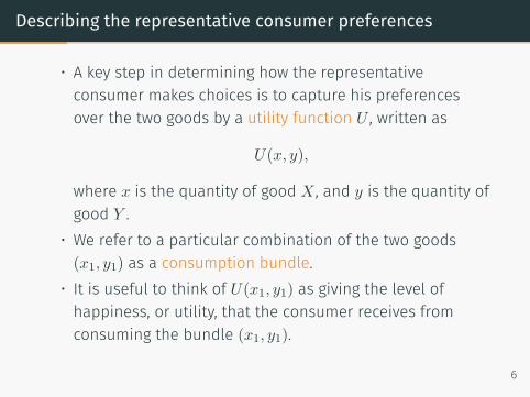
• A key step in determining how the representativeconsumer makes choices is to capture his preferencesover the two goods by a utility function U , written as
U(x, y),
where x is the quantity of good X , and y is the quantity ofgood Y .
• We refer to a particular combination of the two goods(x1, y1) as a consumption bundle.
• It is useful to think of U(x1, y1) as giving the level ofhappiness, or utility, that the consumer receives fromconsuming the bundle (x1, y1).
6
Utility functions as rankings for consumption bundles
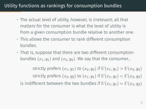
• The actual level of utility, however, is irrelevant; all thatmatters for the consumer is what the level of utility isfrom a given consumption bundle relative to another one.
• This allows the consumer to rank different consumptionbundles.
• That is, suppose that there are two different consumptionbundles (x1, y1) and (x2, y2). We say that the consumer…
strictly prefers (x1, y1) to (x2, y2) if U(x1, y1) > U(x2, y2)
strictly prefers (x2, y2) to (x1, y1) if U(x1, y1) < U(x2, y2)
is indifferent between the two bundles if U(x1, y1) = U(x2, y2)
7
Assumptions about preferences
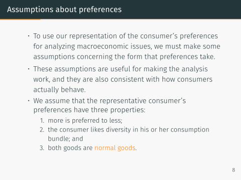
• To use our representation of the consumer’s preferencesfor analyzing macroeconomic issues, we must make someassumptions concerning the form that preferences take.
• These assumptions are useful for making the analysiswork, and they are also consistent with how consumersactually behave.
• We assume that the representative consumer’spreferences have three properties:
1. more is preferred to less;2. the consumer likes diversity in his or her consumption
bundle; and3. both goods are normal goods.
8
1. More is always preferred to less
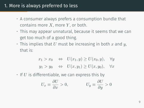
• A consumer always prefers a consumption bundle thatcontains more X , more Y , or both.
• This may appear unnatural, because it seems that we canget too much of a good thing.
• This implies that U must be increasing in both x and y,that is:
x1 > x0 ⇔ U(x1, y) ≥ U(x0, y), ∀yy1 > y0 ⇔ U(x, y1) ≥ U(x, y0), ∀x
• If U is differentiable, we can express this by
Ux ≡ ∂U
∂x> 0, Uy ≡ ∂U
∂y> 0
9

2. The consumer likes diversity in his bundle
• If the representative consumer is indifferent between twobundles with different combinations of X and Y , apreference for diversity means that any mixture of the twobundles is preferable to either one.
• In terms of the utility function:
U(x0, y0) = U(x1, y1) ⇒U(αx0 + (1− α)x1, αy0 + (1− α)y1) > U(x0, y0)
where 0 < α < 1.• If U satisfies this property, it is said to be strictlyquasiconcave.
10
3. Both goods are normal goods
• In some models, we will assume that both goods arenormal.
• A good is normal for a consumer if the quantity of thegood that he purchases increases when income increases.
• In contrast, a good is inferior for a consumer if hepurchases less of that good when income increases.
11

The utility function
• A consumer’s preferences over two goods x and y aredefined by the utility function
U(x, y)
• The U(, ) function is increasing in both goods, strictlyquasiconcave, and twice differentiable.
12
Indifference curves
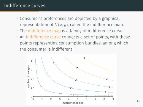
• Consumer’s preferences are depicted by a graphicalrepresentation of U(x, y), called the indifference map.
• The indifference map is a family of indifference curves.• An indifference curve connects a set of points, with thesepoints representing consumption bundles, among whichthe consumer is indifferent
1
1
1 12
2
23
3
3
4
4
5
0 1 2 3 4 5 6 7 8 9
number of apples
0
1
2
3
4
num
ber
of o
rang
es
13
The marginal rate of substitution
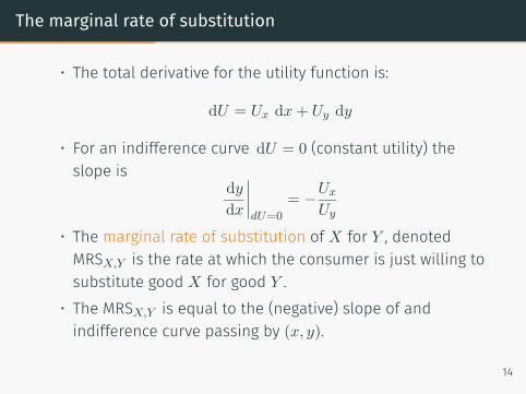
• The total derivative for the utility function is:
dU = Ux dx+ Uy dy
• For an indifference curve dU = 0 (constant utility) theslope is
dy
dx
∣∣∣∣dU=0
= −Ux
Uy
• The marginal rate of substitution of X for Y , denotedMRSX,Y is the rate at which the consumer is just willing tosubstitute good X for good Y .
• The MRSX,Y is equal to the (negative) slope of andindifference curve passing by (x, y).
14
Properties of an indifference curve
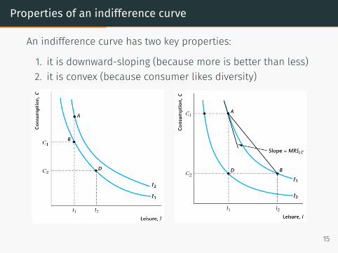
An indifference curve has two key properties:
1. it is downward-sloping (because more is better than less)2. it is convex (because consumer likes diversity)
15

Feasible bundles and budgetconstraints
The budget constraint
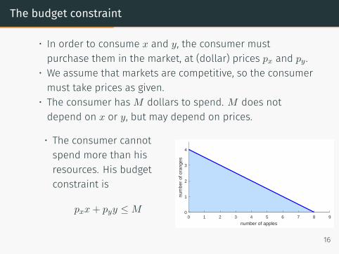
• In order to consume x and y, the consumer mustpurchase them in the market, at (dollar) prices px and py .
• We assume that markets are competitive, so the consumermust take prices as given.
• The consumer has M dollars to spend. M does notdepend on x or y, but may depend on prices.
• The consumer cannotspend more than hisresources. His budgetconstraint is
pxx+ pyy ≤ M0 1 2 3 4 5 6 7 8 9
number of apples
0
1
2
3
4
num
ber
of o
rang
es
16

Relative price
• Solving the budget constraint for y we have
y =M
py− px
pyx
• So the slope of the budget constraint is −pxpy: the
(negative) relative price of X in terms of Y .• The relative price X in terms of Y represents the numberof units of Y that a consumer must forfeit in order to getan additional unit of X .
17
A barter economy
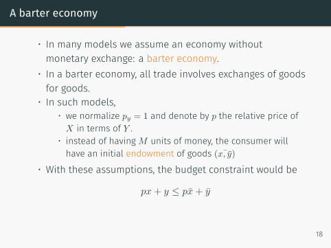
• In many models we assume an economy withoutmonetary exchange: a barter economy.
• In a barter economy, all trade involves exchanges of goodsfor goods.
• In such models,• we normalize py = 1 and denote by p the relative price ofX in terms of Y .
• instead of having M units of money, the consumer willhave an initial endowment of goods ( ¯x, y)
• With these assumptions, the budget constraint would be
px+ y ≤ px+ y
18

The representative consumerproblem
The consumers problem
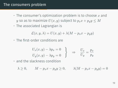
• The consumer’s optimization problem is to choose x andy so as to maximize U(x, y) subject to pxx+ pyy ≤ M
• The associated Lagrangian is
L(x, y, λ) = U(x, y) + λ(M − pxx− pyy)
• The first-order conditions are
Ux(x, y)− λpx = 0
Uy(x, y)− λpy = 0
}⇒ Ux
Uy=
pxpy
• and the slackness condition
λ ≥ 0, M − pxx− pyy ≥ 0, λ(M − pxx− pyy) = 0
19
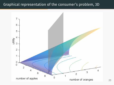
Graphical representation of the consumer’s problem, 3D
20
Don’t leave anything on the table
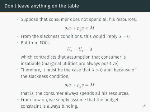
• Suppose that consumer does not spend all his resources:
pxx+ pyy < M
• From the slackness conditions, this would imply λ = 0.• But from FOCs,
Ux = Uy = 0
which contradicts that assumption that consumer isinsatiable (marginal utilities are always positive).
• Therefore, it must be the case that λ > 0 and, because ofthe slackness condition,
pxx+ pyy = M
that is, the consumer always spends all his resources.• From now on, we simply assume that the budgetconstraint is always binding. 21

Marshallian demand
• Dividing one FOC by the other we get that the solutionx∗, y∗ must satisfy
Ux(x∗, y∗)
Uy(x∗, y∗)=
pxpy
(MgRS = relative price)
pxx∗ + pyy
∗ = M (spend all resources)
• The solution values will depend on prices and income:
x∗ = x∗(px, py,M) y∗ = y∗(px, py,M)
• We refer to these functions as the Marshallian demandfunctions for X and Y .
22
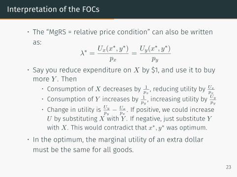
Interpretation of the FOCs
• The “MgRS = relative price condition” can also be writtenas:
λ∗ =Ux(x
∗, y∗)
px=
Uy(x∗, y∗)
py
• Say you reduce expenditure on X by $1, and use it to buymore Y . Then
• Consumption of X decreases by 1px, reducing utility by Ux
px
• Consumption of Y increases by 1py, increasing utility by Uy
py
• Change in utility is Uy
py− Ux
px. If positive, we could increase
U by substituting X with Y . If negative, just substitute Y
with X . This would contradict that x∗, y∗ was optimum.
• In the optimum, the marginal utility of an extra dollarmust be the same for all goods.
23
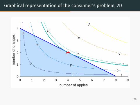
Graphical representation of the consumer’s problem, 2D
0 1 2 3 4 5 6 7 8 9
number of apples
0
1
2
3
4
num
ber
of o
rang
es
1
1
1 1
2
2
2
3
3
34
45
24
Indirect utility
• U(x, y) is defined over the set of consumption bundlesand represents the consumer’s preference directly, so wecall it the direct utility function
• Given prices and income, the consumer chooses autility-maximizing bundle (x∗, y∗).
• The level of utility achieved when this bundle is chosen isthe highest level permitted by the budget constraint. Itchanges when prices or income change.
• We define the indirect utility function as
V (px, py,M) = maxx,y
{U(x, y) s.t. pxx+ pyy = M}
= U (x∗(px, py,M), y∗(px, py,M))
25

An envelope condition
• Let’s say you need to compute the partial derivatives ofthe Lagrangian wrt income and prices. Then
L = U(x∗, y∗) + λ∗(M − pxx∗ − pyy
∗)
∂L∂M
= λ∗ + (Ux − λ∗px)∂x∗
∂M+ (Uy − λ∗py)
∂y∗
∂M= λ∗
∂L∂px
= −λ∗x∗ + (Ux − λ∗px)∂x∗
∂px+ (Uy − λ∗py)
∂y∗
∂px= −λ∗x∗
∂L∂py
= −λ∗y∗ + (Ux − λ∗px)∂x∗
∂py+ (Uy − λ∗py)
∂y∗
∂py= −λ∗y∗
• That is, we can derive the Lagrangian wrt the parametersas if x∗ and y∗ did not depend on those parameters!
26

The shadow price of income
• Remember that at optimum λ∗ = Uxpx
=Uy
py
• Let’s obtain the marginal value of an extra unit of income:∂V (px, py,M)
∂M=
∂U (x∗, y∗)
∂M
= Ux∂x∗
∂M+ Uy
∂y∗
∂M
= λ∗px∂x∗
∂M+ λ∗py
∂y∗
∂M
= λ∗(px
∂x∗
∂M+ py
∂y∗
∂M
)= λ∗ (because of budget constraint)
• That is, λ∗ represents the marginal utility of an extra unitof income.
27

Roy’s identity
• It is easy to obtain the indirect utility function from theMarshallian demand functions: we just substitute theMarshallian demands into the direct utility function.
• To obtain the Marshallian demand functions from theindirect utility function, we use Roy’s identity:
x∗ = −∂V∂px∂V∂M
y∗ = −∂V∂py∂V∂M
where we assume that V is differentiable and ∂V∂M = 0
28

A strictly positive monotone transformation
• Suppose that you rescale the utility function using astrictly increasing function f , where f ′(·) > 0
• That is, you use
W (x, y) ≡ f(U(x, y))
• Notice that the MRS is just the same as before:Wx
Wy=
f ′(U)Ux
f ′(U)Uy=
Ux
Uy
• So the optimal consumption bundle will be the same.• Utility function has ordinal meaning, but no cardinalmeaning.
• Warning: This result does not apply to choice problemswith uncertainty.
29
The consumers problem with non-negativity constraints
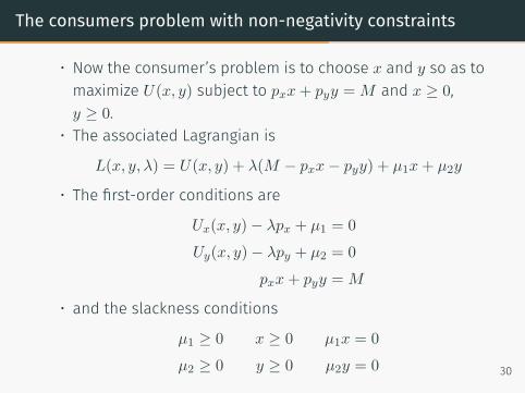
• Now the consumer’s problem is to choose x and y so as tomaximize U(x, y) subject to pxx+ pyy = M and x ≥ 0,y ≥ 0.
• The associated Lagrangian is
L(x, y, λ) = U(x, y) + λ(M − pxx− pyy) + µ1x+ µ2y
• The first-order conditions are
Ux(x, y)− λpx + µ1 = 0
Uy(x, y)− λpy + µ2 = 0
pxx+ pyy = M
• and the slackness conditions
µ1 ≥ 0 x ≥ 0 µ1x = 0
µ2 ≥ 0 y ≥ 0 µ2y = 0 30

• Notice that we can solve for µ1 and µ2 in the FOCs.
Ux(x, y)− λpx = −µ1
Uy(x, y)− λpy = −µ2
• So a solution must satisfy
Ux(x, y)− λpx ≤ 0 x ≥ 0 x (Ux(x, y)− λpx) = 0
Uy(x, y)− λpy ≤ 0 y ≥ 0 y (Uy(x, y)− λpy) = 0
pxx+ pyy = M
31
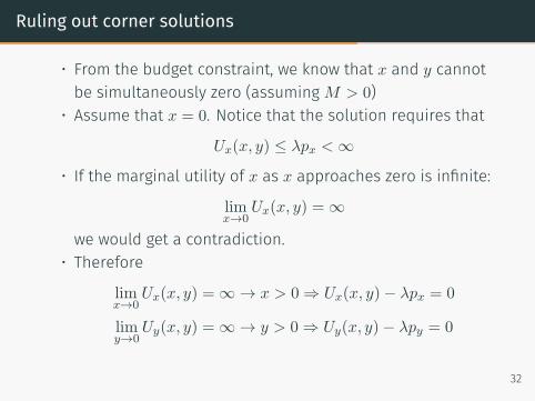
Ruling out corner solutions
• From the budget constraint, we know that x and y cannotbe simultaneously zero (assuming M > 0)
• Assume that x = 0. Notice that the solution requires that
Ux(x, y) ≤ λpx < ∞
• If the marginal utility of x as x approaches zero is infinite:
limx→0
Ux(x, y) = ∞
we would get a contradiction.• Therefore
limx→0
Ux(x, y) = ∞ → x > 0 ⇒ Ux(x, y)− λpx = 0
limy→0
Uy(x, y) = ∞ → y > 0 ⇒ Uy(x, y)− λpy = 0
32
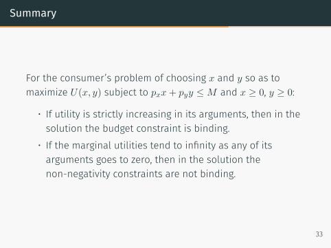
Summary
For the consumer’s problem of choosing x and y so as tomaximize U(x, y) subject to pxx+ pyy ≤ M and x ≥ 0, y ≥ 0:
• If utility is strictly increasing in its arguments, then in thesolution the budget constraint is binding.
• If the marginal utilities tend to infinity as any of itsarguments goes to zero, then in the solution thenon-negativity constraints are not binding.
33

Examples

Example 1:
A Cobb-Douglas utility function

• The Cobb-Douglas utility function is
U(x, y) = xθy1−θ (where 0 < θ < 1)
• The marginal utilities of x and y are
∂U
∂x= θ
(yx
)1−θ ∂U
∂y= (1− θ)
(x
y
)θ
• If x > 0 and y > 0, we have
limx→0
Ux = ∞ limy→0
Uy = ∞ Ux > 0 Uy > 0
• Therefore, if the utility is Cobb-Douglas, we know that• there will be no corner solution (x∗ > 0 and y∗ > 0).• the consumer will spend all his resources(pxx∗ + pyy
∗ = M )
34
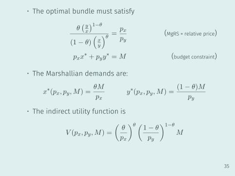
• The optimal bundle must satisfy
θ( yx
)1−θ
(1− θ)(xy
)θ =pxpy
(MgRS = relative price)
pxx∗ + pyy
∗ = M (budget constraint)
• The Marshallian demands are:
x∗(px, py,M) =θM
pxy∗(px, py,M) =
(1− θ)M
py
• The indirect utility function is
V (px, py,M) =
(θ
px
)θ (1− θ
py
)1−θ
M
35

Example 2:
A quasi-linear utility function
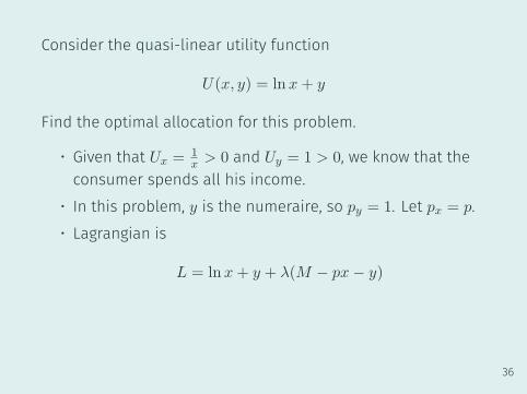
Consider the quasi-linear utility function
U(x, y) = lnx+ y
Find the optimal allocation for this problem.
• Given that Ux = 1x > 0 and Uy = 1 > 0, we know that the
consumer spends all his income.• In this problem, y is the numeraire, so py = 1. Let px = p.• Lagrangian is
L = lnx+ y + λ(M − px− y)
36
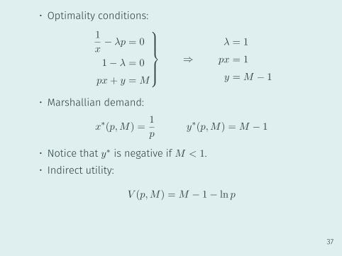
• Optimality conditions:
1
x− λp = 0
1− λ = 0
px+ y = M
⇒λ = 1
px = 1
y = M − 1
• Marshallian demand:
x∗(p,M) =1
py∗(p,M) = M − 1
• Notice that y∗ is negative if M < 1.• Indirect utility:
V (p,M) = M − 1− ln p
37

Example 3:
A quasi-linear utility function,with non-negativity constraints
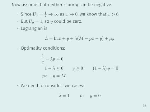
Now assume that neither x nor y can be negative.
• Since Ux = 1x → ∞ as x → 0, we know that x > 0.
• But Uy = 1, so y could be zero.• Lagrangian is
L = lnx+ y + λ(M − px− y) + µy
• Optimality conditions:1
x− λp = 0
1− λ ≤ 0 y ≥ 0 (1− λ) y = 0
px+ y = M
• We need to consider two cases:
λ = 1 or y = 0
38

Case 1: λ = 1
From FOC wrt x, we have λ−1 = px. So, in this case, px = 1.Substitute in the budget constraint to get
y∗ = M − 1 and x∗ =1
p
But we need to make sure that y ≥ 0, so we require that M ≥ 1.
39
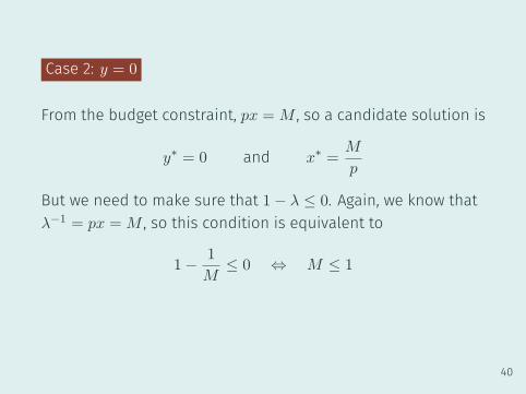
Case 2: y = 0
From the budget constraint, px = M , so a candidate solution is
y∗ = 0 and x∗ =M
p
But we need to make sure that 1− λ ≤ 0. Again, we know thatλ−1 = px = M , so this condition is equivalent to
1− 1
M≤ 0 ⇔ M ≤ 1
40

Taking the two cases together, we have the solution:
• Marshallian demand
x∗ =min{M, 1}
p, y∗ = max{M − 1, 0}
• Indirect utility
V (p,M) = max{M, 1} − 1 + lnmin{M, 1} − ln p
=
{lnM − ln p, if M ≤ 1
M − 1− ln p, otherwise
• Notice that V is continuous and differentiable at M = 1.
41

Example 4:
Many goods, CES utility

• Now assume that there are n+ 1 goods available to theconsumer.
• Let pi and xi be the price and quantity consumed of goodXi, for i = 0, 1, . . . , n.
• Assume a CES utility function, with αi > 0 ∀i
U(x0, x1, . . . , xn) =
(n∑
i=0
αixρi
) 1ρ
= (α0xρ0 + α1x
ρ1 + · · ·+ αnx
ρn)
1ρ
• Let X0 be the numeraire (p0 = 1) and let α0 = 1.• Budget constraint is
n∑i=0
pixi = p0x0 + p1x1 + · · ·+ pnxn = M
42
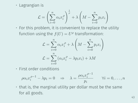
• Lagrangian is
L =
(n∑
i=0
αixρi
) 1ρ
+ λ
(M −
n∑i=0
pixi
)• For this problem, it is convenient to replace the utilityfunction using the f(U) = Uρ transformation:
L =
n∑i=0
αixρi + λ
(M −
n∑i=0
pixi
)
L =
n∑i=0
(αixρi − λpixi) + λM
• First order conditions
ραixρ−1i − λpi = 0 ⇒ λ =
ραixρ−1i
pi∀i = 0, . . . , n
• that is, the marginal utility per dollar must be the samefor all goods.
43
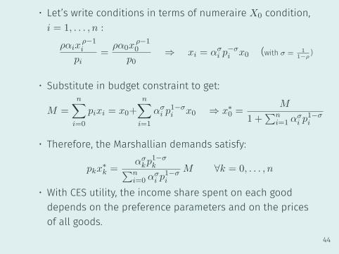
• Let’s write conditions in terms of numeraire X0 condition,i = 1, . . . , n :
ραixρ−1i
pi=
ρα0xρ−10
p0⇒ xi = ασ
i p−σi x0 (with σ = 1
1−ρ)
• Substitute in budget constraint to get:
M =
n∑i=0
pixi = x0+
n∑i=1
ασi p
1−σi x0 ⇒ x∗0 =
M
1 +∑n
i=1 ασi p
1−σi
• Therefore, the Marshallian demands satisfy:
pkx∗k =
ασkp
1−σk∑n
i=0 ασi p
1−σi
M ∀k = 0, . . . , n
• With CES utility, the income share spent on each gooddepends on the preference parameters and on the pricesof all goods.
44
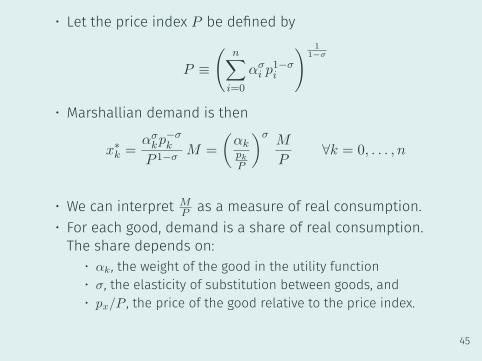
• Let the price index P be defined by
P ≡
(n∑
i=0
ασi p
1−σi
) 11−σ
• Marshallian demand is then
x∗k =ασkp
−σk
P 1−σM =
(αkpkP
)σ M
P∀k = 0, . . . , n
• We can interpret MP as a measure of real consumption.
• For each good, demand is a share of real consumption.The share depends on:
• αk , the weight of the good in the utility function• σ, the elasticity of substitution between goods, and• px/P , the price of the good relative to the price index.
45
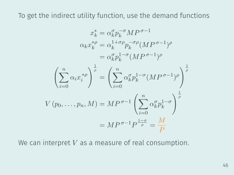
To get the indirect utility function, use the demand functions
x∗k = ασkp
−σk MP σ−1
αkx∗ρk = α1+σρ
k p−σρk (MP σ−1)ρ
= ασkp
1−σk (MP σ−1)ρ(
n∑i=0
αix∗ρi
) 1ρ
=
(n∑
i=0
ασkp
1−σk (MP σ−1)ρ
) 1ρ
V (p0, . . . , pn,M) = MP σ−1
(n∑
i=0
ασkp
1−σk
) 1ρ
= MP σ−1P1−σρ =
M
P
We can interpret V as a measure of real consumption.
46

• Case: Cobb-Douglas utility function is the special case
where ρ = 0 (equivalently σ = 1):
U(x0, x1, . . . , xn) =
n∏i=0
xαii = xα0
0 xα11 · · ·xαn
n
• In this case, the Marshallian demands satisfy:
pix∗i =
αi∑ni=0 αi
M ∀i = 0, . . . , n
• With Cobb-Douglas utility, the share of income spent oneach of the goods does not depend on any price.
47

References
Jehle, Geoffrey A. and Philip J. Reny (2001). AdvancedMicroeconomic Theory. 2nd ed. Addison Wesley. isbn:978-0321079169.
Williamson, Stephen D. (2014). Macroeconomics. 5th ed.Pearson.
48