lecture 8: inequality (mixed) constraints, karusch- kuhn
TRANSCRIPT
Copyright ©1991-2009 by K. Pattipati1
Lecture 8: Inequality (mixed) Constraints,
Karusch- Kuhn-Tucker Conditions,
Convex Programming,Primal-Dual Methods
Prof. Krishna R. Pattipati
Dept. of Electrical and Computer Engineering
University of Connecticut Contact: [email protected] (860) 486-2890
Fall 2009
October 20, 2009
ECE 6437Computational Methods for Optimization
Copyright ©1991-2009 by K. Pattipati2
Outline of Lecture 8
Lagrange Multipliers and Duality
Inequality (Mixed) Constraints
Karusch-Kuhn-Tucker (KKT) Conditions
Illustrative Examples
Convex Programming and Duality
Saddle Point Theorem
Primal-Dual Methods

Copyright ©1991-2009 by K. Pattipati3
Second-order conditions
What do λs mean ?
* * *
*
min ( ) ( ) ( ) 0
s.t. ( ) 0 ( ) 0
f x f x h x
h x h x
Review of Optimality Conditions - 1
2 * 2 * *
1
( ) ( ) 0 ( ) 0 1,2,...,m
TT
ii i
i
y f x h x y h x y i m
First order
Conditions
*
Consider min ( )
s.t. ,
Suppose
x
T
T
T
f x
a x b
b b b
a x x b b
a x b
*Ta x x b b
*Ta x b
*x x
x*x
Copyright ©1991-2009 by K. Pattipati4
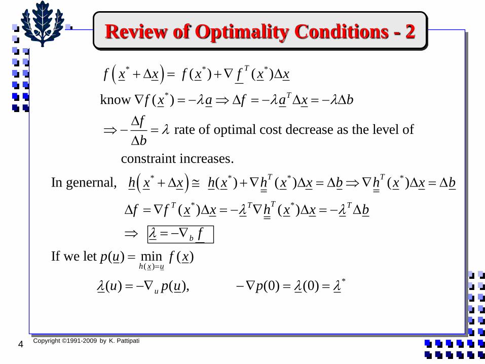
* * *
*
( ) ( )
know ( )
rate of optimal cost decrease as the level of
constraint increases.
In gener
T
T
f x x f x f x x
f x a f a x b
f
b
* * * *
* *
( )
nal, ( ) ( ) ( )
( ) ( )
If we let ( ) min ( )
( ) ( ), (0)
T T
TT T T
b
h x u
u
h x x h x h x x b h x x b
f f x x h x x b
f
p u f x
u p u p
*(0)
Review of Optimality Conditions - 2
Copyright ©1991-2009 by K. Pattipati5
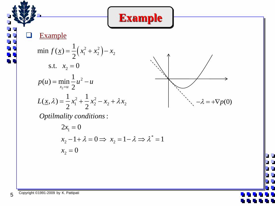
Example
2
2 2
1 2 2
2
2
2 2
1 2 2 2
1
*
2 2
2
1min ( )
2
s.t. 0
1( ) min
2
1 1( , )
2 2
:
2 0
1 0 1 1
0
x u
f x x x x
x
p u u u
L x x x x x
Optilmality conditions
x
x x
x
Example
(0)p
Copyright ©1991-2009 by K. Pattipati6
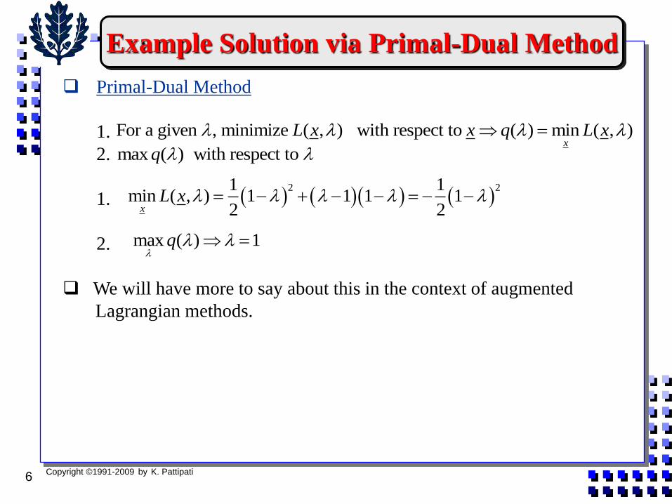
Primal-Dual Method
1.
2.
1.
2.
We will have more to say about this in the context of augmented
Lagrangian methods.
Example Solution via Primal-Dual Method
For a given , minimize ( , ) with respect to ( ) min ( , )x
L x x q L x
max ( ) with respect to q
2 21 1
min ( , ) 1 1 1 12 2x
L x
max ( ) 1q
Copyright ©1991-2009 by K. Pattipati7
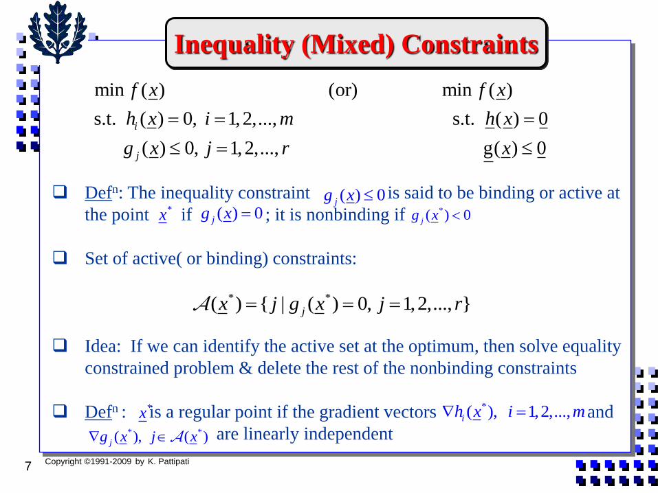
Defn: The inequality constraint is said to be binding or active at
the point if ; it is nonbinding if
Set of active( or binding) constraints:
Idea: If we can identify the active set at the optimum, then solve equality
constrained problem & delete the rest of the nonbinding constraints
Defn : is a regular point if the gradient vectors and
are linearly independent
min ( ) (or) min ( )
s.t. ( ) 0, 1,2,..., s.t. ( ) 0
( ) 0, 1,2,...,
i
j
f x f x
h x i m h x
g x j r
g( ) 0x
Inequality (Mixed) Constraints
( ) 0jg x *x ( ) 0jg x *( ) 0jg x
* *( ) { | ( ) 0, 1,2,..., }jx j g x j r
*x*( ), 1,2,...,ih x i m
* *( ), ( )jg x j x
Copyright ©1991-2009 by K. Pattipati8
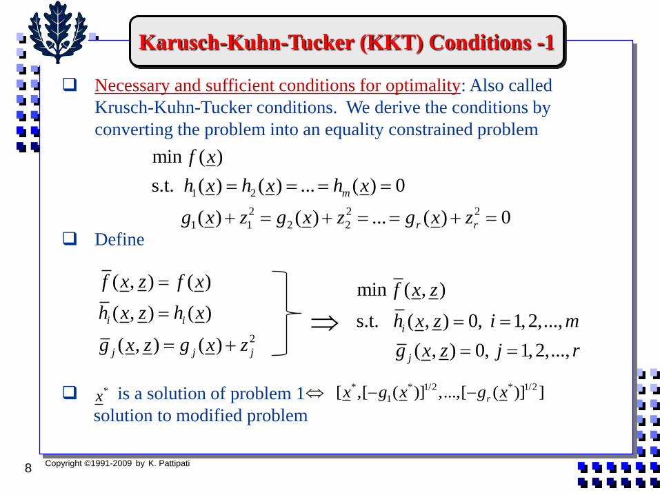
Necessary and sufficient conditions for optimality: Also called
Krusch-Kuhn-Tucker conditions. We derive the conditions by
converting the problem into an equality constrained problem
Define
is a solution of problem 1
solution to modified problem
Karusch-Kuhn-Tucker (KKT) Conditions -1
* * 1/2 * 1/2
1 [ ,[ ( )] ,...,[ ( )] ]rx g x g x
2
( , ) ( )
( , ) ( )
( , ) ( )
i i
j j j
f x z f x
h x z h x
g x z g x z
min ( , )
s.t. ( , ) 0, 1,2,...,
( , ) 0, 1,2,...,
i
j
f x z
h x z i m
g x z j r
*x
1 2
2 2 2
1 1 2 2
min ( )
s.t. ( ) ( ) ... ( ) 0
( ) ( ) ... ( ) 0
m
r r
f x
h x h x h x
g x z g x z g x z

Copyright ©1991-2009 by K. Pattipati9
Binding inequality constraint * 0jz
*
* *
*
* *
*
( ) ( )
00
.., ( , ) , 1, 2,...,
..
..
00
( )
0
.( , ) ; 1, 2,...,
.
2
0
i
i
j
j
j
f x h x
f h x z i m
g x
g x z j r
z
n
n j
Karusch-Kuhn-Tucker (KKT) Conditions - 2
Copyright ©1991-2009 by K. Pattipati10
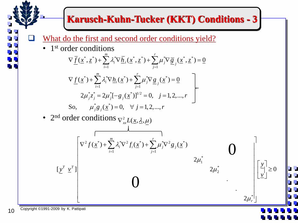
What do the first and second order conditions yield?
• 1st order conditions
• 2nd order conditions
* * * * * * * *
1 1
* * * * *
1 1
* * * * 1/2
* *
( , ) ( , ) ( , ) 0
( ) ( ) ( ) 0
2 2 [ ( )] 0, 1,2,...,
So, ( ) 0, 1,2,...,
m r
ii j ji j
m r
ii j ji j
j j j j
j j
f x z h x z g x z
f x h x g x
z g x j r
g x j r
2 * * 2 * * 2 *
1 1
*
1
*
2
*
( ) ( ) ( )
2
[ ] 02
.
.
2
m r
i i j j
i j
T T
r
f x f x g x
yy v
v
2 ( , , )xxL x
0
0
Karusch-Kuhn-Tucker (KKT) Conditions - 3
Copyright ©1991-2009 by K. Pattipati11
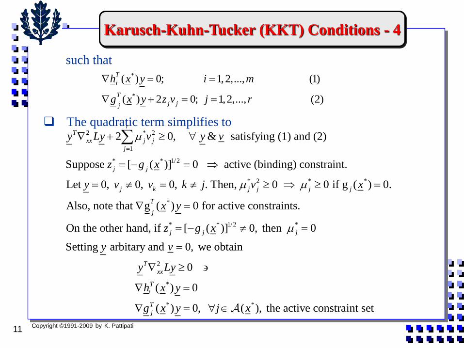
such that
The quadratic term simplifies to
*
*
( ) 0; 1,2,..., (1)
( ) 2 0; 1,2,..., (2)
T
i
T
j jj
h x y i m
g x y z v j r
2 * 2
1
* * 1/2
* 2 * *
*
2 0, & satisfying (1) and (2)
Suppose [ ( )] 0 active (binding) constraint.
Let 0, 0, 0, . Then, 0 0 if g ( ) 0.
Also, note that g ( )
rT
xx j j
j
j j
j k j j j j
T
j
y Ly v y v
z g x
y v v k j v x
x
* * 1/2 *
2
*
0 for active constraints.
On the other hand, if [ ( )] 0, then 0
Setting arbitary and 0, we obtain
0
( ) 0
j j j
T
xx
T
i
y
z g x
y v
y Ly
h x y
* * ( ) 0, ( ), the active constraint setT
jg x y j x
Karusch-Kuhn-Tucker (KKT) Conditions - 4
Copyright ©1991-2009 by K. Pattipati12
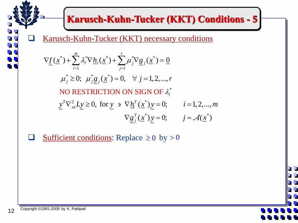
Karusch-Kuhn-Tucker (KKT) necessary conditions
Sufficient conditions: Replace by
* * * * *
1 1
* * *
*
2 *
NO RESTRICTION ON SIGN
( ) ( ) ( ) 0
0; ( ) 0, 1,2,...,
0, for ( ) 0; 1,2,...,
OF
m r
ii j j
i j
j j j
i
T T
xx i
f x h x g x
g x j r
y Ly y h x y i m
* * ( ) 0; ( )T
jg x y j x
0 0
Karusch-Kuhn-Tucker (KKT) Conditions - 5

Copyright ©1991-2009 by K. Pattipati13
Example 2 2 2
1 2 3
1 2 3
* *
1 1
* *
2 1
* *
3 1
*
1 1 2 3
*
1
1 min ( )
2
s.t. 3
:
0
0
Necessary conditions
0
( 3) 0
0
x x x
x x x
x
x
x
x x x
* * * * * * *
1 2 3 1 1 2 3
* * * * * * *
1 2 3 1 1 2 3
n
2
1 2 3 1 2
: 3 0 0 3, contradiction
: 3 1, 1
Second order cond
0 0
case 1
case 2
T
x x x x x x
x x x x x x
y y y y y y y y
2 2
1 2 1 2
*
( ) 0 non-zero ,
so, is a strict local minimum (& a global minimum as well)
y y y y
x
Illustration of Optimality Conditions - 1
Copyright ©1991-2009 by K. Pattipati14
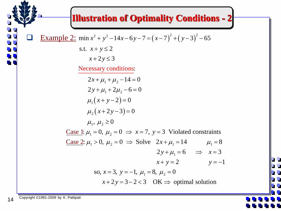
Example 2:
2 22 2
1 2
1 2
1
2
Necessary conditio
min 14 6 7 7 3 65
s.t. 2
2 3
:
2 14 0
2 2 6 0
2 0
2 3
ns
x y x y x y
x y
x y
x
y
x y
x y
1 2
1 2
1 2 1 1
1
0
, 0
: 0, 0 7, 3 Violated constraints
: 0, 0 Solve 2 14 8
Case 1
C
ase
2 6
2
3
x y
x
y x
1 2
2 1
so, 3, 1, 8, 0
2 3 2 3 OK optimal solution
x y y
x y
x y
Illustration of Optimality Conditions - 2
Copyright ©1991-2009 by K. Pattipati15
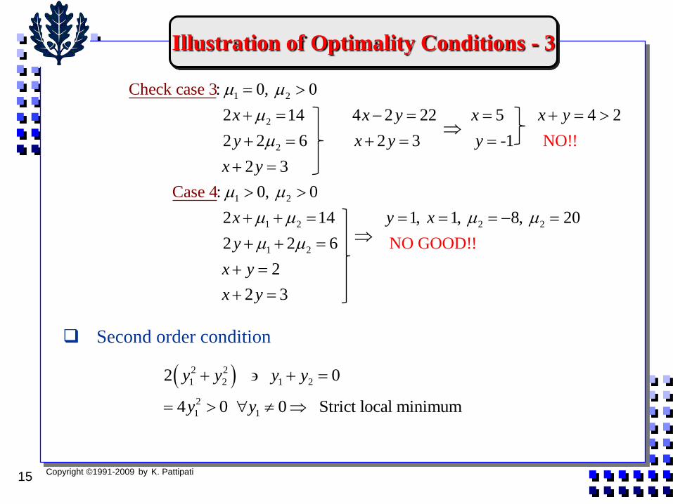
Second order condition
1 2
2
2
: 0, 0
2 14 4 2 22 5 4 2
2 2 6 2 3
C
-1
heck ca
se
NO
3
!
!
x x y x x y
y x y y
x
1 2
1 2 2 2
1 2
2 3
: 0, 0
2 14 1, 1, 8, 20
2 2 6
Case
NO GOOD!!
2
4
y
x y x
y
x y
2 3 x y
2 2
1 2 1 2
2
1 1
2 0
4 0 0 Strict local minimum
y y y y
y y
Illustration of Optimality Conditions - 3
Copyright ©1991-2009 by K. Pattipati16
Second order condition
2 2
1 2 1 2 2
2
1 1
2 0 & 0
2 0 0 Strict local minimum
y y y y y
y y
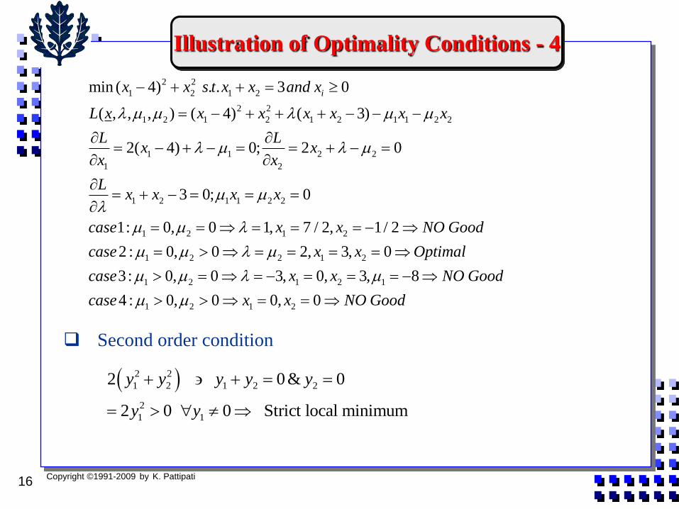
Illustration of Optimality Conditions - 4
2 2
1 2 1 2
2 2
1 2 1 2 1 2 1 1 2 2
1 1 2 2
1 2
1 2 1 1 2 2
1 2 1 2
1 2
min ( 4) . . 3 0
( , , , ) ( 4) ( 3)
2( 4) 0; 2 0
3 0; 0
1: 0, 0 1, 7 / 2, 1/ 2
2 : 0, 0
ix x s t x x and x
L x x x x x x x
L Lx x
x x
Lx x x x
case x x NO Good
case
2 1 2
1 2 1 2 1
1 2 1 2
2, 3, 0
3: 0, 0 3, 0, 3, 8
4 : 0, 0 0, 0
x x Optimal
case x x NO Good
case x x NO Good
Copyright ©1991-2009 by K. Pattipati17
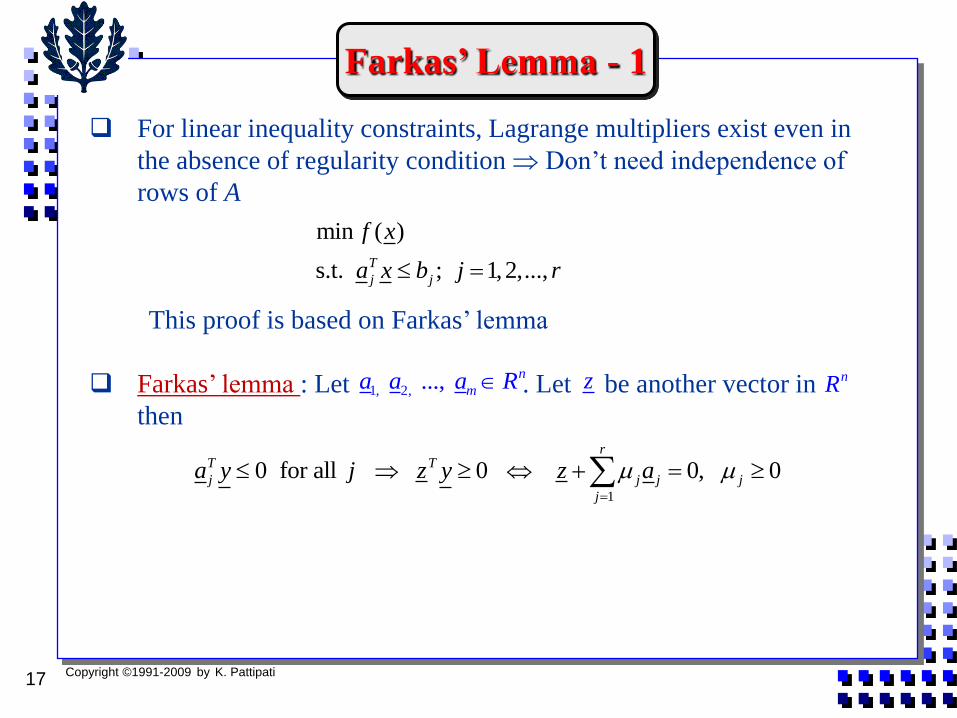
For linear inequality constraints, Lagrange multipliers exist even in
the absence of regularity condition Don’t need independence of
rows of A
This proof is based on Farkas’ lemma
Farkas’ lemma : Let . Let be another vector in
then
min ( )
s.t. ; 1,2,...,T
j j
f x
a x b j r
1, 2, ..., n
ma a a R z nR
1
0 for all 0 0, 0r
T T
j j j j
j
a y j z y z a
Farkas’ Lemma - 1
Copyright ©1991-2009 by K. Pattipati18
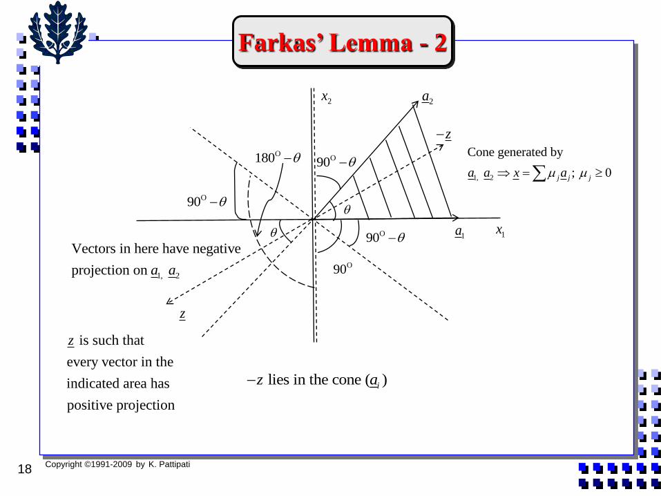
O90
2a
1a 1x
z
1, 2
Cone generated by
; 0j j ja a x a
O90
O90
O90
O180
1, 2
Vectors in here have negative
projection on a a
z
is such that
every vector in the
indicated area has
positive projection
z
2x
lies in the cone ( )iz a
Farkas’ Lemma - 2

Copyright ©1991-2009 by K. Pattipati19
*
* * *
*
* * *
Now consider min ( ) s.t. , ( )
From Nec. condition: ( )( ) 0, , ( )
since ( ) 0
Let ( ) ( ) 0, , ( )
From Farka's l
T
j j
T T
j j
T T
j j j
T T
j j
f x a x b j A x
f x x x x a x b j A x
a x b a x x
x x y f x y y a y b j A x
*
* *
( )
* * *
emma, ( ) 0
since 0 for ( ) ( ) 0
The result extends to equality constraints since
j j
j A x
T T
j
T
i i
T
i i
f x a
j A x f x A
c x d
c x d c
(or)
T
i i
T T
i i i i
x d
c x d c x d
Application of Farkas’ Lemma
Any equality constraint can be re-written as two inequality constraints

Copyright ©1991-2009 by K. Pattipati20
Convex programming problems and Duality
Geometric interpretation of Lagrange multiplier vector
Convex Programming and Duality-1
1
* *
* * * * *
min ( )
s.t. and ( ) 0, 1,2,...,
( ) convex, ( ) is convex and convex
Lagrangian ( , ) ( ) ( )
Also min ( , ) ( )
Since ( ) 0 ( ) ( )
j
j
r
j j
j
x
j j j j
f x
x g x j r
f x g x
L x f x g x
L x f x
g x f x f x g
* *
1 1
( ) min ( ) ( )r r
j jx
j j
x f x g x
* 1 is a Lagrange multiplier vector if and only if the set
of all possible pairs of ( ), ( ) as ranges over
( , ) | ( ), ( ),
rS R
g x f x x
S z w z g x w f x x
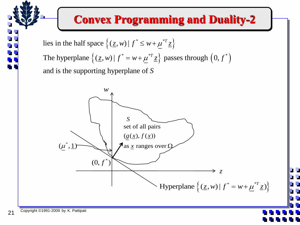
Copyright ©1991-2009 by K. Pattipati21
* *
* * *
lies in the half space ( , ) |
The hyperplane ( , ) | passes through 0,
and is the supporting hyperplane of
T
T
z w f w z
z w f w z f
S
**Hyperplane ( , ) | )T
z w f w z
set of all pairs
( ( ), ( ))
as ranges over
g x f x
x
w
S
*(0, )f
*( , 1)
z
Convex Programming and Duality-2
Copyright ©1991-2009 by K. Pattipati22
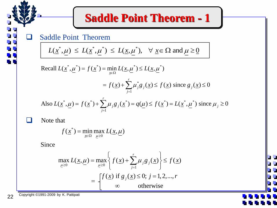
Saddle Point Theorem
Saddle Point Theorem - 1
* * * *( , ) ( , ) ( , ), and 0L x L x L x x
* * * * *
*
1
* * * * * *
1
Recall ( , ) ( ) min ( , ) ( , )
( ) ( ) ( ) since ( ) 0
Also ( , ) ( ) ( ) ( ) ( ) ( , ) since 0
x
r
j j j
j
r
j j j
j
L x f x L x L x
f x g x f x g x
L x f x g x q f x L x
*
0
0 01
Note that
( ) min max ( , )
Since
max ( , ) max ( ) ( ) ( )
( ) if ( ) 0; 1,2,...,
otherwise
x
r
j j
j
j
f x L x
L x f x g x f x
f x g x j r
Copyright ©1991-2009 by K. Pattipati23
*
0
* *
* *
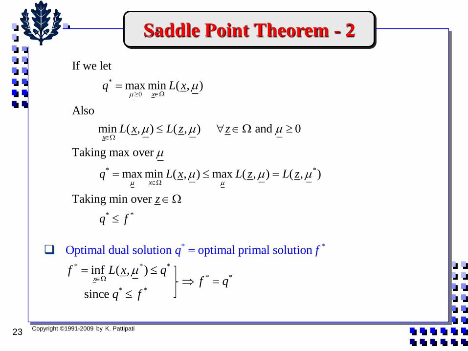
If we let
max min ( , )
Also
min ( , ) ( , ) and 0
Taking max over
max min ( , ) max ( , ) ( , )
Taking min over
x
x
x
q L x
L x L z z
q L x L z L z
z
q f
* *
* * *
* *
* *
Optimal dual solution optimal primal soluti
inf ( , )
si
on
nce
xf L x q
f qq
f
f
q
Saddle Point Theorem - 2
Copyright ©1991-2009 by K. Pattipati24
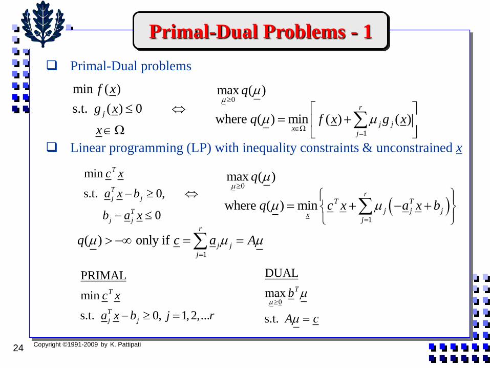
Primal-Dual Problems - 1
min ( )
s.t. ( ) 0
j
f x
g x
x
Primal-Dual problems
Linear programming (LP) with inequality constraints & unconstrained x
0max ( )q
1
where ( ) min ( ) ( )r
j jx
j
q f x g x
min
s.t. 0,
0
T
T
j j
T
j j
c x
a x b
b a x
0max ( )q
1
where ( ) minr
T T
j j jx
j
q c x a x b
1
( ) only if r
j j
j
q c a A
PRIMAL
min
s.t. 0, 1,2,...
T
T
j j
c x
a x b j r
0
DUAL
max
s.t.
Tb
A c
Copyright ©1991-2009 by K. Pattipati25
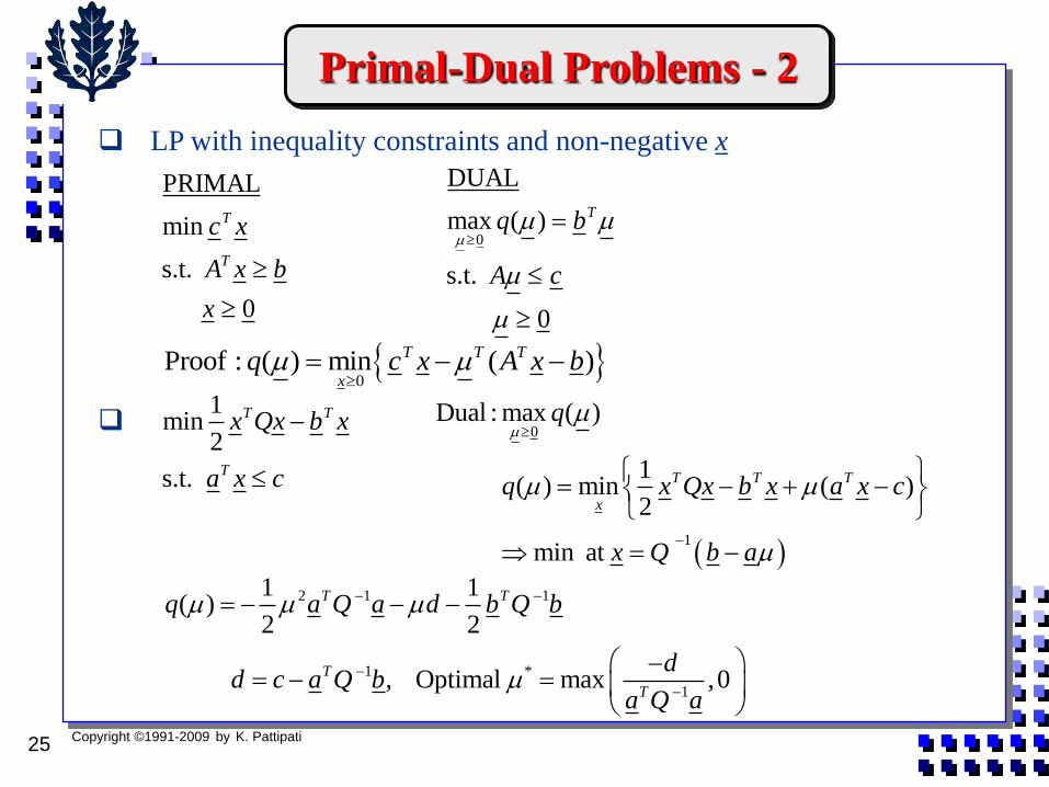
LP with inequality constraints and non-negative x
0
Proof : ( ) min ( )T T T
xq c x A x b
PRIMAL
min
s.t.
0
T
T
c x
A x b
x
0
DUAL
max ( )
s.t.
0
Tq b
A c
1min
2
s.t.
T T
T
x Qx b x
a x c
0
1
Dual : max ( )
1 ( ) min ( )
2
min at
T T T
x
q
q x Qx b x a x c
x Q b a
2 1 1
1 *
1
1 1( )
2 2
, Optimal max ,0
T T
T
T
q a Q a d b Q b
dd c a Q b
a Q a
Primal-Dual Problems - 2
Copyright ©1991-2009 by K. Pattipati26
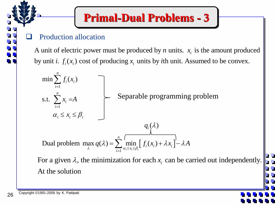
Production allocation
A unit of electric power must be produced by units. is the amount produced
by unit . ( ) cost of producing units by th unit. Assumed to be convex.
i
i i i
n x
i f x x i
1
1
min ( )
s.t.
n
i i
i
n
i
i
i i i
f x
x A
x
Separable programming problem
1
Dual problem max ( ) min ( )i i i
n
i i ix
i
q f x x A
( )iq
For a given , the minimization for each can be carried out independently.
At the solution
ix
Primal-Dual Problems - 3
Copyright ©1991-2009 by K. Pattipati27
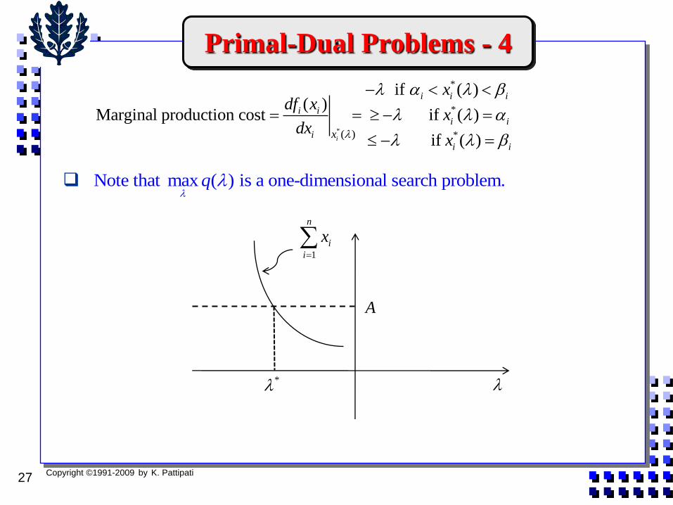
Note that max ( ) is a one-dimensional search problem.q
*
*
*
if ( ) ( )
Marginal production cost if ( )
if ( )
i i i
i ii i
i
i i
xdf x
xdx
x
*( )ix
1
n
i
i
x
A
*
Primal-Dual Problems - 4

Copyright ©1991-2009 by K. Pattipati28
Algorithm is well-suited for parallel implementation
Update λ
*( )nx *
2 ( )x *
1 ( )x
1
opt.
x 2
opt.
x
opt.
nx
• This algorithm works even
with asynchronous updates
Primal-Dual Problems - 5
Copyright ©1991-2009 by K. Pattipati29
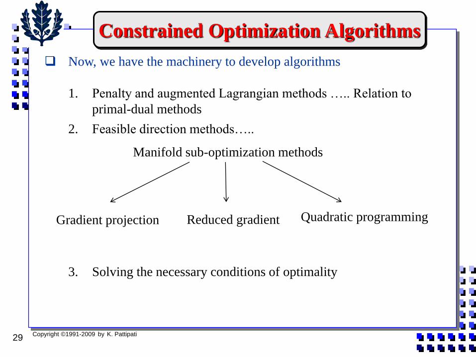
Now, we have the machinery to develop algorithms
1. Penalty and augmented Lagrangian methods ….. Relation to
primal-dual methods
2. Feasible direction methods…..
3. Solving the necessary conditions of optimality
Manifold sub-optimization methods
Gradient projection Reduced gradient Quadratic programming
Constrained Optimization Algorithms
Copyright ©1991-2009 by K. Pattipati30
Summary
Lagrange Multipliers and Duality
Inequality (Mixed) Constraints
Karusch-Kuhn-Tucker (KKT) Conditions
Illustrative Examples
Convex Programming and Duality
Saddle Point Theorem
Primal-Dual Methods