lecture 8: interest point detection - university of...
TRANSCRIPT


Review of Edge Detectors#2

Today’s Lecture
• Interest Points Detection
• What do we mean with Interest Point Detection in an Image
• Goal: Find Same features between multiple images taken from different position or time

Applications
• Image alignment • Image Stitching• 3D reconstruction• Object recognition• Indexing and database retrieval• Object tracking• Robot navigation

Image Alignment
• Homography• Ransac
#5

• What points would you choose?Known as:Template Matching Method, with option to use correlation as a metric

Correlation#7

Correlation
• Use Cross Correlation to find the template in an image, • Maximum indicate high similarity
#8


We need more robust feature descriptors for matching !!!!!

Interest Points
• Local features associated with a significant change of an image property of several properties simultaneously (e.g., intensity, color, texture).

Why Extract Interest Points?
• Corresponding points (or features) between images enable the estimation of parameters describing geometric transforms between the images.

What if we don’t know the correspondences?
• Need to compare feature descriptors of local patches surrounding interest points
( ) ( )=?feature
descriptorfeature
descriptor
?

Properties of good features• Local: features are local, robust to occlusion and
clutter (no prior segmentation!).• Accurate: precise localization.
• Invariant (or covariant)• Robust: noise, blur, compression, etc.
do not have a big impact on the feature.
• Distinctive: individual features can be matched to a large database of objects.
• Efficient: close to real-time performance.
Repeatable

Invariant / Covariant
• A function f( ) is invariant under some transformation T( ) if its value does change when the transformation is applied to its argument:
if f(x) = y then f(T(x))=y
• A function f( ) is covariant when it commutes with the transformation T( ):
if f(x) = y then f(T(x))=T(f(x))=T(y)

Invariance• Features should be detected despite geometric or
photometric changes in the image.• Given two transformed versions of the same
image, features should be detected in corresponding locations.

Example: Panorama Stitching
• How do we combine these two images?

Panorama stitching (cont’d)
Step 1: extract featuresStep 2: match features
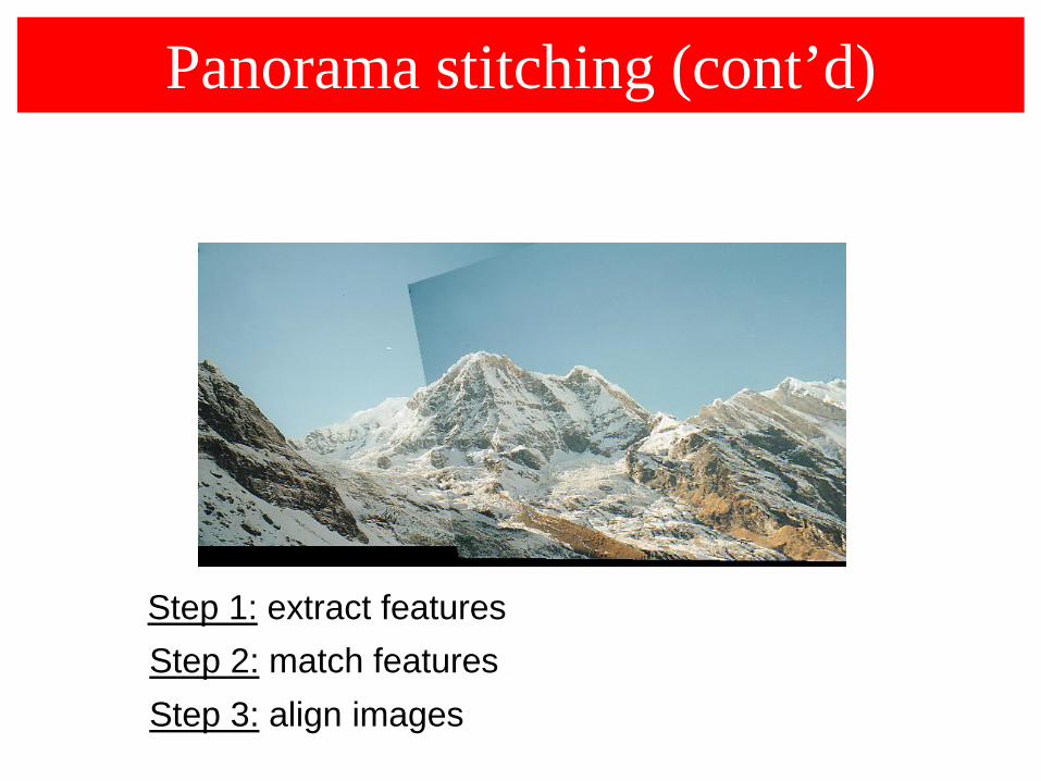
Panorama stitching (cont’d)
Step 1: extract featuresStep 2: match featuresStep 3: align images

What features should we use?
Use features with gradients in at least two (significantly) different orientations patches ? Corners ?

What features should we use? (cont’d)
(auto-correlation)

The Aperture Problem#23

Corners vs Edges#24

Corner Detection#25

Corner Detection-Basic Idea#26

Corner Detector: Basic Idea#27

Mains Steps in Corner Detection
1. For each pixel in the input image, the corner operator is appliedto obtain a cornerness measure for this pixel.
2. Threshold cornerness map to eliminate weak corners.3. Apply non-maximal suppression to eliminate points whose
cornerness measure is not larger than the cornerness values of all points within a certain distance.

Mains Steps in Corner Detection (cont’d)

Corner Types
Example of L-junction, Y-junction, T-junction, Arrow-junction, and X-junction corner types

Corner Detection Using Edge Detection?
• Edge detectors are not stable at corners.• Gradient is ambiguous at corner tip.• Discontinuity of gradient direction near
corner.

Corner Detection Using Intensity: Basic Idea
• Image gradient has two or more dominant directions near a corner.
• Shifting a window in any direction should give a large change in intensity.
“edge”: no change along the edge direction
“corner”: significant change in all directions
“flat” region:no change in all directions

Moravec Detector (1977)• Measure intensity variation at (x,y) by shifting a
small window (3x3 or 5x5) by one pixel in each of the eight principle directions (horizontally, vertically, and four diagonals).

Moravec Detector (1977)• Calculate intensity variation by taking the sum of squares
of intensity differences of corresponding pixels in these two windows.
∆x, ∆y in {-1,0,1}
SW(-1,-1), SW(-1,0), ...SW(1,1)
8 directions

Moravec Detector (cont’d)• The “cornerness” of a pixel is the minimum intensity variation
found over the eight shift directions:
Cornerness(x,y) = min{SW(-1,-1), SW(-1,0), ...SW(1,1)}
CornernessMap
(normalized)
Note response to isolated points!

Moravec Detector (cont’d)
• Non-maximal suppression will yield the final corners.

Moravec Detector (cont’d)
• Does a reasonable job infinding the majority of true corners.
• Edge points not in one of the eight principle directions will be assigned a relatively large cornerness value.

Moravec Detector (cont’d)• The response is anisotropic as the intensity variation
is only calculated at a discrete set of shifts (i.e., not rotationally invariant)
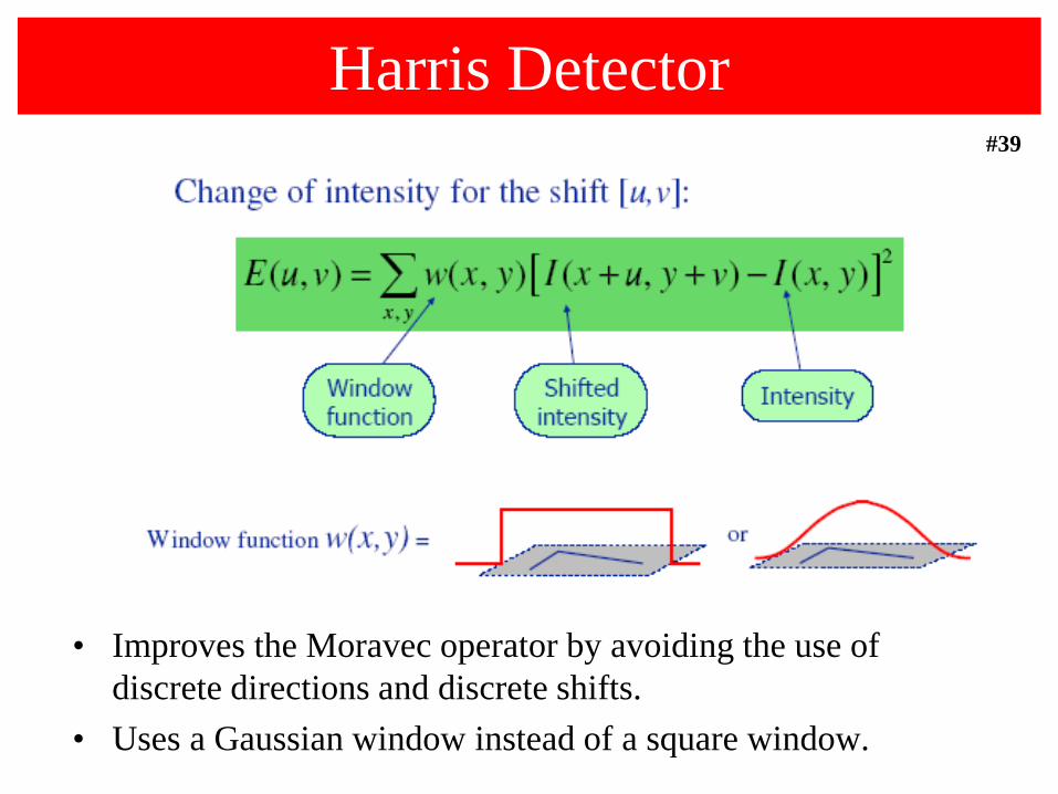
Harris Detector
• Improves the Moravec operator by avoiding the use of discrete directions and discrete shifts.
• Uses a Gaussian window instead of a square window.
#39

Harris Detector#40

Harris Detector (cont’d)
• Using first-order Taylor approximation:
Reminder: Taylor expansion += + − + − + + − +( )
2 1f´( ) f´´( ) f ( )( ) f( ) ( ) ( ) ( ) ( )1! 2! !
nn na a af x a x a x a x a O x
n

Harris Detector (cont’d)
Since

Harris Detector (cont’d)
2 x 2 matrix(auto-correlation or2nd order moment matrix)
2( , )( )i if x yx
∂∂
2( , )( )i if x yy
∂∂
AW(x,y)=

Harris Detector
[ ]2
,( , ) ( , ) ( , ) ( , )
i i
W i i i i i ix y
S x y w x y f x y f x x y y∆ ∆ = − −∆ −∆∑
default window function w(x,y) :
1 in window, 0 outside
• General case – use window function:
22
, ,2
,2
, ,
( , ) ( , )( , )
( , ) ( , )
x x yx y x y x x y
Wx y x y y
x y yx y x y
w x y f w x y f ff f f
A w x yf f f
w x y f f w x y f
= =
∑ ∑∑
∑ ∑

Harris Detector (cont’d)
window function w(x,y) :Gaussian
• Harris uses a Gaussian window: w(x,y)=G(x,y,σI) where σIis called the “integration” scale
22
, ,2
,2
, ,
( , ) ( , )( , )
( , ) ( , )
x x yx y x y x x y
Wx y x y y
x y yx y x y
w x y f w x y f ff f f
A w x yf f f
w x y f f w x y f
= =
∑ ∑∑
∑ ∑

Harris Detector
Describes the gradientdistribution (i.e., local structure)inside window!
Does not depend on
2
2,
x x yW
x y x y y
f f fA
f f f
=
∑
,x y∆ ∆

Harris Detector (cont’d)
Since M is symmetric, we have: 11
2
00WA R Rλ
λ−
=
We can visualize AW as an ellipse with axis lengths determined by the eigenvalues and orientation determined by R
(λmin)-1/2
(λmax)-1/2[ ] constW
xx y A
y∆
∆ ∆ = ∆
Ellipse equation:direction of the slowest change
direction of the fastest change

Harris Detector (cont’d)
• Eigenvectors encode edge direction
• Eigenvalues encode edge strength
(λmin)-1/2
(λmax)-1/2
direction of the fastest change
direction of the slowest change

Distribution of fx and fy
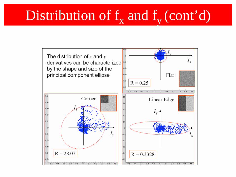
Distribution of fx and fy (cont’d)

Harris Detector (cont’d)
λ1
λ2
“Corner”λ1 and λ2 are large,λ1 ~ λ2;E increases in all directions
λ1 and λ2 are small;SW is almost constant in all directions
“Edge” λ1 >> λ2
“Edge” λ2 >> λ1
“Flat” region
Classification of image points using eigenvalues of AW :

Harris Detector (cont’d)
(assuming that λ1 > λ2)
λ2
%
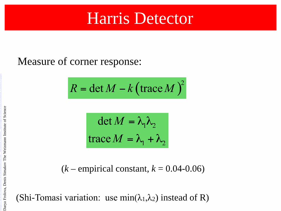
Harris Detector
Measure of corner response:
(k – empirical constant, k = 0.04-0.06)
(Shi-Tomasi variation: use min(λ1,λ2) instead of R)
http
://w
ww
.wis
dom
.wei
zman
n.ac
.il/~
deni
ss/v
isio
n_sp
ring0
4/fil
es/In
varia
ntFe
atur
es.p
ptD
arya
Fro
lova
, Den
is S
imak
ov T
he W
eizm
ann
Inst
itute
of S
cien
ce

Harris Detector: Mathematics
“Corner”
“Edge”
“Edge”
“Flat”
• R depends only on eigenvalues of M
• R is large for a corner
• R is negative with large magnitude for an edge
• |R| is small for a flatregion
R > 0
R < 0
R < 0|R| small

Harris Detector
• The Algorithm:– Find points with large corner response function
R (R > threshold)– Take the points of local maxima of R
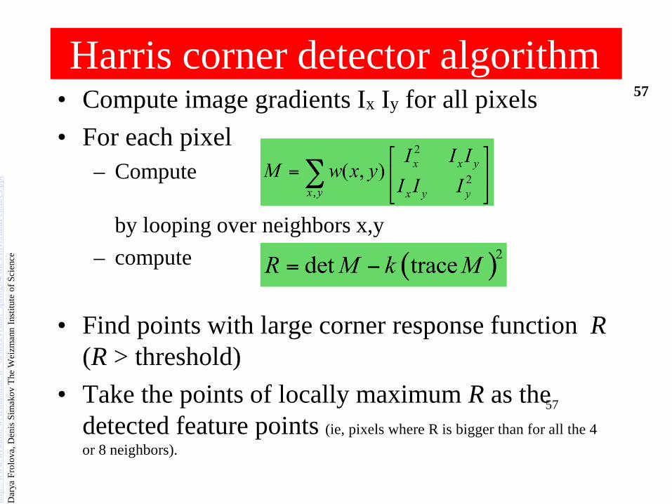
Harris corner detector algorithm• Compute image gradients Ix Iy for all pixels• For each pixel
– Compute
by looping over neighbors x,y– compute
• Find points with large corner response function R(R > threshold)
• Take the points of locally maximum R as the detected feature points (ie, pixels where R is bigger than for all the 4 or 8 neighbors).
57
http
://w
ww
.wis
dom
.wei
zman
n.ac
.il/~
deni
ss/v
isio
n_sp
ring0
4/fil
es/In
varia
ntFe
atur
es.p
ptD
arya
Fro
lova
, Den
is S
imak
ov T
he W
eizm
ann
Inst
itute
of S
cien
ce
57

Harris Detector - Example

Harris Detector - Example

Harris Detector - ExampleCompute corner response R

Harris Detector - ExampleFind points with large corner response: R>threshold

Harris Detector - ExampleTake only the points of local maxima of R

Harris Detector - ExampleMap corners on the original image

Harris Detector – Scale Parameters
• The Harris detector requires two scale parameters:
(i) a differentiation scale σD for smoothing prior to the computation of image derivatives,
&(ii) an integration scale σI for defining the size of the Gaussian window (i.e., integrating derivative responses). AW(x,y) AW(x,y,σI,σD)
• Typically, σI=γσD

Invariance to Geometric/Photometric Changes
• Is the Harris detector invariant to geometric and photometric changes?
• Geometric
– Rotation
– Scale
– Affine
• Photometric– Affine intensity change: I(x,y) → a I(x,y) + b

Harris Detector: Rotation Invariance
• Rotation
Ellipse rotates but its shape (i.e. eigenvalues) remains the same
Corner response R is invariant to image rotation

Harris Detector: Rotation Invariance (cont’d)

Harris Detector: Photometric Changes
• Affine intensity change Only derivatives are used => invariance to intensity shift I(x,y) → I (x,y) + b
Intensity scale: I(x,y) → a I(x,y)
R
x (image coordinate)
threshold
R
x (image coordinate)
Partially invariant to affine intensity change
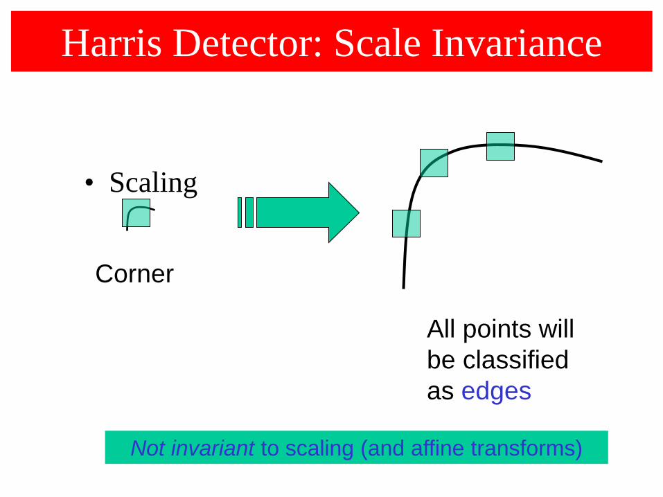
Harris Detector: Scale Invariance
• Scaling
All points will be classified as edges
Corner
Not invariant to scaling (and affine transforms)

Harris Detector: Disadvantages
• Sensitive to:– Scale change– Significant viewpoint change– Significant contrast change

How to handle scale changes?
• AW must be adapted to scale changes.
• If the scale change is known, we can adapt the Harris detector to the scale change (i.e., set properly σI ,σD).
• What if the scale change is unknown?

Multi-scale Harris Detector
scale
x
y
← Harris →
• Detects interest points at varying scales.R(AW) = det(AW(x,y,σI,σD)) – α trace2(AW(x,y,σI,σD))
σnσD= σnσI=γσD
σn=knσ

How to cope with transformations?
• Exhaustive search• Invariance• Robustness

Exhaustive search• Multi-scale approach
Slide from T. Tuytelaars ECCV 2006 tutorial

Exhaustive search• Multi-scale approach

Exhaustive search
• Multi-scale approach

Exhaustive search• Multi-scale approach

How to handle scale changes?
• Not a good idea!– There will be many points representing the same
structure, complicating matching! – Note that point locations shift as scale increases.
The size of the circle corresponds to the scale at which the point was detected

How to handle scale changes? (cont’d)
• How do we choose corresponding circles independently in each image?
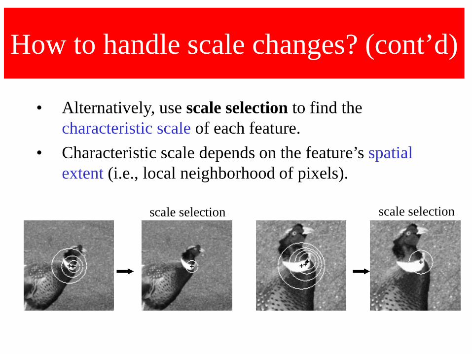
How to handle scale changes? (cont’d)
• Alternatively, use scale selection to find the characteristic scale of each feature.
• Characteristic scale depends on the feature’s spatial extent (i.e., local neighborhood of pixels).
scale selection scale selection

How to handle scale changes?
The size of the circles corresponds to the scale at which the point was selected.
• Only a subset of the points computed in scale space are selected!

Automatic Scale Selection• Design a function F(x,σn) which provides some local
measure. • Select points at which F(x,σn) is maximal over σn.
T. Lindeberg, "Feature detection with automatic scale selection" International Journal of Computer Vision, vol. 30, no. 2, pp 77-116, 1998.
max of F(x,σn)corresponds tocharacteristic scale!
σn
F(x,σn)

Invariance
• Extract patch from each image individually

Automatic scale selection• Solution:
– Design a function on the region, which is “scale invariant” (the same for corresponding regions, even if they are at different scales)
Example: average intensity. For corresponding regions (even of different sizes) it will be the same.
scale = 1/2
– For a point in one image, we can consider it as a function of region size (patch width)
f
region size
Image 1 f
region size
Image 2

Automatic scale selection• Common approach:
scale = 1/2f
region size
Image 1 f
region size
Image 2
Take a local maximum of this function
Observation: region size, for which the maximum is achieved, should be invariant to image scale.
s1 s2
Important: this scale invariant region size is found in each image independently!

Automatic Scale Selection• Function responses for increasing scale (scale signature)
88)),((
1σxIf
mii )),((1
σxIfmii ′

Automatic Scale Selection• Function responses for increasing scale (scale signature)
89)),((
1σxIf
mii )),((1
σxIfmii ′

Automatic Scale Selection• Function responses for increasing scale (scale signature)
90)),((
1σxIf
mii )),((1
σxIfmii ′

Automatic Scale Selection• Function responses for increasing scale (scale signature)
91)),((
1σxIf
mii )),((1
σxIfmii ′

Automatic Scale Selection• Function responses for increasing scale (scale signature)
92)),((
1σxIf
mii )),((1
σxIfmii ′

Automatic Scale Selection• Function responses for increasing scale (scale signature)
93)),((
1σxIf
mii )),((1
σ ′′xIfmii

Scale selection• Use the scale determined by detector to compute
descriptor in a normalized frame
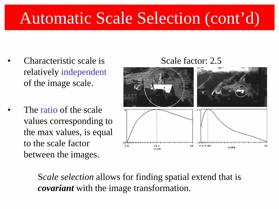
Automatic Scale Selection (cont’d)
• Characteristic scale is relatively independentof the image scale.
• The ratio of the scale values corresponding to the max values, is equal to the scale factor between the images.
Scale selection allows for finding spatial extend that is covariant with the image transformation.
Scale factor: 2.5

Automatic Scale Selection
• What local measures should we use? – Should be rotation invariant– Should have one stable sharp peak

How should we choose F(x,σn) ?
• Typically, F(x,σn) is defined using derivatives, e.g.:
• LoG yielded best results in a evaluation study; DoG was second best.
2 2 2
2
12
: ( ( , ) ( , ))
: | ( ( , ) ( , )) |
:| ( )* ( ) ( )* ( ) |
: det( ) ( )
x y
xx yy
n n
W W
Square gradient L x L x
LoG L x L xDoG I x G I x G
Harris function A trace A
σ σ σ
σ σ σ
σ σ
α−
+
+
−
−
C. Schmid, R. Mohr, and C. Bauckhage, "Evaluation of Interest Point Detectors", International Journal of Computer Vision, 37(2), pp. 151-172, 2000.

How should we choose F(x,σn) ?
• Let’s see how LoG responds at blobs …

Recall: Edge detection Using 1st derivative
gdxdf ∗
f
gdxd
Edge
Derivativeof Gaussian
Edge = maximumof derivative

Recall: Edge detection Using 2nd derivative
gdxdf 2
2
∗
f
gdxd
2
2
Edge
Second derivativeof Gaussian (Laplacian)
Edge = zero crossingof second derivative

From edges to blobs (i.e., small regions)
• Blob = superposition of two edges
Spatial selection: the magnitude of the Laplacian response will achieve a maximum (absolute value) at the center of he blob, provided the scale of the Laplacian is “matched” to the scale of the blob (e.g, spatial extent)
maximum
(blobs of different spatial extent)

How could we find the spatial extent of a blob using LoG?
• Idea: Find the characteristic scale of the blob by convolving it with Laplacian filters at several scales and looking for the maximum response.
• However, Laplacian response decays as scale increases:
Why does this happen?increasing σoriginal signal
(radius=8)

Scale normalization
• The response of a derivative of Gaussian filter to a perfect step edge decreases as σincreases
πσ 21

Scale normalization (cont’d)
• To keep response the same (scale-invariant), must multiply Gaussian derivative by σ
• Laplacian is the second Gaussian derivative, so it must be multiplied by σ2
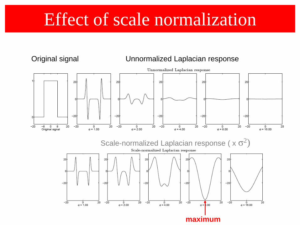
Effect of scale normalization
Scale-normalized Laplacian response ( x σ2)
Unnormalized Laplacian responseOriginal signal
maximum

What Is A Useful Signature Function?• Laplacian-of-Gaussian = “blob” detector
106

Scale selection: case of circle• At what scale does the Laplacian achieve a
maximum response for a binary circle of radius r?
r
imageLaplacian
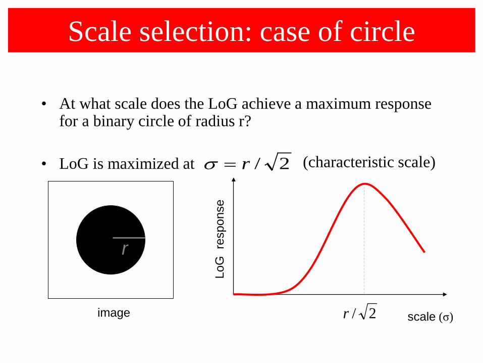
Scale selection: case of circle
• At what scale does the LoG achieve a maximum response for a binary circle of radius r?
• LoG is maximized at 2/r=σ
scale (σ)
r
2/rimage
LoG
res
pons
e
(characteristic scale)

Characteristic scale• We define the characteristic scale as the scale that
produces peak of Laplacian response
characteristic scaleT. Lindeberg (1998). "Feature detection with automatic scale selection."International Journal of Computer Vision 30 (2): pp 77--116. Source: Lana Lazebnik
2/r=σ

Scale-space blob detector: Example
Source: Lana Lazebnik

Scale-space blob detector: Example
Source: Lana Lazebnik

Scale-space blob detector: Example
Source: Lana Lazebnik

σn
Harris-Laplace Detector
scale
x
y
← Harris →
←Lo
G →
• Multi-scale Harris with scale selection.• Uses LoG maxima to find characteristic scale.

Harris-Laplace Detector (cont’d)
(1) Compute interest points at multiple scales using the Harris detector.
- Scales are chosen as follows: σn =knσ0 (σI =σn, σD =cσn)- At each scale, choose local maxima assuming 3 x 3 window
K. Mikolajczyk and C. Schmid (2001). “Indexing based on scale invariant interest points" Int Conference on Computer Vision, pp 525-531.
=
σn σn
σn
σnwhere

Harris-Laplace Detector (cont’d)
(2) Select points at which a local measure (i.e., normalized Laplacian) is maximal over scales.
K. Mikolajczyk and C. Schmid, “Indexing based on scale invariant interest points" Int Conference on Computer Vision, pp 525-531, 2001.
=
(s= σn)
σn σn-1 σn σn+1
σn
where:

Example
• Points detected at each scale using Harris-Laplace (images differ by a scale factor 1.92)– Few points detected in the same location but on different scales.– Many correspondences between levels for which scale ratio
corresponds to the real scale change between images.

Example
190 and 213 points detected in the left and right images, respectively (more than 2000 points would have been detected without scale selection)
(same viewpoint – change in focal length and orientation)
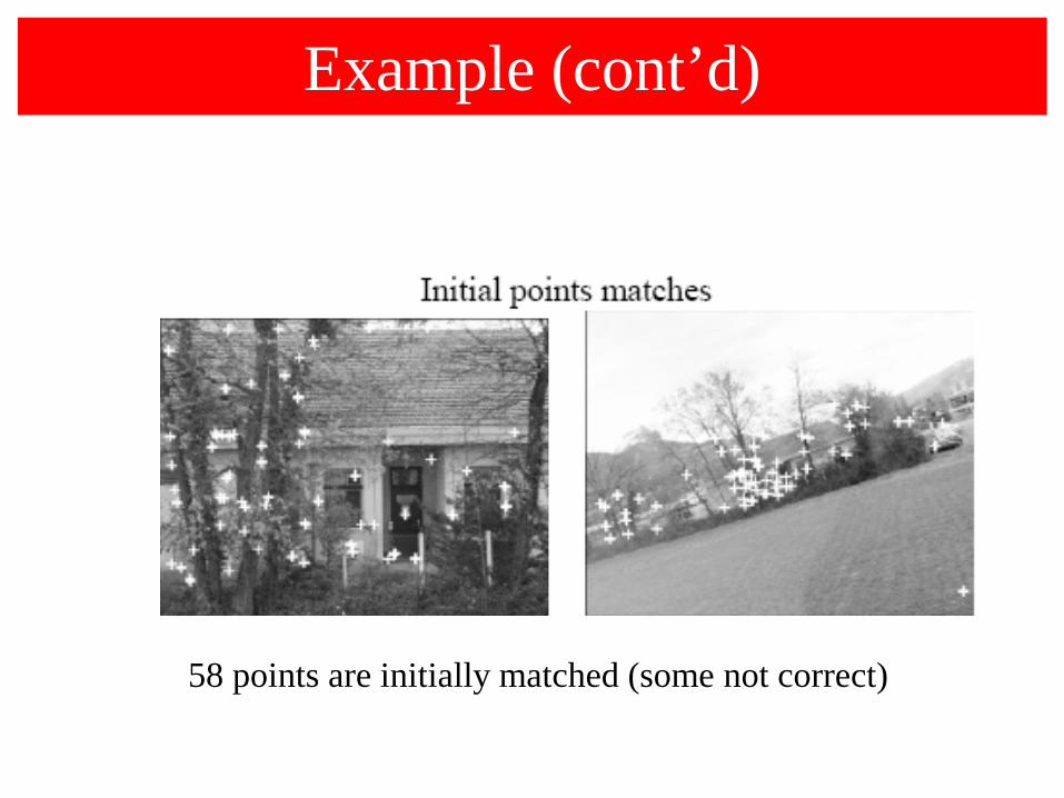
Example (cont’d)
58 points are initially matched (some not correct)

Example (cont’d)
• Reject inconsistent matches using RANSAC to compute the homography between images – left with 32 matches, all of which are correct.• The estimated scale factor is 4:9 and the estimated rotation angle is 19 degrees.

Harris-Laplace Detector (cont’d)
• Invariant to:– Scale– Rotation– Translation
• Robust to: – Illumination changes– Limited viewpoint changes
Repeatability

Efficient implementation using DoG
• LoG can be approximated by DoG:
• Note that DoG already incorporates the σ2 scale normalization.
2 2( , , ) ( , , ) ( 1)G x y k G x y k Gσ σ σ− ≈ − ∇

Efficient implementation using DoG (cont’d)
• Gaussian-blurred image
• The result of convolving an image with a difference-of Gaussian is given by:
),,(),,(),()),,(),,((),,(
σσσσσ
yxLkyxLyxIyxGkyxGyxD
−=∗−=
( , , ) ( , , ) ( , )L x y G x y I x yσ σ= ∗

Example
- =
),,(),,( σσ yxLkyxL −=

Efficient implementation using DoG (cont’d)
( ), , *G x y k Iσ( )( ) ( )( )
, ,
, , , , *
D x y
G x y k G x y I
σ
σ σ
=
−
( ), , *G x y Iσ
( )2, , *G x y k Iσ
David G. Lowe. "Distinctive image features from scale-invariant keypoints.” IJCV 60 (2), pp. 91-110, 2004.
σn =knσ
DoG
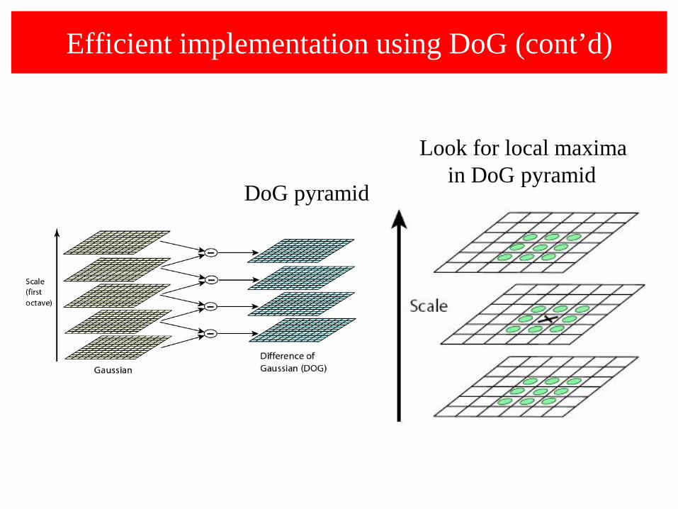
Efficient implementation using DoG (cont’d)
Look for local maximain DoG pyramid
DoG pyramid
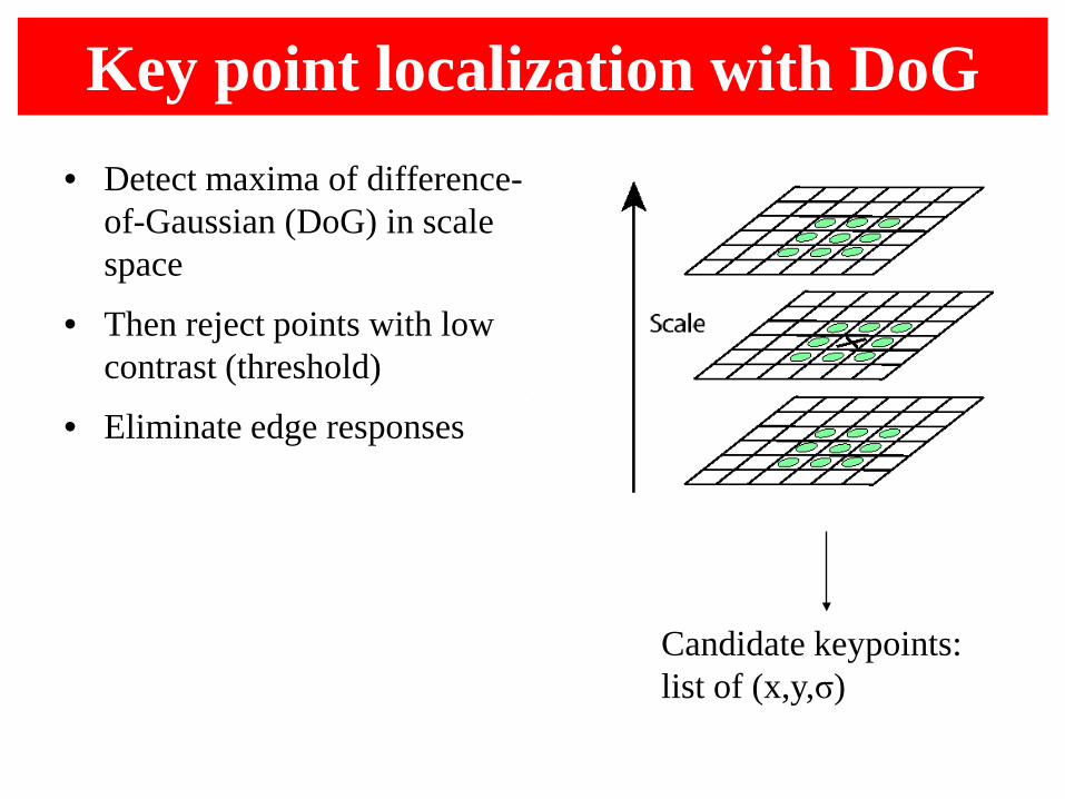
Key point localization with DoG• Detect maxima of difference-
of-Gaussian (DoG) in scale space
• Then reject points with low contrast (threshold)
• Eliminate edge responsesBlur
Resample
Subtract
Candidate keypoints: list of (x,y,σ)

Example of keypoint detection
(a) 233x189 image(b) 832 DOG extrema(c) 729 left after peak
value threshold(d) 536 left after testing
ratio of principlecurvatures (removing
edge responses)
Review• Homography and Ransac
• ReProjection method from an image to another
• Robust fitting of the Mapping
• Interest Points• Corner Detection: Harris Detector
• Scaling Issues• Harris-Laplace Detector
#128