Lecture 9: LinearRegression

Goals

• Linear regression in R

• Estimating parameters and hypothesis testingwith linear models

• Develop basic concepts of linear regression froma probabilistic framework

Regression

• Technique used for the modeling and analysis ofnumerical data

• Exploits the relationship between two or morevariables so that we can gain information about one ofthem through knowing values of the other

• Regression can be used for prediction, estimation,hypothesis testing, and modeling causal relationships

Regression Lingo

Y = X1 + X2 + X3

Dependent Variable

Outcome Variable

Response Variable

Independent Variable

Predictor Variable

Explanatory Variable

Why Linear Regression?

• Suppose we want to model the dependent variable Y in termsof three predictors, X1, X2, X3

Y = f(X1, X2, X3)

• Typically will not have enough data to try and directlyestimate f

• Therefore, we usually have to assume that it has somerestricted form, such as linear

Y = X1 + X2 + X3

Linear Regression is a Probabilistic Model

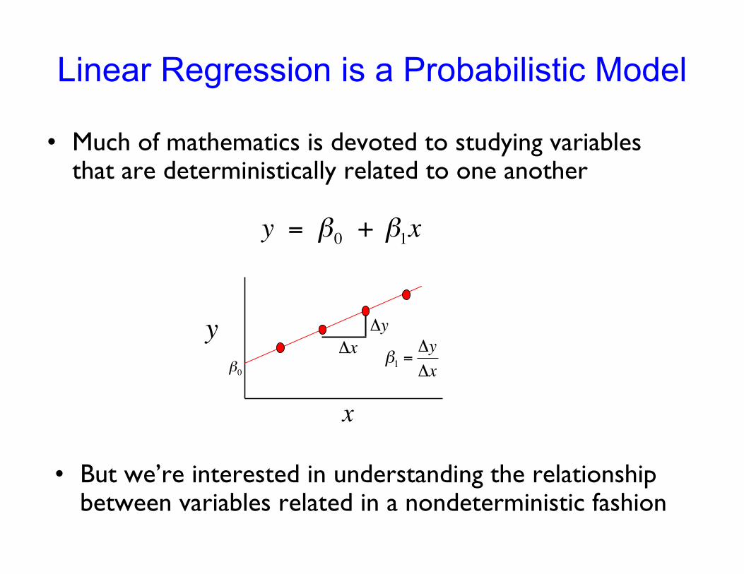
• Much of mathematics is devoted to studying variablesthat are deterministically related to one another

!

y = "0 + "

1x

!

"0

!

y

!

x

!

"1

=#y

#x

!

"y

!

"x

• But we’re interested in understanding the relationshipbetween variables related in a nondeterministic fashion

A Linear Probabilistic Model

!

"0

!

y

!

x

!

y = "0 + "

1x + #

• Definition: There exists parameters , , and , such that forany fixed value of the independent variable x, the dependentvariable is related to x through the model equation

!

"0

!

"1

!

" 2

•

!

" is a rv assumed to be N(0, # 2)

!

y = "0 + "

1x

True Regression Line

!

"1

!

"2

!

"3

Implications

• The expected value of Y is a linear function of X, but for fixedx, the variable Y differs from its expected value by a randomamount

• Formally, let x* denote a particular value of the independentvariable x, then our linear probabilistic model says:

!

E(Y | x*) = µY|x* = mean value of Y when x is x *

!

V (Y | x*) = "Y|x*

2 = variance of Y when x is x *

Graphical Interpretation

!

y = "0 + "

1x

!

"0 + "

1x

1!

"0 + "

1x

2

!

x1

!

x2

!

y

!

x

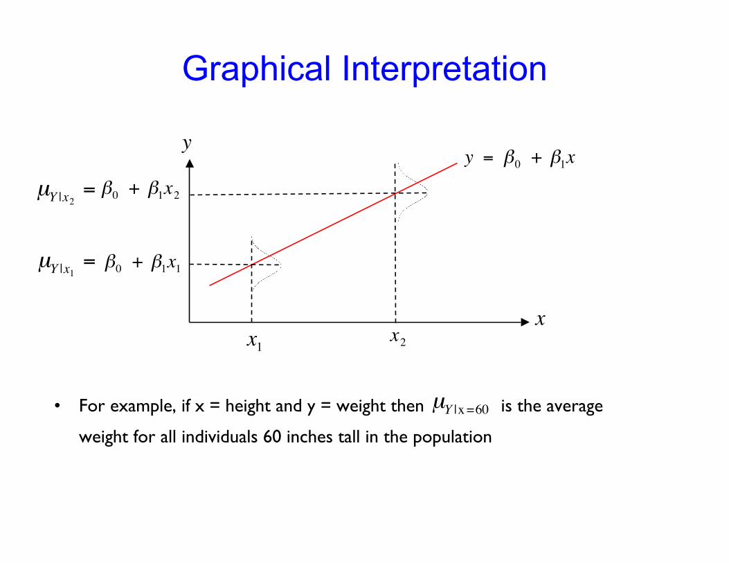
• For example, if x = height and y = weight then is the average

weight for all individuals 60 inches tall in the population

!

µY |x

1

=

!

µY |x

2

=

!

µY |x =60

One More ExampleSuppose the relationship between the independent variable height

(x) and dependent variable weight (y) is described by a simplelinear regression model with true regression line

y = 7.5 + 0.5x and

• Q2: If x = 20 what is the expected value of Y?

!

µY |x =20 = 7.5 + 0.5(20) = 17.5

• Q3: If x = 20 what is P(Y > 22)?

• Q1: What is the interpretation of = 0.5?

!

"1

The expected change in height associated with a 1-unit increasein weight !

" = 3

!

P(Y > 22 | x = 20) = P22 -17.5

3

"

# $

%

& ' =1()(1.5) = 0.067

Estimating Model Parameters

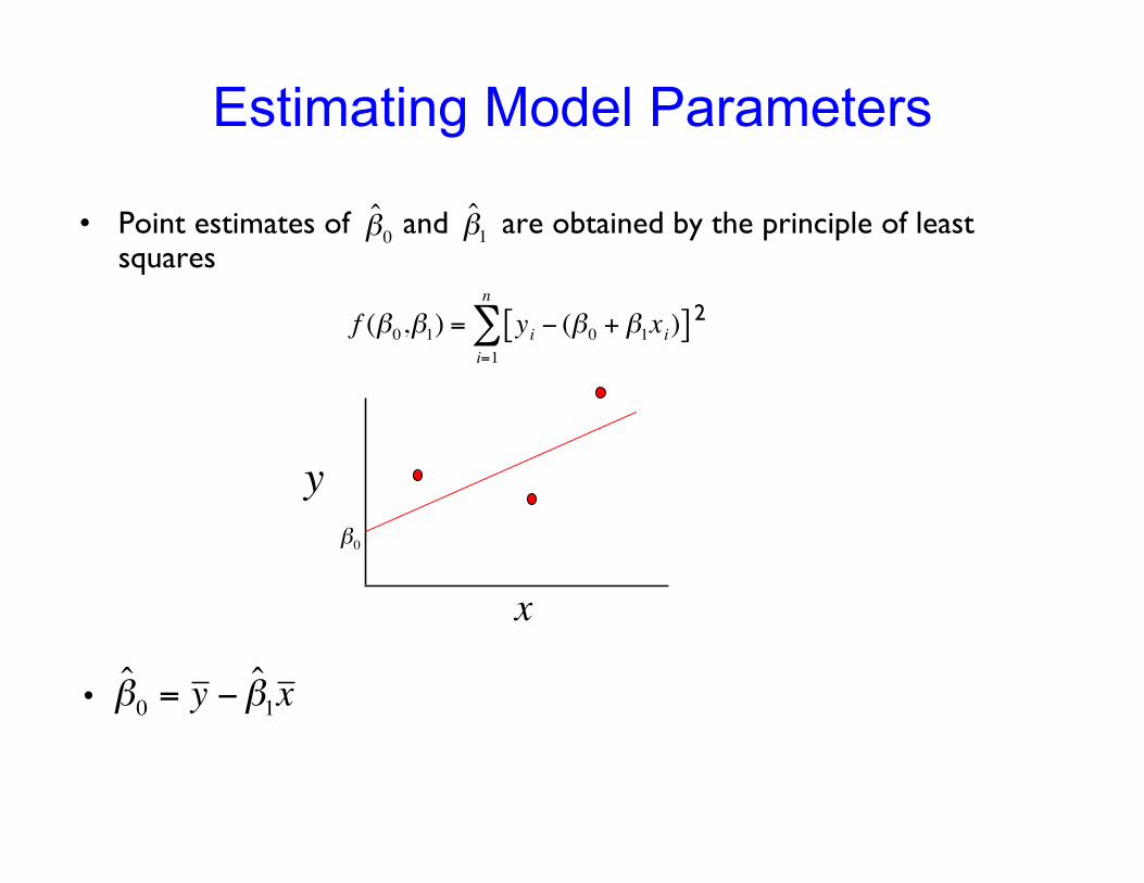
• Point estimates of and are obtained by the principle of leastsquares

!

ˆ " 0

!

ˆ " 1

!

f ("0,"1) = yi # ("0 + "

1xi)[ ]

i=1

n

$ 2

!

"0

!

y

!

x

•

!

ˆ " 0

= y # ˆ " 1x

Predicted and Residual Values

• Predicted, or fitted, values are values of y predicted by the least-squares regression line obtained by plugging in x1,x2,…,xn into theestimated regression line

!

ˆ y 1

= ˆ " 0# ˆ "

1x

1

!

ˆ y 2

= ˆ " 0# ˆ "

1x

2

• Residuals are the deviations of observed and predicted values

!

e1

= y1" ˆ y

1

e2

= y2" ˆ y

2

!

y

!

x!

e1

!

e2

!

e3

!

ˆ y 1

!

y1

Residuals Are Useful!

!

SSE = (ei

i=1

n

" )2

= (yi

i=1

n

" # ˆ y i)2

• They allow us to calculate the error sum of squares (SSE):

• Which in turn allows us to estimate :

!

" 2

!

ˆ " 2 =SSE

n # 2

• As well as an important statistic referred to as the coefficient ofdetermination:

!

r2

=1"SSE

SST

!

SST = (yi " y )2

i=1

n

#

Multiple Linear Regression

• Extension of the simple linear regression model to two ormore independent variables

!

y = "0 + "

1x

1 + "

2x

2+ ...+ "n xn + #

• Partial Regression Coefficients: βi ≡ effect on thedependent variable when increasing the ith independentvariable by 1 unit, holding all other predictorsconstant

Expression = Baseline + Age + Tissue + Sex + Error

Categorical Independent Variables

• Qualitative variables are easily incorporated in regressionframework through dummy variables

• Simple example: sex can be coded as 0/1

• What if my categorical variable contains three levels:

xi =

0 if AA1 if AG2 if GG

Categorical Independent Variables

• Previous coding would result in colinearity

• Solution is to set up a series of dummy variable. In generalfor k levels you need k-1 dummy variables

x1 =1 if AA0 otherwise

x2 =1 if AG0 otherwise

AA

AG

GG

x1 x2

110

000

Hypothesis Testing: Model Utility Test (orOmnibus Test)

• The first thing we want to know after fitting a model is whetherany of the independent variables (X’s) are significantly related tothe dependent variable (Y):

!

H0 : "1 = "2 = ... = "k = 0

HA : At least one "1 # 0

f =R

2

(1$ R2)

•k

n $ (k +1)

!

Rejection Region : F",k,n#(k+1)

Equivalent ANOVA Formulation of Omnibus Test

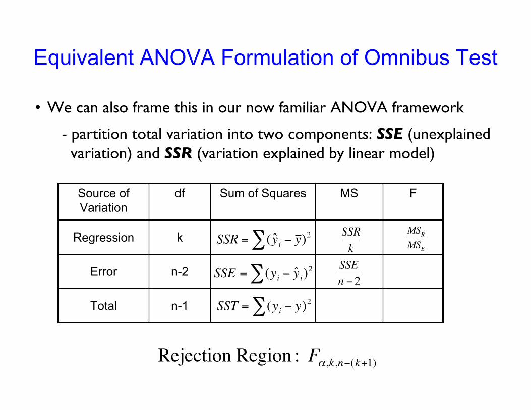
• We can also frame this in our now familiar ANOVA framework

- partition total variation into two components: SSE (unexplainedvariation) and SSR (variation explained by linear model)

Equivalent ANOVA Formulation of Omnibus Test

• We can also frame this in our now familiar ANOVA framework

!

Rejection Region : F",k,n#(k+1)

- partition total variation into two components: SSE (unexplainedvariation) and SSR (variation explained by linear model)

n-1Total

n-2Error

kRegression

FMSSum of SquaresdfSource ofVariation

!

SSR

k

!

SSE

n " 2!

MSR

MSE

!

SSR = ( ˆ y i " y )2#

!

SSE = (yi " ˆ y i)2#

!

SST = (yi " y )2#

F Test For Subsets of Independent Variables

• A powerful tool in multiple regression analyses is the ability tocompare two models

• For instance say we want to compare:

!

Full Model : y = "0 + "

1x

1 + "

2x

2+ "

3x

3+ "

4x

4+ #

!

Reduced Model : y = "0 + "

1x

1 + "

2x

2+ #

!

f =(SSER " SSEF ) /(k " l)

SSEF /([n " (k +1)]

• Again, another example of ANOVA:

SSER = error sum of squares forreduced model with predictors

!

l

SSEF = error sum of squares forfull model with k predictors

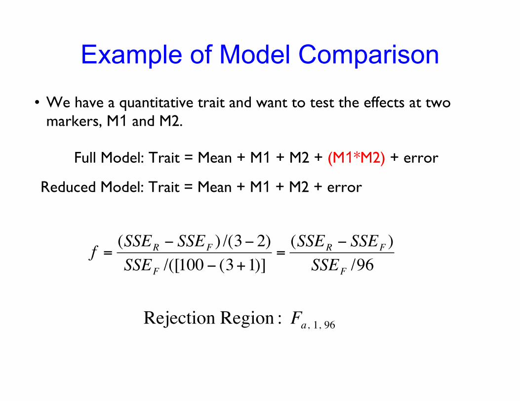
Example of Model Comparison

• We have a quantitative trait and want to test the effects at twomarkers, M1 and M2.

!

f =(SSER " SSEF ) /(3" 2)

SSEF /([100 " (3+1)]=(SSER " SSEF )

SSEF /96

Full Model: Trait = Mean + M1 + M2 + (M1*M2) + error

Reduced Model: Trait = Mean + M1 + M2 + error

!

Rejection Region : Fa, 1, 96

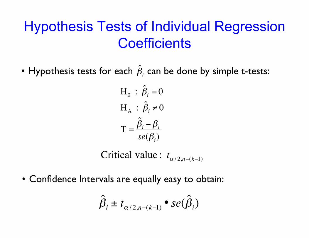
Hypothesis Tests of Individual RegressionCoefficients

• Hypothesis tests for each can be done by simple t-tests:

!

ˆ " i

!

H0 : ˆ "

i= 0

HA : ˆ "

i# 0

T =ˆ " i$"

i

se("i)

• Confidence Intervals are equally easy to obtain:

!

ˆ " i± t# / 2,n$(k$1)

• se( ˆ " i)!

Critical value : t" / 2,n#(k#1)

Checking Assumptions• Critically important to examine data and check assumptions

underlying the regression model

Outliers Normality Constant variance Independence among residuals

• Standard diagnostic plots include: scatter plots of y versus xi (outliers) qq plot of residuals (normality) residuals versus fitted values (independence, constant variance) residuals versus xi (outliers, constant variance)

• We’ll explore diagnostic plots in more detail in R

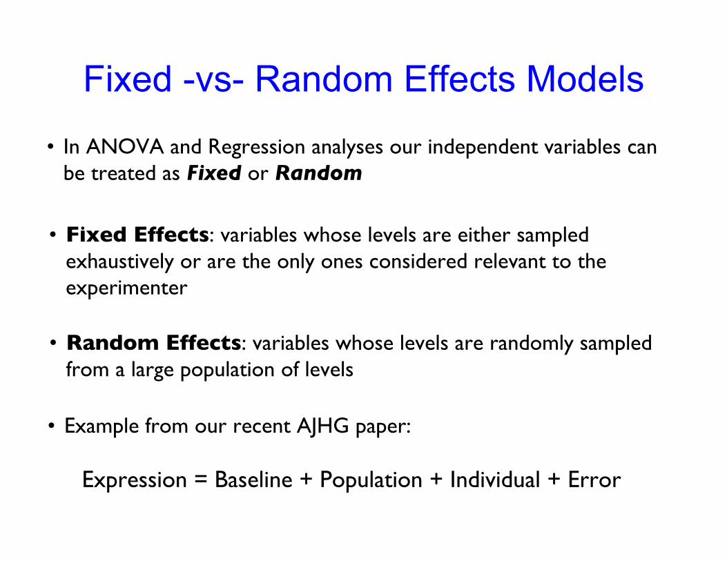
Fixed -vs- Random Effects Models

• In ANOVA and Regression analyses our independent variables canbe treated as Fixed or Random

• Fixed Effects: variables whose levels are either sampledexhaustively or are the only ones considered relevant to theexperimenter

• Random Effects: variables whose levels are randomly sampledfrom a large population of levels

Expression = Baseline + Population + Individual + Error

• Example from our recent AJHG paper: