lecture 9 mgmt 7730 - © 2011 houman younessi oligopoly an oligopoly is a market structure with a...

Lecture 9

MGMT 7730 - © 2011 Houman Younessi

Oligopoly

An oligopoly is a market structure with a small number of firms together controlling the market.

Lecture 9


Oligopoly

There is no single model of oligopolistic behavior. In general there is a spectrum bounded by:

A Collusive Model A Contestable Market Model

We shall discuss these two general models and various forms within them

Lecture 9


Contestable Market Model

In it’s extreme, this is a market structure where the firms in an oligopoly compete against one-another as if there was no oligopoly; that is they compete freely in the market.

In general however there are degrees of this market structure. Oligopolies engaged in a contestable market model usually compete on the basis of price or market share but they use specific characteristics emerging from the fact that they are oligopolies to their benefit.

We will examine some of these.

Lecture 9


Contesting the Market Based on Price

This is the situation of price competition where firms in an oligopoly compete against one-another based on price.

Consider the simple situation – without loss of generality – of a duopoly (a market with only two operators in it).

Further assume that there is a simultaneous game established between them. That is, they make business decisions – set prices and quantities – independently of each other. (Remember this is a limiting case)

Furthermore the two firms produce identical products and have identical cost functions

Lecture 9


Let us assume that the cost function for either firms is:

25.04500 XX QQTC

The market demand seen by both firms:

BA QQQP 100100

The marginal cost for a firm would be:

XXXX QdQdTCMC 4/

Lecture 9


In a pure competitive environment, both firms will be willing – would eventually have to – bring down their prices to the marginal cost (but not lower than it)

For both firm A and B:

BA

AABA

QQ

MCQQQP

5.048

4100

AB

BBBA

QQ

MCQQQP

5.048

4100

Solving for one of the Q’s

32

)5.048(5.048

B

BB

Q

QQ similarly 32AQ

And therefore 64 AB QQQ

Lecture 9


Substituting in the demand equation:

36$64100100 QP

Total revenue: 1152$3236$

And a total cost of: 1140$)32(5.0)32(4500 2

Leaving a profit of: 12$1140$1152$

We will contrast this case with that of collusive behavior later in the lecture

Lecture 9


Price Leadership

In some oligopolies, one firm sets the price and others follow. The firm that sets the price is called a:

Price Leader

How should the price leader set the price and output levels?

Under this model, the price leader sets the price but allows all other smaller operators to sell at that price. Whatever amount the small firms DONOT supply at the price provided, will be picked up by the price leader.

Lecture 9


It is important to note:

1. The price leader controls the market. If a price follower tries to sell below the set price, the price leader will move in and take up that market share

2. The price follower cannot of course sell at a price higher than the one set by the market leader as there will be no incentive for the consumer to by at a higher price

As such, prices stabilize at the price set by the price leader

Lecture 9


Setting a price – as a price leader:

1. As each small firm will take the price as given, they would produce output at the quantity such that their price equals their marginal cost.

2. As such a supply curve for each and therefore for all (as a horizontal sum of all their marginal costs) small suppliers may be obtained.

3. The demand curve of the dominant firm can be derived by subtracting the amount supplied by the small firms from the total amount demanded (note that demand varies with price. That is demand varies if different prices are set by the dominant firm and followed by the small firms).

Lecture 9


4. Thus the demand curve for the dominant firm D can be obtained as the horizontal difference at each price between the market demand curve and the supply curve of the dominated firms.

5. The dominant curve knows its marginal cost (MC). By determining the demand curve as above, it can set the price and quantity at a point where MC intersects its demand curve and as such maximize profits.

6. Of course, this would not necessarily be a point of maximum profit (usually it is not) for the smaller operators collectively or individually.

Lecture 9


Example: Home Depot

A simplified demand curve for home improvement supplies in a given town is:

PQ 5100 The demand curve for the Mom and Pop home improvement store(s) in the same region is:

PQ PM 10&

Home depot’s marginal cost is:

HDQMC 2

Lecture 9


To derive the demand for Home Depot’s products:

PPPQQQ PMHD 690)10()5100(&

Home Depot’s total revenue is of course:

261

61 15)15( HDHDHDHDHD QQQQPQTR

The price is therefore:

HDHD

HD

QQP

PQ

61

690

61 15

690

Lecture 9


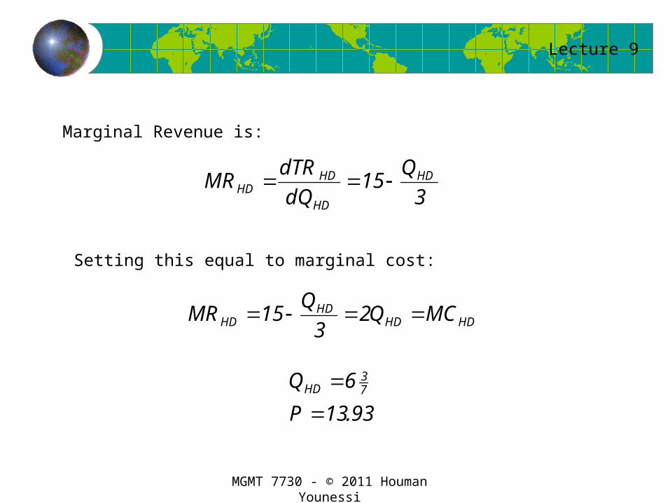
Marginal Revenue is:

315 HD

HD

HDHD

Q

dQ

dTRMR

Setting this equal to marginal cost:

HDHDHD

HD MCQQ

MR 23

15

93.13

6 73

P

QHD

Lecture 9


Collusion and Cartels

Conditions in oligopolistic industries often favor collusion amongst the organizations forming the oligopoly:

Numbers are small, and

Firms are aware of their interdependence

Collusion has its advantages:

Increased profit

Decreased uncertainty

Better opportunity to prevent entry of new players

Lecture 9


But collusion also brings forth some issues and problems:

Unilateral breaking of collusion by one or a few firms may lead to substantial losses for those who have not broken collusion

They are often forbidden by law or by cultural norms

Even when no intent is there to break collusion, it is expensive to maintain a collusive agreement

Products have to be homogeneous

If collusion is in the open, it is often called a cartel and the action is called price or supply regulation

Most national laws prohibit formation of cartels but they do exist as international entities. Examples include OPEC and IATA (International Air Transport Association)

Lecture 9


Breakdown of Collusion

It is not surprising that collusive arrangements tend to break down.

What happens however is that they usually break down, the market re-organizes, new collusions are formed only to break down again……

QC QR

ATC

MC

MR

PC

PR

BC

BR Demand

PC is price set by cartel

PR is price set by rouge seller

BC is the base cost @cartel

BR is base cost rouge seller

Lecture 9


Given that demand in oligopolies is often extremely elastic with respect to price, it can be seen that if a seller cheats or even has a secret “side-arrangement” at a lower price, it can increase profits significantly.

From game theory we know that if we engage in a one-shot or a limited horizon game, it pays to cheat if the consequences of cheating are bearable

For a cartel participant, if the intent is to stay in the cartel, then cheating is not an option. However, the cartel participants know that the other participants are likely to break the cartel if opportunity arises and therefore the cartel will break anyway, so why not let it be them who breaks it and at least reaps the benefit?

Lecture 9


On the other hand, they know that the cartel’s survival is to their collective advantage and if there is no cheating, then it is best to stay in the cartel.

They also know that if caught cheating, they may be punished.

In final analysis, they would break cartel if they are confident that their cheating will not be discovered too early (see the mathematics of cheating in lecture 6) or that if discovered, the punishment will not be sufficiently harsh.

The largest and most powerful players in the cartel would want the cartel to survive, why?

They will do whatever it takes to keep it together…..

Lecture 9


They (and other cartel members) would expend effort to make it impossible to cheat. This is done two ways:

• Regulation and watchdogs

• Threat of severe punishment

Regulation and use of watchdogs are instituted to make it systemically impossible to cheat

Threat of punishment is there to make it psychologically and economically unprofitable to cheat

Lecture 9


When regulations and watchdogs are inadequate (often) or are corrupted, the first method fails

Use of punishment is an interesting case:

If punishment is harsh enough – it will work and will keep the cartel together (e.g. Colombian drug cartels) but only for a limited period. Often the “enforcer” becomes too powerful and triggers a rebellion that causes the cartel to collapse

If they are not harsh enough– the cartel will fall apart

Reality is though that as most “legal” cartels are international entities, punishment must be administered internationally and unless the commodity in question is of extraordinary value (e.g. oil) national governments will not unite to form an international “punishment” force. As such punishment often does not work over international cartels.

Lecture 9


Collusive Pricing

Let us review the case of contesting the market based on price:

Total revenue: 1152$3236$

And a total cost of: 1140$)32(5.0)32(4500 2

Leaving a profit of: 12$1140$1152$

We had:25.04500 XX QQTC

XXXX QdQdTCMC 4/

Lecture 9


Now let us examine the case of a duopoly where there is collusion:

The cartel’s marginal cost will be the horizontal sum of the two marginal cost curves, in our case:

MCQ

MCQ

MCQ

AB

BA

28

4

4

The cartel will set its marginal revenue equal to its marginal cost (as it will wish to act monopolistically)

2100)100( QQQQPQTR

Lecture 9


The marginal revenue will be:

QdQ

dTRMR 2100

Setting marginal cost and marginal revenue equal:

4.38

5.042100

Q

MCQQMR

Substituting in the cartel demand curve, we get a price of $100-$38.4= $61.6

The cartel’s total revenue is $61.6 x 38.4 = $2,365.44

As each firm produces the same amount (38.4 / 2 = 19.2), they both have the same marginal cost (4+19.2 = $23.2)

Lecture 9


Also the firms likewise will split the total revenue:

72.182,1$2/44.2365$ PQTR

Each firm has a total cost of:

12.761$)2.19(5.0)2.19(4500 2 TC

Each firm therefore makes a profit of:

60.421$12.761$72.182,1$ TCTR

This is more than 35 times the profit of $12 if they were to compete !!!

Lecture 9


Capacity (Quantity) Competition

Given the difficulty of maintaining a collusive arrangement and the general social and legal undesirability of cartel arrangements, how can firms avoid the lose-lose situation of direct competition and approach the win-win of a cartel arrangement without collusion?

The answer is to try to reach Nash Equilibrium.

This can be done by competing on quantity (production capacity)

Lecture 9


Reaching a Nash Equilibrium – Cournot Solution

Let us first make certain assumptions:

1. The firms move simultaneously

2. They have the same view of the market (e.g. they see the same demand curve)

3. Know each other’s cost functions

4. They optimize their quantity decision assuming the other firm’s quantity decision is given

These are all reasonable assumptions.

Lecture 9


Using the details from the previous example, we now solve for maximizing profit when the competitor’s profit is maximized (Nash Equilibrium)

Let us be firm A:

We maximize profit when our total revenue PQA exceed our total cost maximally.

BAAAABAA QQQQQQQPQTR 2100)100(

Our marginal revenue is:

BAA

AA QQ

Q

TRMR

2100

Lecture 9


To maximize profit, we set MC=MR

BA

ABAA

QQ

QQQMR

3132

42100

This is called the reaction function of firm A (us). It tells us the profit maximizing amount to produce, given the output of our competitor.

Because firm B has the same cost function, and both firms face the same market demand curve, firm B’s reaction function is similarly:

AB

BABB

QQ

QQQMR

3132

42100

Note that this does not need to necessarily be the case and reaction functions may differ. The analysis will however remain the same

Lecture 9


Solving the two equations for the two unknown quantities QA and QB will give the respective production quantities for each firm.

It turns out that QA=QB=24 and as such Q=QA+QB=48

As P=100-Q, then price is P=100-48=$52

So each firm makes a total revenue of $1248 (52x24) and each firm’s total cost is $884 and each firm makes a profit of $364

Whilst this is not quite the profit that a collusive arrangement would yield, it is still over 30 times better than the pure competition price

Lecture 9


First Mover Advantage

Now, let us consider the situation where one firm gets to move (set quantity and price) before the other firm.

This can be done right (when the price set is such that it maximizes the other party’s profit having now had to go second) or wrong (when the price set is not optimal for the adversary).

If set right, our firm can rest assured that the adversary will not come into the market with a different price.

Using the information from our running example:

AAABA QQQQQP 32

31 68)32(100)100(

Let us say that we (firm A) move first.

Does the early bird get the worm?

Lecture 9


Our firm’s total revenue will be:

23268 AAA QQPQTR

Our marginal revenue is:

AA

AA Q

Q

TRMR 3

468

So we will set our marginal revenue equal to our marginal cost:

43.27

468 34

A

AAAA

Q

MCQQMR

Lecture 9


Substituting into firm B’s reaction function yields

86.2243.2732 31 BQ

Therefore Q=22.86+27.43=50.29

Substituting into the demand curve function gives the price $49.71.

Our revenue is $1,363.59 and firm B’s revenue is $1,136.33

Respective profits are (you calculate the costs): $377.71 and $283.67

It pays to be first – Early bird gets the worm

lecture 9 mgmt 7730 - © 2011 houman younessi oligopoly an oligopoly is a market structure with a...

Documents

set price

price set

price follower

price higher

higher price

basis of price

market leader

lecture slide