lecture atmospheric physics 2003 - …vijay/lectures/...physics_03.pdf · atmospheric physics - 3 -...
TRANSCRIPT

Lecture Atmospheric Physics University of Bremen
Master of Environmental Physics WS 2003 / 2004
Andreas Richter
room U2090, tel. 4474 [email protected]
Tutorial: Oluyemi Afe
room U2080, tel. 7421 [email protected]
Contents: 1. Survey of the Atmosphere 2. Radiation in the Atmosphere 3. Climate Change 4. Atmospheric Thermodynamics and the
role of Water Vapour 5. Introduction to Dynamics of the Atmosphere
Atmospheric Physics - 2 - University of Bremen, WS 2003 / 2004
Disclaimer This file contains the lecture notes for the Atmospheric Physics lecture given at the University Bremen during the winter term 2003 / 2004. This is not a book, and much of the information given in the lecture is missing. Also, many figures and explanations were taken from books, articles and web pages without proper reference. In particular, many parts are based on the script by K. Künzi and S. Bühler. The contents of this file may therefore used only for educational purposes. There probably are errors, omissions, inconsistencies and confusing explanations in these lecture notes. If you find any of these, please send an email to [email protected]

Atmospheric Physics - 3 - University of Bremen, WS 2003 / 2004
The Rules of the Game: Lectures: • 13 lectures, every Wednesday • one “rapporteur” gives brief summary from last
lecture
Exercises: • 10 exercises • will be distributed in the lecture • will have to be submitted on the next Tuesday
(6 days to work on it...) • no copies, joined solutions, cryptic notes
please! • will be returned and discussed on the next day
in the tutorial after the lecture • credits: 10 x 10 = 100
Exam: • prerequisite to take part in the exam:
o at least 75 credits from exercises o acted at least once as rapporteur
• 2 hours written exam in the first or second week after the end of lectures

Atmospheric Physics - 4 - University of Bremen, WS 2003 / 2004
Literature for the Lecture English Books: Houghton, J.T., The physics of atmospheres, Cambridge University Press, 1977, ISBN 0 521 29656 0 Wallace, John M. and Peter V. Hobbs, Atmospheric Science, Academic Press, 1977, ISBN 0-12-732950-1 Deutsche Bücher: Roedel, Walter, Physik unserer Umwelt, Die Atmosphäre, Springer Verlag, 1992, ISBN 3-540-54285-X Script: Environmental Physics I, WS 2002/2003, Klaus Künzi and Stefan Bühler, Institute of Environmental Physics, University of Bremen, Bremen; Germany

Atmospheric Physics - 5 - University of Bremen, WS 2003 / 2004
Schematic Overview
Cosmic Radiation Sun Extraterrestrial Effects
Radiation Absorption and
Emission Green House
Chemistry Photolysis
Trace Species (special course)
Water Thermodynamics
Clouds Precipitation
Stability
Dynamics
Earth surface: Land, Orography, Albedo, Ocean and
Ocean Dynamics
Atmospheric Physics - 6 - University of Bremen, WS 2003 / 2004
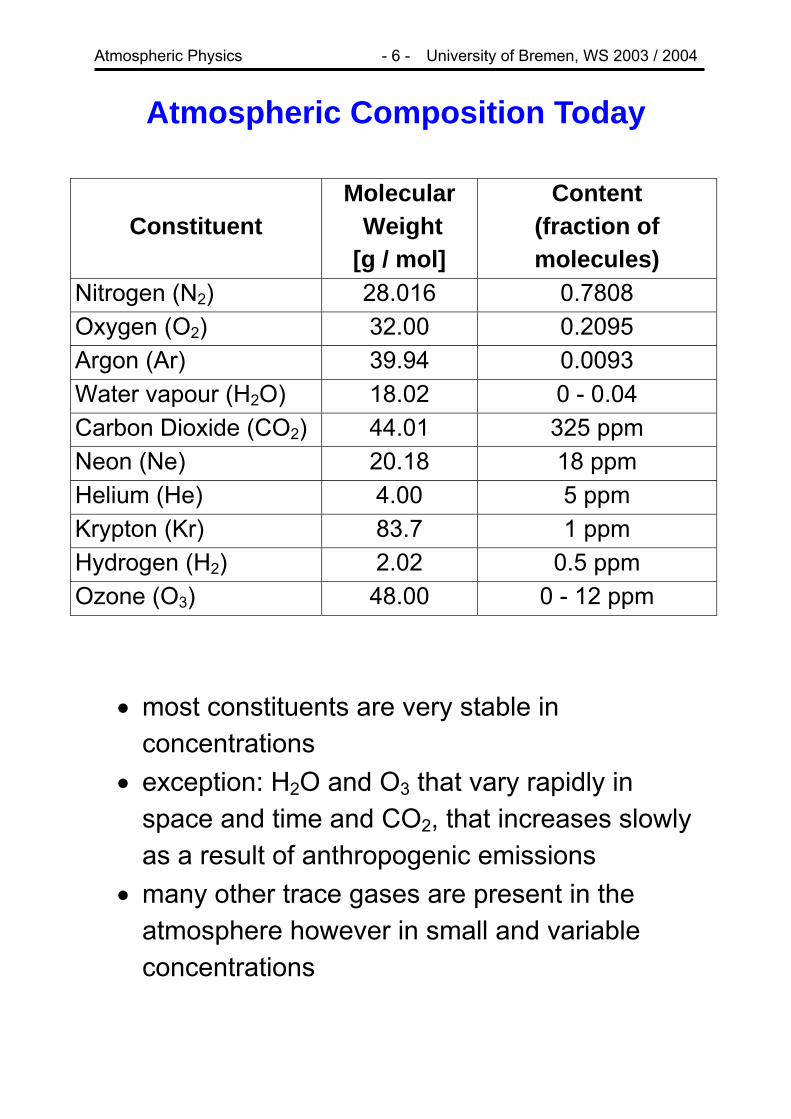
Atmospheric Composition Today
Constituent Molecular Weight [g / mol]
Content (fraction of molecules)
Nitrogen (N2) 28.016 0.7808 Oxygen (O2) 32.00 0.2095 Argon (Ar) 39.94 0.0093 Water vapour (H2O) 18.02 0 - 0.04 Carbon Dioxide (CO2) 44.01 325 ppm Neon (Ne) 20.18 18 ppm Helium (He) 4.00 5 ppm Krypton (Kr) 83.7 1 ppm Hydrogen (H2) 2.02 0.5 ppm Ozone (O3) 48.00 0 - 12 ppm
• most constituents are very stable in
concentrations • exception: H2O and O3 that vary rapidly in
space and time and CO2, that increases slowly as a result of anthropogenic emissions
• many other trace gases are present in the atmosphere however in small and variable concentrations

Atmospheric Physics - 7 - University of Bremen, WS 2003 / 2004
Planetary Atmospheres
Planet
Gravitation
(relative)
Temperature at Surface
[K]
SurfacePressur
e [103 hPa]
Composition
Venus
0.91 700 100 CO2 > 90%
Earth 1 290 1 N2
(~ 78 %) O2
(~ 21 %)
Mars 0.38 210 0.01 CO2
(> 80 %) • Earth’s atmosphere is unique in pressure,
temperature and atmospheric composition
Atmospheric Physics - 8 - University of Bremen, WS 2003 / 2004
Origin of the Atmosphere • at the time of formation (4.5 x 10⁹ years ago),
earth had no or little atmosphere • the atmosphere was formed from volatile
emissions from the interior of the earth (volcanic activity)
• volcanic emissions are roughly 85% H2O, 10% CO2, and a few per cent sulphur compounds
Questions: • where is the CO2?
o in carbonates in the earth’s crust • where is the H2O?
o deep ocean leakage o photodissociation?
• where is the O2 coming from? o photodissociation 2H2O + hν → 2H2 + O2 o photosynthesis H2O + CO2 → CH2O + O2
• where is the N2 coming from? • where are the noble gases coming from?
o radioactive decay

Atmospheric Physics - 9 - University of Bremen, WS 2003 / 2004
The Carbon Budget • in photosynthesis, carbon is incorporated into
organic compounds • a small part of this organic matter is not
oxidized, but fossilized in shales or fossil fuels • 90% of the O2 produced by photosynthesis is
stored in the earth’s crust in oxides such as FeO3 or carbonate compounds such as CaCO3, Fe2O3, or MgCO3
• the carbonates are the main sink of atmospheric CO2
Substance Fraction [%]
Rocks 71 Shales 29 Ocean, dissolved CO2 0.1 Oil, gas, coal 0.03 Atmosphere (CO2) 0.003 Biosphere 7x10⁻⁵

Atmospheric Physics - 10 - University of Bremen, WS 2003 / 2004
Inputs / Outputs to the Atmosphere
• Input from volcanic activity • Input from meteorites • Exchange with Biosphere • Exchange with Hydrosphere • Loss to outer space and earth

Atmospheric Physics - 11 - University of Bremen, WS 2003 / 2004
Impact of Biosphere
• The Earth’s atmosphere is far away from the
equilibrium expected for a planet without life. • The disequilibrium is sustained by permanent
emissions and adsorptions of species by the biosphere.
• Many feedback mechanisms are known through which the atmosphere is kept in its current state (CO2 from weathering of silicate rocks by soil bacteria, cloud nucleation from DMS emitted from the oceans, ozone layer, ...)
• Provokingly, the atmosphere can be seen as part of the biosphere (Gaia hypothesis)
Atmospheric Physics - 12 - University of Bremen, WS 2003 / 2004
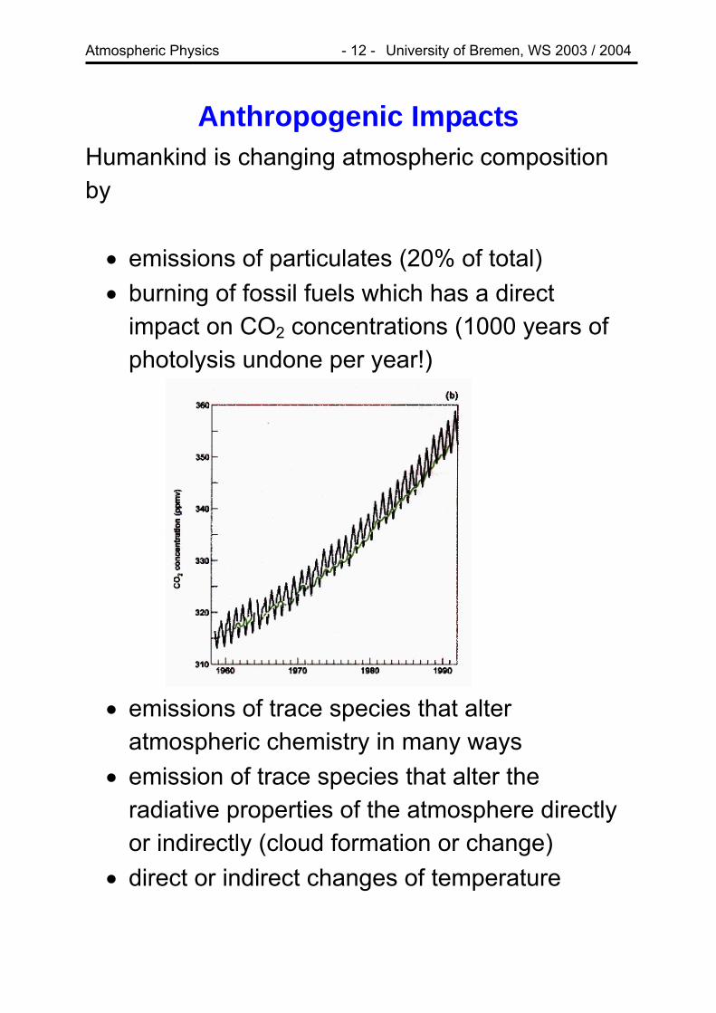
Anthropogenic Impacts Humankind is changing atmospheric composition by • emissions of particulates (20% of total) • burning of fossil fuels which has a direct
impact on CO2 concentrations (1000 years of photolysis undone per year!)
• emissions of trace species that alter
atmospheric chemistry in many ways • emission of trace species that alter the
radiative properties of the atmosphere directly or indirectly (cloud formation or change)
• direct or indirect changes of temperature
Atmospheric Physics - 13 - University of Bremen, WS 2003 / 2004
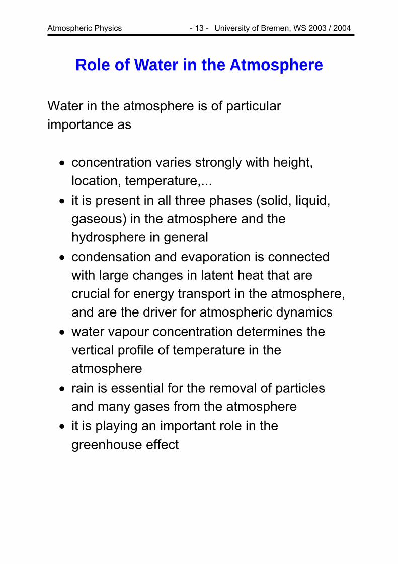
Role of Water in the Atmosphere Water in the atmosphere is of particular importance as • concentration varies strongly with height,
location, temperature,... • it is present in all three phases (solid, liquid,
gaseous) in the atmosphere and the hydrosphere in general
• condensation and evaporation is connected with large changes in latent heat that are crucial for energy transport in the atmosphere, and are the driver for atmospheric dynamics
• water vapour concentration determines the vertical profile of temperature in the atmosphere
• rain is essential for the removal of particles and many gases from the atmosphere
• it is playing an important role in the greenhouse effect

Atmospheric Physics - 14 - University of Bremen, WS 2003 / 2004
Water Vapour in Atmospheres
Water Vapor Pressure [10-1 Nm-1]
Ice
Liquid Water
Vapor
Venus Earth Mars
[K]
T
• Earth is the only planet in the solar system
where water can exist in all three phases. • Most of the water emitted by volcanoes in
Earth’s history is missing (99%) • Only a very small fraction of the water is in the
atmosphere (97% in oceans, 2.4% in ice, 0.6% in underground fresh water, 0.02% in lakes and rivers, and 0.001% the atmosphere)

Atmospheric Physics - 15 - University of Bremen, WS 2003 / 2004
The Atmosphere in Perspective
The atmosphere • is exceedingly thin • contains only a minute fraction of the Earth’s
mass (0.025%), even for its main constituents • Lithosphere (the earth’s crust), Hydrosphere
(water on or above the earth’s surface) and Biosphere (all animal and plant life) act as huge reservoirs for atmospheric constituents

Atmospheric Physics - 16 - University of Bremen, WS 2003 / 2004
Vertical Structure of the Atmosphere
Atmospheric Physics - 17 - University of Bremen, WS 2003 / 2004
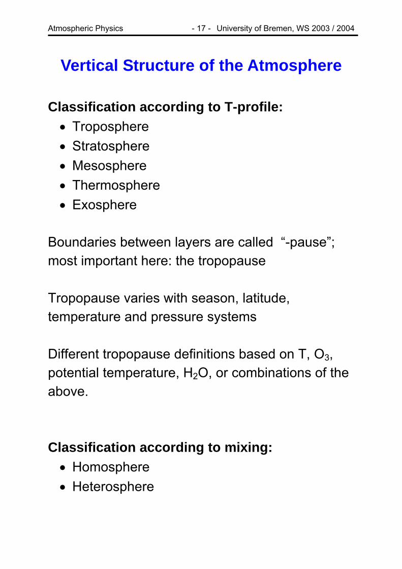
Vertical Structure of the Atmosphere Classification according to T-profile: • Troposphere • Stratosphere • Mesosphere • Thermosphere • Exosphere
Boundaries between layers are called “-pause”; most important here: the tropopause Tropopause varies with season, latitude, temperature and pressure systems Different tropopause definitions based on T, O3, potential temperature, H2O, or combinations of the above. Classification according to mixing: • Homosphere • Heterosphere

Atmospheric Physics - 18 - University of Bremen, WS 2003 / 2004
Vertical Structure of the Atmosphere Reasons for the temperature profile: • adiabatic vertical transport • radiative cooling by water vapour • absorption in the ozone layer • oxygen absorption in the thermosphere
Consequences of the temperature profile: • strong mixing in the troposphere • low vertical mixing in the stratosphere • very low humidity in the stratosphere
(tropopause acts as a cooling trap) • troposphere and stratosphere are largely
separated regions of the atmosphere, and exchange between the two is limited to specific regions:
o through convection in the tropics o in tropopause folds o through subsidence in polar regions

Atmospheric Physics - 19 - University of Bremen, WS 2003 / 2004
Abundance Units in Atmospheric Science
quantity symbol units
number of molecules
N mol = 6.022 x10²³
number density n particles / m3
mass density ρ kg / m3
volume mixing ratio
µ ppmV = 10-6
ppbV = 10-9
pptV = 10-12
mass mixing ratio
µ ppmm =10-6
ppbm =10-9
pptm = 10-12
column abundance
molec/cm2
or DU = 10-3 cm at STP
Atmospheric Physics - 20 - University of Bremen, WS 2003 / 2004
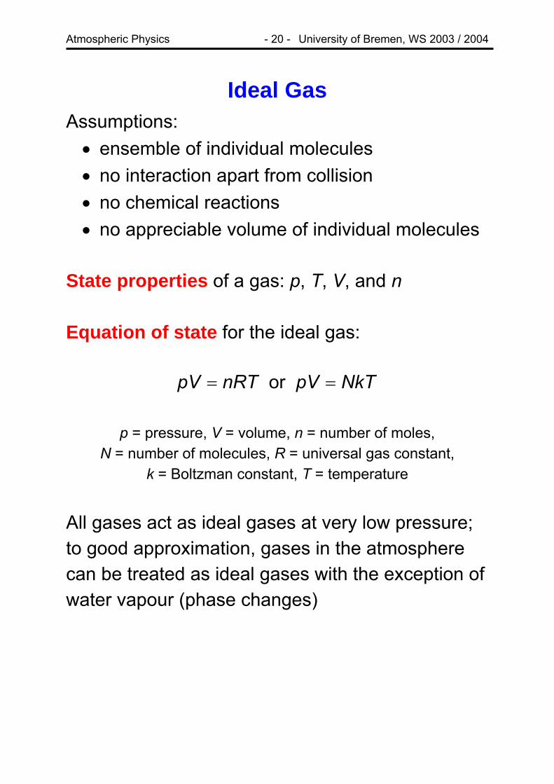
Ideal Gas Assumptions: • ensemble of individual molecules • no interaction apart from collision • no chemical reactions • no appreciable volume of individual molecules
State properties of a gas: p, T, V, and n Equation of state for the ideal gas:
NkTpVnRTpV == or
p = pressure, V = volume, n = number of moles, N = number of molecules, R = universal gas constant,
k = Boltzman constant, T = temperature All gases act as ideal gases at very low pressure; to good approximation, gases in the atmosphere can be treated as ideal gases with the exception of water vapour (phase changes)
Atmospheric Physics - 21 - University of Bremen, WS 2003 / 2004
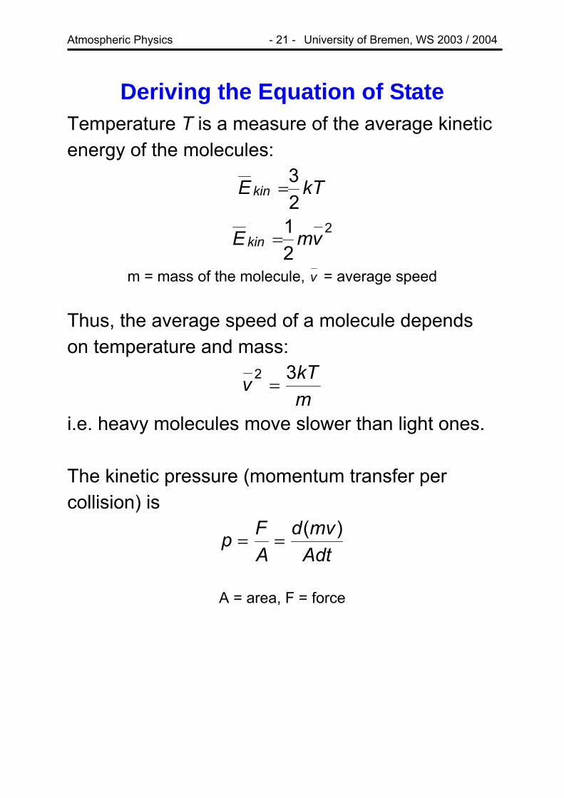
Deriving the Equation of State Temperature T is a measure of the average kinetic energy of the molecules:
kTE kin23=
2
21 vmE kin =
m = mass of the molecule, v = average speed
Thus, the average speed of a molecule depends on temperature and mass:
mkTv 32
=
i.e. heavy molecules move slower than light ones. The kinetic pressure (momentum transfer per collision) is
Adtmvd
AFp )(==
A = area, F = force

Atmospheric Physics - 22 - University of Bremen, WS 2003 / 2004
Change of momentum ∆P for one collision with wall:
xvmP 2=∆
The number of collisions in an interval ∆t is the number of molecules contained in the distance that the molecules travel in ∆t times the area of the wall
tvAVN
x ∆
On average, half of the molecules move to the left, half to the right
tvAVN
x ∆2
The total momentum change then is 22
2 xmvtAVN
∆

Atmospheric Physics - 23 - University of Bremen, WS 2003 / 2004
the rate of change is 2
xAmvVN
and the pressure p=F/A
2xmv
VNp =
Not all particles travel at the same speed, so the average pressure is
2xvm
VNp =
If we consider that no direction is special
22222 3 xzyx vvvvv =++=
we can express the average speed in x-direction
by 2
31v . Combining now the equation for pressure
with the relation between speed and temperature, we get
VNkTv
VNv
VNp x ===
22
3

Atmospheric Physics - 24 - University of Bremen, WS 2003 / 2004
Mixtures of Ideal Gases Dalton’s law: The pressure exerted by a mixture of perfect gases is the sum of the pressures exerted by the individual gases occupying the same volume alone or
BA ppp += Mole fraction: The mole fraction of a gas X in a mixture is the number of moles of X molecules present (nX) as a fraction of the total number of moles of molecules (n) in the sample:
... with +++== CBAX
X nnnnn
nx
Partial pressure: The partial pressure of a gas in a mixture is defined as the product of mole fraction of this gas and total pressure of the gas:
pxp Xx =

Atmospheric Physics - 25 - University of Bremen, WS 2003 / 2004
Excursion: Ideal Gas Law The ideal gas law can be expressed in molecules or moles:
NkTpVnRTpV == or R or R* = Universal gas constant = 8.314 J mol-1 K-1
k = Boltzmann’s constant = 1.381 10-23 J molec-1 K-1
NA = Avogadro’s number = 6.022 1023 mol-1
R = NA k Number density:
kTp
VN
=
Mass density:
RTpM
kTNpM
kTpm
VNm
Vm x
A
xxx =====ρ
mx = Mass of one molecule x, Mx molar mass of x In some books, individual gas constants are defined for each gas:
xx M
RR =

Atmospheric Physics - 26 - University of Bremen, WS 2003 / 2004
Virtual Temperature: Problem: The molecular weight of air is not constant, but changes with water vapour pressure Solution: Define a fictitious virtual temperature, that dry air must have to have the same density that the moist air has at a given pressure. The density of moist air is
''2vd
OHd
Vmm
ρρρ +=+
=
md = mass of dry air, mH2O mass of water vapour where ρd’ is the density dry air would have if it would occupy the volume alone. From the ideal gas equation, the partial pressures of water vapour e and dry air pd can be derived:
OHv MTRe 2/'ρ=
airdd MTRp /'' ρ= and total pressure is epp d += '

Atmospheric Physics - 27 - University of Bremen, WS 2003 / 2004
Inserting into the equation for the density
RTeM
TRepM OHd 2)(
+−
=ρ
⎟⎠
⎞⎜⎝
⎛ −−= )1(1 ερpe
RTpMd with 622.02 ==
d
OH
MM
ε
If we now define a virtual Temperature Tv as
)1)(/(1 ε−−=
peTTv
we can write the equation of state for moist air in the ideal gas form using the molecular weight of dry air:
d
v
MTRp ρ
=
Moist air is less dense than dry air, therefore the virtual temperature is always larger than the real temperature (the difference is usually small). In the future, virtual temperature will be used throughout without special notice.
Atmospheric Physics - 28 - University of Bremen, WS 2003 / 2004
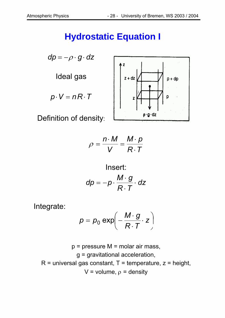
Hydrostatic Equation I
dzgdp ⋅⋅−= ρ
Ideal gas
TRnVp ⋅=⋅
Definition of density:
TRpM
VMn
⋅⋅
=⋅
=ρ
Insert:
dzTRgMpdp ⋅⋅⋅
⋅−=
Integrate:
⎟⎠⎞
⎜⎝⎛ ⋅
⋅⋅
−= zTRgMpp exp0
p = pressure M = molar air mass,
g = gravitational acceleration, R = universal gas constant, T = temperature, z = height,
V = volume, ρ = density

Atmospheric Physics - 29 - University of Bremen, WS 2003 / 2004
In this derivation, the hydrostatic equation follows from an equilibrium between ideal gas pressure and the gravitational force of the total mass of air above. Thus, M is the apparent molar weight of air, and no separation occurs between the constituents. We have also tacitly assumed that • temperature and • gravitational acceleration
do not depend on altitude although that’s clearly not true! Accounting for the temperature profile:
dzzRT
Mgp
dp)(
−=
∫∫ −=zz
zTdz
RMg
pdp
00 )'('
Defining the harmonic mean of T ∫=⎟⎠⎞
⎜⎝⎛ z
zTdz
zT 0 )'('11
⎟⎟⎠
⎞⎜⎜⎝
⎛⎟⎠⎞
⎜⎝⎛−= zTR
Mgpp 1exp0

Atmospheric Physics - 30 - University of Bremen, WS 2003 / 2004
Conclusions for the atmospheric pressure profile: • exponential decay with height • decay is faster at low temperatures
• harmonic mean of T needed instead of arithmetic mean (difference is usually small)
• on larger planets (larger g) pressure decreases faster

Atmospheric Physics - 31 - University of Bremen, WS 2003 / 2004
Hydrostatic Equation II Alternative derivation using Boltzmann statistic: Assume an infinitely high column of air with N0 molecules/area. The potential Energy of one molecule is Epot = mgz The Boltzmann distribution gives the number of molecules in a given energy interval as a function of Temperature:
dEkTECEdN ⎟
⎠⎞
⎜⎝⎛−= exp)(
With we can determine C to ∫ = 0NdnkTNC 0=
Expressing E as function of z
mgzE = and dzmgdE = yields
dzzz
zN
dzzkTmg
kTmgNzdN
⎟⎟⎠
⎞⎜⎜⎝
⎛−=
⎟⎠⎞
⎜⎝⎛−=
00
0
0
exp
exp)(
where z0 is the scale height.
Atmospheric Physics - 32 - University of Bremen, WS 2003 / 2004
Considering that dzzdNzn /)()( = , and setting
000 / zNn = we obtain
⎟⎟⎠
⎞⎜⎜⎝
⎛−=
00 exp)(
zznzn
At constant temperature, 00 /)(/)( pzpnzn = and we obtain the barometric equation. In the real atmosphere, pressure will deviate from this formula depending on the T-profile. This formula, however, is valid for each component of air independently, and heavy gases are closer to the surface than light ones!
Atmospheric Physics - 33 - University of Bremen, WS 2003 / 2004
Geopotential Definition: The Geopotential Φ of any point in the atmosphere is the work that most be done against the earth’s gravitational field in order to raise a mass of 1 kg from sea level to the point.
gdzmgdzd ==Φ and setting Φ(0) = 0
∫=Φz
dzzgz0
)()(
• Φ does not depend on the path used to move
a mass from the sea surface to a point • the differences in geopotential between two
points ΦB - ΦA is the work in the gravitational field needed to move a mass of 1 kg from point A to point B
The geopotential depends on altitude as a result of the distance dependence of the gravitational force.
Atmospheric Physics - 34 - University of Bremen, WS 2003 / 2004
The geopotential also depends on latitude mainly because of the flattening of earth at the poles and the latitudinal dependence of the centrifugal force. From the geopotential, we can also define a Geopotential Height
∫=Φ
=z
dzzggg
zZ000
)(1)(
where g0=9.8 ms-2 is the globally averaged gravitational acceleration at sea surface level. Geopotential height is used as vertical coordinate in most atmospheric applications where energy plays an important role.

Atmospheric Physics - 35 - University of Bremen, WS 2003 / 2004
Measuring the Geoid The 0-point of the geopotential, the geoid also varies with location, mainly as a result of uneven mass distribution in the earth. It can be measured for example from the twin satellites GRACE which monitor their distance (roughly 120 km) with high accuracy. The resulting gravity anomaly (effects of oblateness already subtracted) is important for ocean currents and sea ice mass.

Atmospheric Physics - 36 - University of Bremen, WS 2003 / 2004
Scale Height The factor in the exponent in the hydrostatic equation
⎟⎠⎞
⎜⎝⎛ ⋅
⋅⋅
−= zTRgMpp exp0
has the units of inverse length and is called the Scale Height:
MgRTz =0
Often, the hydrostatic equation is expressed as
( )00 /exp zzpp −= The scale height is the height at which pressure is reduced by a factor of e (2.718); for the atmosphere as a whole it is about 8km which corresponds to a reduction to half the value at 5.5 km. The scale height depends on M and thus is different for different species; also, it depends on T and thereby altitude.

Atmospheric Physics - 37 - University of Bremen, WS 2003 / 2004
Examples for scale heights: Different Planets: Planet name
Major atmospheric constituent
M [g]
g0
[m/s2]Tsurfac
e [K] H [km]
Venus CO2 44 8.9 700 14.9 Earth N2,O2 29 9.8 270 7.9 Mars CO2 44 3.7 210 10.6 Jupiter H2 2 26.2 160 25.3
Different Species
Species Molecular Mass M [g]
Scale height H in [km]
Argon (Ar) 40 21 Nitrogen (N2) 28 30 Atomic Oxygen (O) 16 54 Atomic Hydrogen (H) 1 850

Atmospheric Physics - 38 - University of Bremen, WS 2003 / 2004
Isobaric Atmosphere It is sometimes useful to imagine an atmosphere where everything is brought to surface pressure (and temperature). In such a model atmosphere, the density is constant and equal to the surface density ρ0. The thickness of this atmosphere can be derived from evaluating the total mass
00
000
00 )/exp()(
z
dzzzdzzM
ρ
ρρ
=
−== ∫∫∞∞
and is identical to the scale height z0. This relation is sometimes used to define a scale height for constituents with arbitrary vertical profiles c(z):
∫∞
=00
0 )(1 dzzcc
z
where c0 is the concentration at the surface.

Atmospheric Physics - 39 - University of Bremen, WS 2003 / 2004
Distributions of Speed The Maxwell-Boltzmann distribution of speed is
kTmvx
xekT
mvf 2/2/1
2
2)( −⎟
⎠⎞
⎜⎝⎛=π
The Maxwell distribution of speeds is
kTmvevkT
mvf 2/22/3 2
24)( −
⎟⎠⎞
⎜⎝⎛=π
π
Atmospheric Physics - 40 - University of Bremen, WS 2003 / 2004
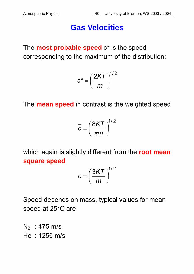
Gas Velocities The most probable speed c* is the speed corresponding to the maximum of the distribution:
2/12* ⎟⎠⎞
⎜⎝⎛=
mKTc
The mean speed in contrast is the weighted speed
2/18⎟⎠⎞
⎜⎝⎛=
mKTcπ
which again is slightly different from the root mean square speed
2/13⎟⎠⎞
⎜⎝⎛=
mKTc
Speed depends on mass, typical values for mean speed at 25°C are N2 : 475 m/s He : 1256 m/s

Atmospheric Physics - 41 - University of Bremen, WS 2003 / 2004
Escape Velocity A moving body (in this case: a molecule) can leave the earth’s gravitational field if its kinetic energy is larger than the potential energy needed to overcome the gravitational field. It depends only on altitude and at 500 km is of the order of 11 km s-1. If the speed of a molecule is high enough, and at the same time the mean free path is long enough, it may leave the atmosphere. The speed depends on temperature and mass, the mean free path on density. Typical values for mean free path are 200 km: 200m 100 km: 15 cm 0 km: 0.06µm Below 100 km (Homosphere), collisions between molecules are so frequent that all constituents are well mixed and no separation is possible. Above that altitude, the different scale heights come into effect (Heterosphere).

Atmospheric Physics - 42 - University of Bremen, WS 2003 / 2004
An example for the un-mixing is given in the figure
At the base of the escape region (Exosphere), temperatures are of the order of 600K. Thus, for atomic hydrogen, the most probable speed is about 3 km s-1. From the Boltzmann distribution, a probability of about 10-6 exists for each collision that an atomic hydrogen is faster than 11 km s-1 an thus can escape the atmosphere. This explains the low atmospheric concentration of hydrogen. For O2, the probability is of the order of 10-84, and thus escape is negligible.
Atmospheric Physics - 43 - University of Bremen, WS 2003 / 2004
Ionosphere At high altitudes (> 60 km), the relative density of ions and electrons increases as a result of ionisation of air molecules by solar X-ray and UV radiation. High energy cosmic rays also contribute to ionisation. This layer is sometimes also called Heaviside Layer. Ionisation increases with altitude as a result of • increased mean free path => increased life
time • increased radiation
The free electrons in the Ionosphere have an impact on radio communication by reflecting or absorbing radio waves and also act a s a Faraday cage against charged particles. Charged particles are also produced in the atmosphere by other processes: • radioactive decay of substances within the
earth’s crust • charge separation within clouds

Atmospheric Physics - 44 - University of Bremen, WS 2003 / 2004
The free electrons make the ionosphere conducting, a so-called plasma. For a given electron density we can calculate the plasma frequency f , this results in the fact that the plasma becomes a reflector for all electromagnetic waves with frequencies pff <
Nconstm
eNfp ==0
12 επ
with the 3109 −⋅≈const , pf in [MHz] and the
electron density N in [cm-3], m the mass of the electron and ε0 the permittivity in vacuum. Therefore for an electron density of
we find a plasma frequency 35103 −⋅= cmNMHzfp 5≈
Region Altitude [km] Electron density [cm3]
(typical, order of magnitude)
D < 90 103-104
E 90 - 140 105
F1
F2
> 140 Maximum of 106 in the region of 250 - 500 km
Atmospheric Physics - 45 - University of Bremen, WS 2003 / 2004
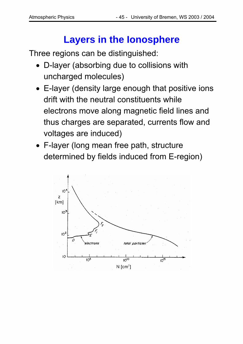
Layers in the Ionosphere Three regions can be distinguished: • D-layer (absorbing due to collisions with
uncharged molecules) • E-layer (density large enough that positive ions
drift with the neutral constituents while electrons move along magnetic field lines and thus charges are separated, currents flow and voltages are induced)
• F-layer (long mean free path, structure determined by fields induced from E-region)
Atmospheric Physics - 46 - University of Bremen, WS 2003 / 2004
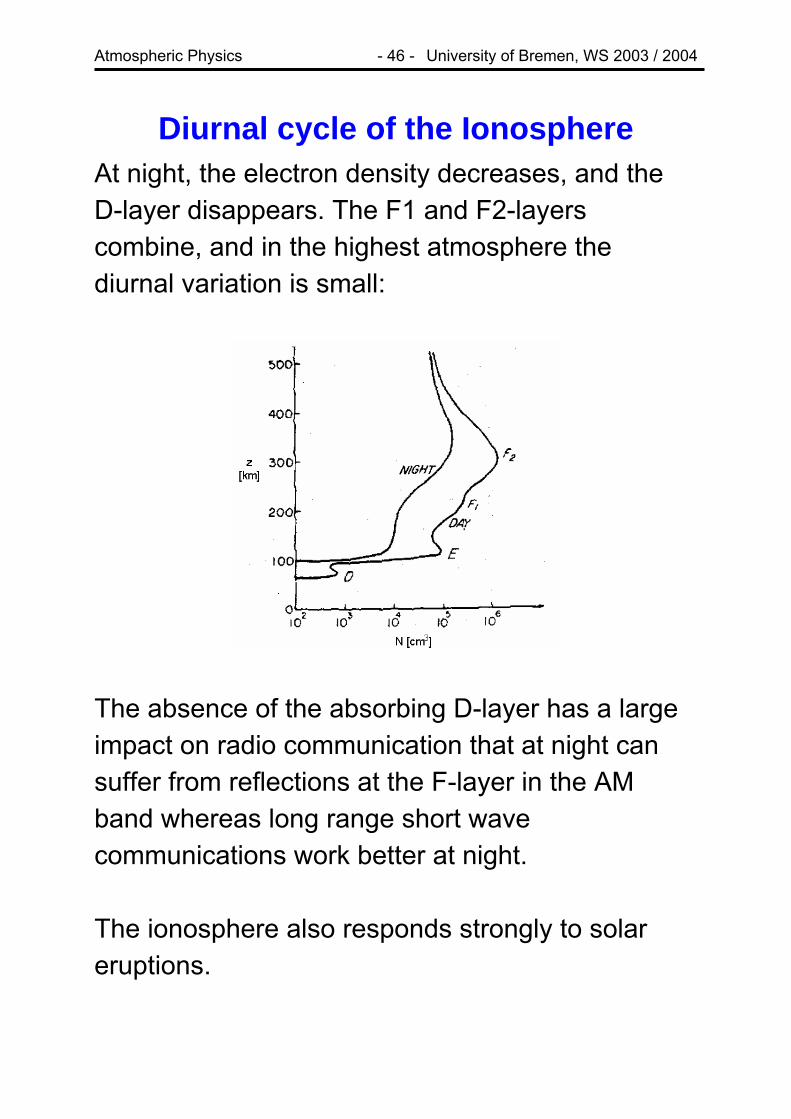
Diurnal cycle of the Ionosphere At night, the electron density decreases, and the D-layer disappears. The F1 and F2-layers combine, and in the highest atmosphere the diurnal variation is small:
The absence of the absorbing D-layer has a large impact on radio communication that at night can suffer from reflections at the F-layer in the AM band whereas long range short wave communications work better at night. The ionosphere also responds strongly to solar eruptions.

Atmospheric Physics - 47 - University of Bremen, WS 2003 / 2004
Extract from http://www.spaceweather.com/ What's Up in Space -- 29 Oct 2003
AURORAS NOW! The coronal mass ejection described below has reached Earth (at approximately 0630 UT on Oct. 29th) and triggered a strong geomagnetic storm. This storm is ongoing! Red and green Northern
Lights have been spotted as far south as Bishop, California. Stay tuned for updates.
EXTREME SOLAR ACTIVITY: One of the most powerful solar flares in years erupted from giant sunspot 486 this morning at approximately 1110 UT. The blast measured X17 on the Richter scale of solar flares. As a result of the explosion, a severe S4-class solar radiation storm is underway. Click here to learn how such storms can affect our planet. The explosion also hurled a coronal mass ejection (CME) toward Earth. When it left the sun, the cloud was traveling 2125 km/s (almost 5 million mph). This CME could trigger bright auroras when it sweeps past our planet perhaps as early as tonight.
Above: This SOHO coronagraph image captured at 12:18 UT shows the coronal mass ejection of Oct. 28th billowing directly toward Earth. Such clouds are called halo CMEs. The many speckles are solar protons striking the coronagraph's CCD camera. See the complete movie.
Where will the auroras appear? High-latitude sites such as New Zealand, Scandinavia, Alaska, Canada and US northern border states from Maine to Washington are favored, as usual, but auroras could descend to lower latitudes when the CME pictured above sweeps past Earth.
Right: Photographer Lance Taylor of Alberta, Canada, spotted these vivid Northern Lights on Oct. 21st. [gallery]
Not all CMEs trigger auroras. Several, for instance, have swept past Earth in recent days without causing widespread displays. It all depends on the orientation of tangled magnetic fields within the electrified cloud of gas. The incoming CME is no exception. It might cause auroras, or it might not. We will find out when it arrives.

Atmospheric Physics - 48 - University of Bremen, WS 2003 / 2004
Probing the Ionosphere The electron density in the Ionosphere can be studied from the ground (and from space) by emitting radio signals at different frequencies and measuring the time lag of the reflected signal (Ionosonde):
To reach higher altitudes, the frequency is increased. Absorption in the D-layer can not be studied in this way.

Atmospheric Physics - 49 - University of Bremen, WS 2003 / 2004
Magnetosphere Above 500 km, collisions are infrequent and the magnetic field determines the motion of charged particles. Earth’s magnetic field is approximately a dipole with 11° inclination to the rotation axis. Solar wind distorts the magnetic field:
Solar outbursts impact the magnetic field and inject high energy particles into the lower ionosphere, which gives rise to brilliant auroral displays. The magnetic field provides an important shield from solar wind.
Atmospheric Physics - 50 - University of Bremen, WS 2003 / 2004
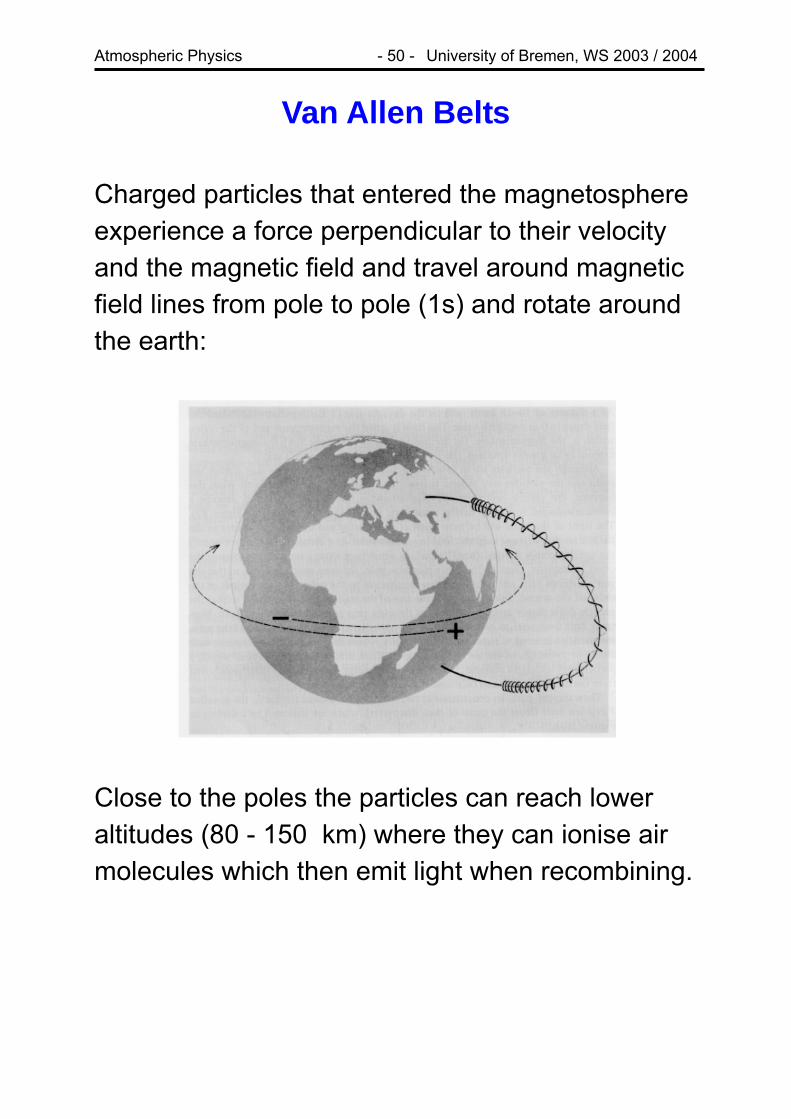
Van Allen Belts Charged particles that entered the magnetosphere experience a force perpendicular to their velocity and the magnetic field and travel around magnetic field lines from pole to pole (1s) and rotate around the earth:
Close to the poles the particles can reach lower altitudes (80 - 150 km) where they can ionise air molecules which then emit light when recombining.
Atmospheric Physics - 51 - University of Bremen, WS 2003 / 2004
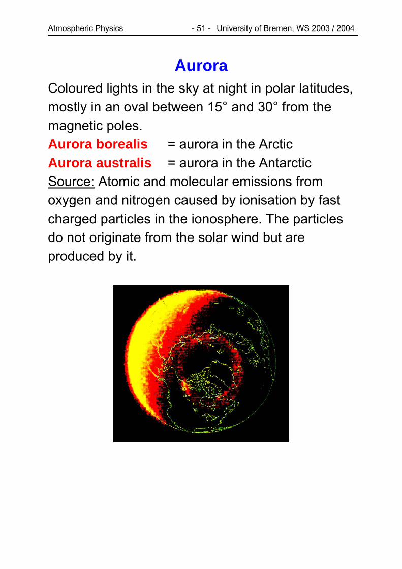
Aurora Coloured lights in the sky at night in polar latitudes, mostly in an oval between 15° and 30° from the magnetic poles. Aurora borealis = aurora in the Arctic Aurora australis = aurora in the Antarctic Source: Atomic and molecular emissions from oxygen and nitrogen caused by ionisation by fast charged particles in the ionosphere. The particles do not originate from the solar wind but are produced by it.

Atmospheric Physics - 52 - University of Bremen, WS 2003 / 2004
Earth in Space
• Earth’s orbit around the sun is slightly elliptic
(149.6x10⁶ km - 152x106 km) • Earth’s ecliptic is 23.5° • seasons are result of ecliptic, not elliptic orbit • during summer, there is polar day polewards of
the arctic cycle, depending on date • during winter, the pole is without solar
illumination (polar night • twice per year, there is equinox (21.3. and
23.9.)
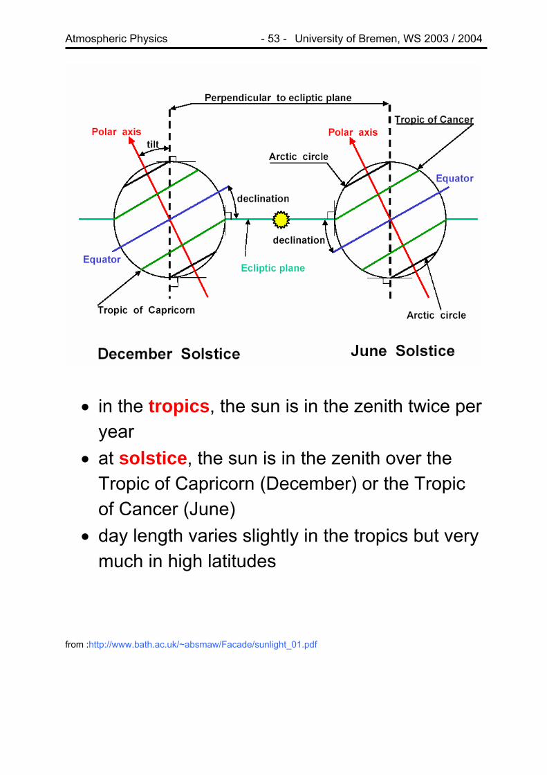
Atmospheric Physics - 53 - University of Bremen, WS 2003 / 2004
• in the tropics, the sun is in the zenith twice per
year • at solstice, the sun is in the zenith over the
Tropic of Capricorn (December) or the Tropic of Cancer (June)
• day length varies slightly in the tropics but very much in high latitudes
from :http://www.bath.ac.uk/~absmaw/Facade/sunlight_01.pdf

Atmospheric Physics - 54 - University of Bremen, WS 2003 / 2004
The Electromagnetic Spectrum
Wavelength λ I I i I I I I I I I I I I I 1km 100m 10m 1m 0.1m 10cm 1cm 1mm 0.1mm 10µm 1µm 0.1µm 10nm 1nm Radiowaves Microwaves thermal X-ray Infrared Visible Ultraviolet Interaction of electromagnetic Rotation Vibration Electron radiation with matter Transition
• nearly all energy on Earth is supplied by the
sun through radiation • wavelengths from many meters (radio waves)
to nm (X-ray) • small wavelength = high energy • radiation interacts with atmosphere
o absorption (heating, shielding) o excitation (energy input, chemical
reactions) o re-emission (energy balance o remote sensing applications

Atmospheric Physics - 55 - University of Bremen, WS 2003 / 2004
Radiation can be characterized by its wavelength, λ [m] and the frequency ν [Hz]. The two quantities are related by
λ
ν c=
with c = 2.9979250x10⁸ m/s the speed of light Sometimes (in particular in the IR), wavenumber k is used instead of frequency:
λπ2
=k
The energy of a photon is determined by the frequency:
E = hν
Name Other commonly used names
Unit Symbol
Radiant flux W P Irradiance Total Flux Wm-2 E Radiance Wm-2sr-1 I Monochromatic Irradiance
Monochromatic Flux
Wm-2 m-1 Eλ
Monochromatic Radiance
Monochromatic Intensity
Wm-2 m-1 sr-1 Iλ

Atmospheric Physics - 56 - University of Bremen, WS 2003 / 2004
Radiometric Definitions:
from http://www.profc.udec.cl/~gabriel/tutoriales/rsnote/cp1/1-6-1.gif

Atmospheric Physics - 57 - University of Bremen, WS 2003 / 2004
Black Body Radiation A black body is a body or gas volume that • has constant temperature • absorbs all incoming radiation completely • has the maximum possible emission in all
directions and at all wavelengths Planck’s law:
⎟⎠⎞
⎜⎝⎛ −⎟
⎠⎞
⎜⎝⎛
=1exp
2)(5
2
λλ
πλ
kThc
hcTE [Wm-2 m-1]
Eλ irradiance h Planck’s constant c speed of light λ wavelength k Boltzmann’s constant T temperature Approximations: Rayleigh-Jeans law (at long wavelengths) Wien’s law (short wavelengths)
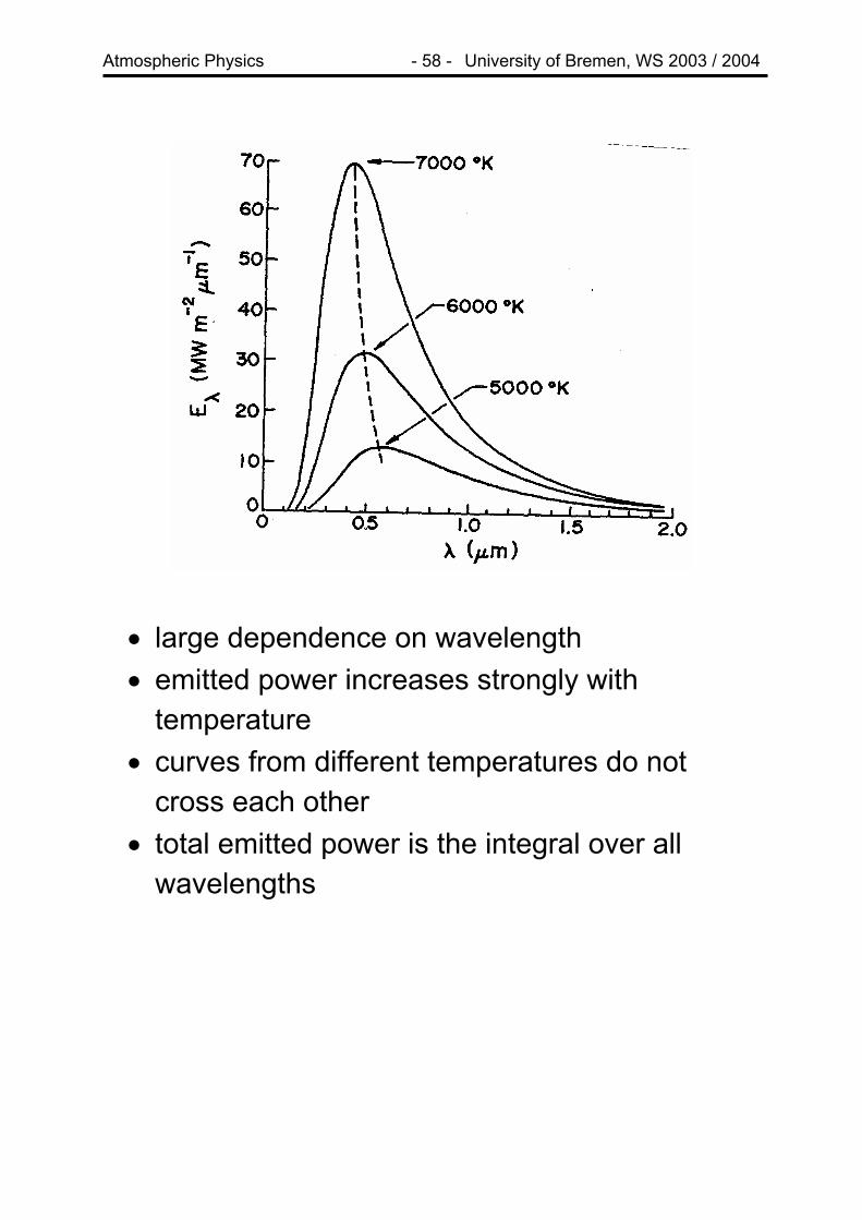
Atmospheric Physics - 58 - University of Bremen, WS 2003 / 2004
• large dependence on wavelength • emitted power increases strongly with
temperature • curves from different temperatures do not
cross each other • total emitted power is the integral over all
wavelengths
Atmospheric Physics - 59 - University of Bremen, WS 2003 / 2004
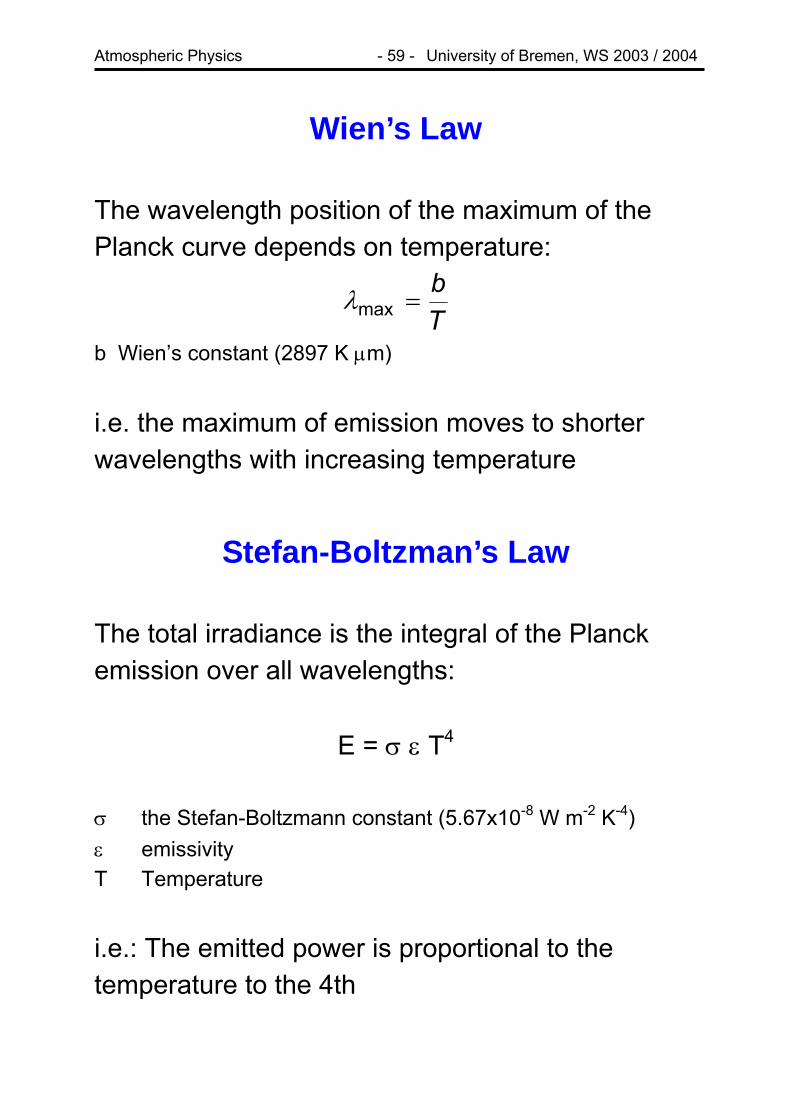
Wien’s Law The wavelength position of the maximum of the Planck curve depends on temperature:
Tb
=maxλ
b Wien’s constant (2897 K µm) i.e. the maximum of emission moves to shorter wavelengths with increasing temperature
Stefan-Boltzman’s Law The total irradiance is the integral of the Planck emission over all wavelengths:
E = σ ε T4
σ the Stefan-Boltzmann constant (5.67x10⁻⁸ W m-2 K-4) ε emissivity T Temperature i.e.: The emitted power is proportional to the temperature to the 4th

Atmospheric Physics - 60 - University of Bremen, WS 2003 / 2004
Kirchhoff’s Law A body with wavelength independent emissivity < 1 is called grey. absorptivity α(λ) emissivity ε(λ) reflectivity ρ(λ) transmissivity τ(λ)
α (λ) + ρ(λ) + τ(λ) = 1 At the same wavelength, absorptivity and emissivity are identical:
α(λ) = ε(λ)
The emission of a body is proportional to its emissivity:
E(λ) = ε(λ) Eblack(λ) If a body is black or white depends on wavelength - snow e.g. is black in the IR! The best approximation for a black body is a cavity.
Atmospheric Physics - 61 - University of Bremen, WS 2003 / 2004
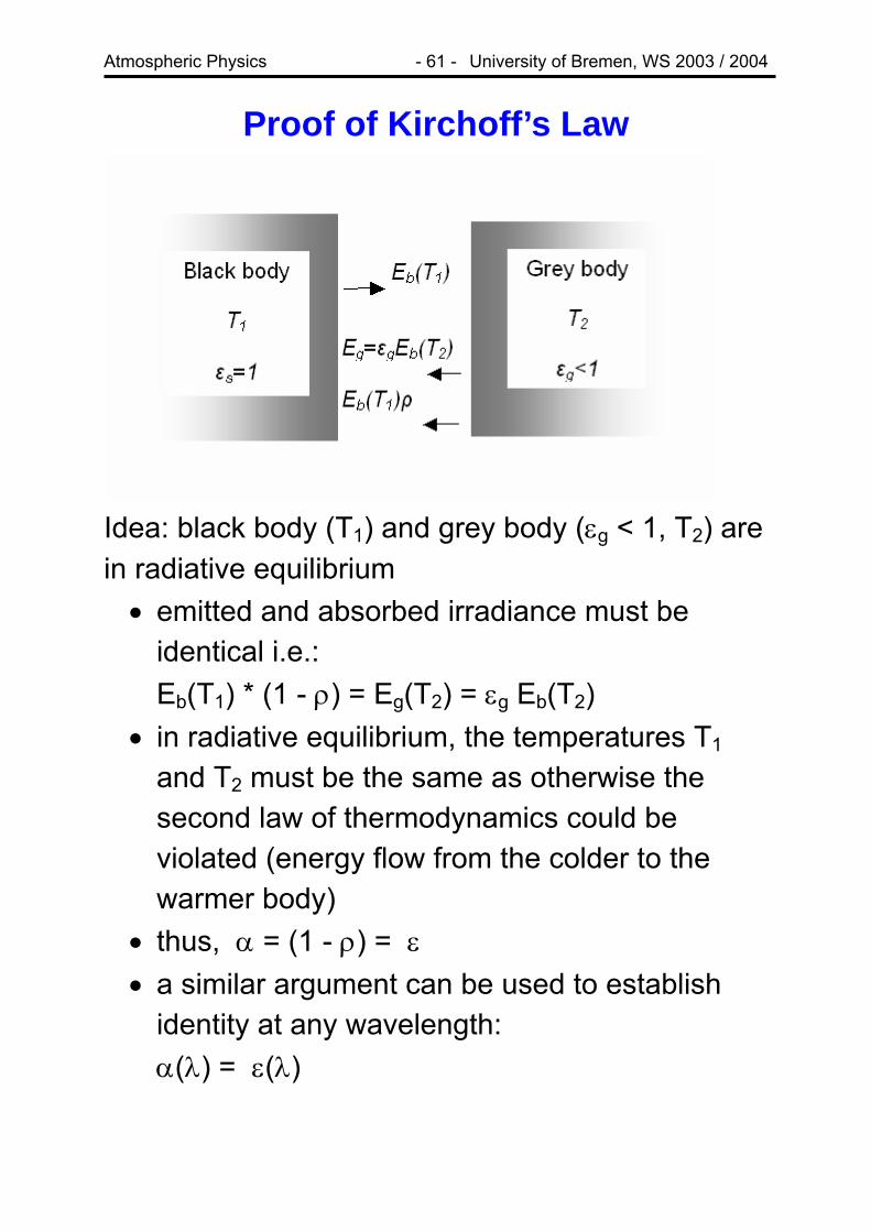
Proof of Kirchoff’s Law
Idea: black body (T1) and grey body (εg < 1, T2) are in radiative equilibrium • emitted and absorbed irradiance must be
identical i.e.: Eb(T1) * (1 - ρ) = Eg(T2) = εg Eb(T2)
• in radiative equilibrium, the temperatures T1 and T2 must be the same as otherwise the second law of thermodynamics could be violated (energy flow from the colder to the warmer body)
• thus, α = (1 - ρ) = ε • a similar argument can be used to establish
identity at any wavelength: α(λ) = ε(λ)
Atmospheric Physics - 62 - University of Bremen, WS 2003 / 2004
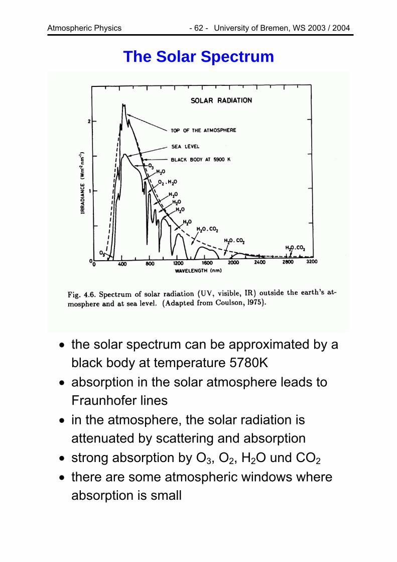
The Solar Spectrum
• the solar spectrum can be approximated by a
black body at temperature 5780K • absorption in the solar atmosphere leads to
Fraunhofer lines • in the atmosphere, the solar radiation is
attenuated by scattering and absorption • strong absorption by O3, O2, H2O und CO2 • there are some atmospheric windows where
absorption is small

Atmospheric Physics - 63 - University of Bremen, WS 2003 / 2004
Solar Spectrum and Earth Spectrum
Sun Earth Short Wave Long Wave
• solar spectrum and earth spectrum have
nearly no overlap • earth spectrum is not to scale, it is below
the solar spectrum at all wavelengths!

Atmospheric Physics - 64 - University of Bremen, WS 2003 / 2004
Planetary Equilibrium Temperatures The radiant flux from the sun P can be computed from the irradiance:
P = A E = 4 π Rsun2σT4
= 3.84x1026 W Rsun = 6.95x10⁸ m Tsun = 5780K
In the distance earth has from the sun, the solar irradiance is called the solar constant Fearth
Fearth = Psun / Asphere = Psun /4π R2earth-sun=1376 W m-2
Rearth-sun = 1.49x10¹¹ m
For a planet in arbitrary distance, the radiant flux P received is
22 )1(
RFrP ρπ −=
P : solar radiant flux absorbed by the planet r : radius of planet ρ : reflectivity or albedo of the planet
R :distance of the planet from the sun, normalized to the sun-earth distance = 1 FEarth : solar constant

Atmospheric Physics - 65 - University of Bremen, WS 2003 / 2004
Assuming radiative equilibrium, the energy received by the sun must be balanced by the thermal emission I of the planet:
424 TrI σπ=
(Note that radiation is emitted in all directions but received only by the area illuminated by the sun). Solving for the equilibrium temperature yields the following values:
Planet Calculated Temperature [K]
Measured Temperature [K]
Venus 227 230 Earth 255 250 Mars 216 220 Jupiter 98 130
Here, the measured temperature is the apparent temperature as seen from space, not the surface temperature.
Atmospheric Physics - 66 - University of Bremen, WS 2003 / 2004
Radiative Transfer in the Atmosphere Contributions: • Direct Solar Ray • Reflection on the Surface • Reflection from Clouds • Scattering in the Atmosphere
o Rayleigh Scattering o Mie Scattering o Raman Scattering
• Absorption in the Atmosphere • Emission in the Atmosphere • Emission from the Surface • Emission from Clouds

Atmospheric Physics - 67 - University of Bremen, WS 2003 / 2004
Absorption in the Atmosphere Absorption in a volume is proportional to • I0 initial radiance • ds light path • n number density of absorbers [m-3] • σa(λ) absorption cross-section [m2]
dI = - I0 σa(λ) n ds ka = n σa is the absorption coefficient [m-1] Integration along the light path leads to Lambert Beer’s law:
⎟⎟⎠
⎞⎜⎜⎝
⎛−= ∫
s
a dsskIsI0
')'(exp)0()(
and for a homogeneous atmosphere
I(s) = I0 exp(-ka s)

Atmospheric Physics - 68 - University of Bremen, WS 2003 / 2004
The integrated absorption is called Opacity or Optical Depth τ:
∫=S
a dssks0
)()(τ
The transmissivity t(s) is
))(exp()0()()( s
IsIst τ−==
and the absorptivity a(s)
)(1)(1
stsaat
−==+
for an opacity τ → ∞ the absorptivity a → 1, this is called the optically “thick” case. Note: σa, τ, t and a can be functions of the wavelength λ.

Atmospheric Physics - 69 - University of Bremen, WS 2003 / 2004
Scattering in the Atmosphere If a photon is absorbed and then immediately re-emitted we have scattering. Mechanisms of Scattering are: • Rayleigh-Scattering • Mie-Scattering • Geometric Optics • (Inelastic Raman-Scattering)
Usually, scattered photons have the same wavelength (elastic scattering) but not the same direction as the original photon.
The phase function P(ϕ) gives the distribution of scattered intensity as a function of scattering angle; the integral over all wavelengths is 1.
Atmospheric Physics - 70 - University of Bremen, WS 2003 / 2004
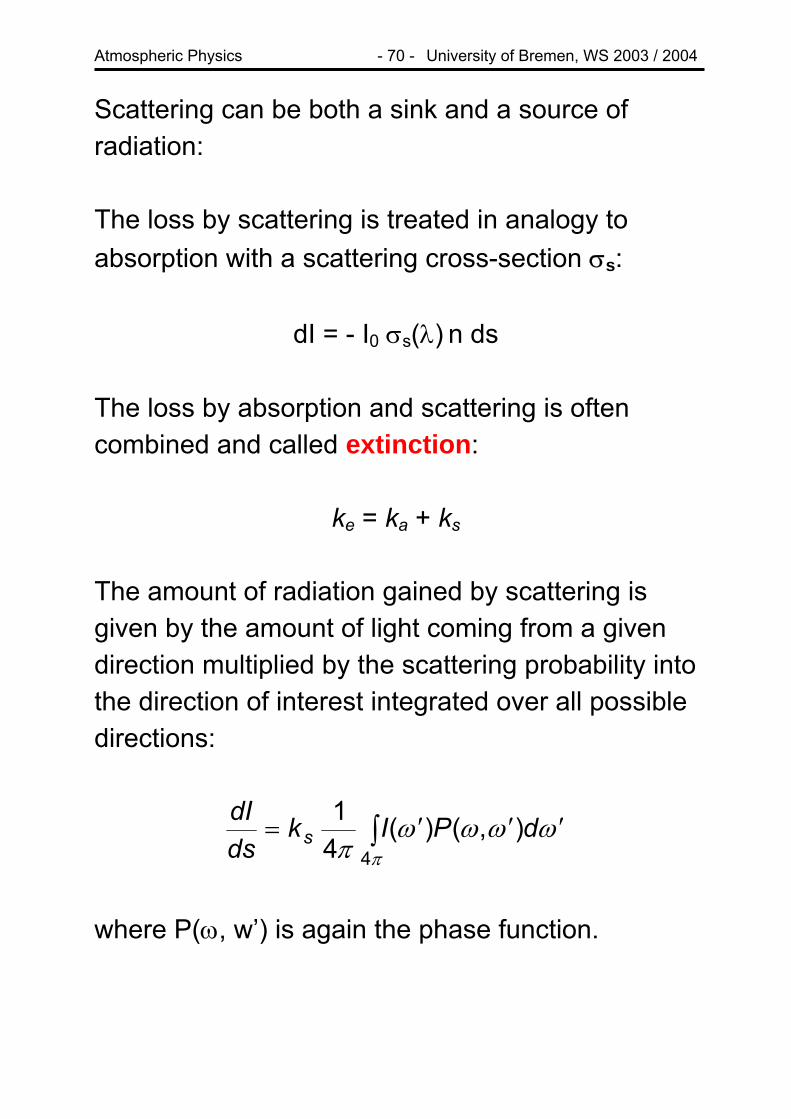
Scattering can be both a sink and a source of radiation: The loss by scattering is treated in analogy to absorption with a scattering cross-section σs:
dI = - I0 σs(λ) n ds The loss by absorption and scattering is often combined and called extinction:
ke = ka + ks
The amount of radiation gained by scattering is given by the amount of light coming from a given direction multiplied by the scattering probability into the direction of interest integrated over all possible directions:
∫ ′′′=π
ωωωωπ 4
),()(41 dPIk
dsdI
s
where P(ω, w’) is again the phase function.
Atmospheric Physics - 71 - University of Bremen, WS 2003 / 2004
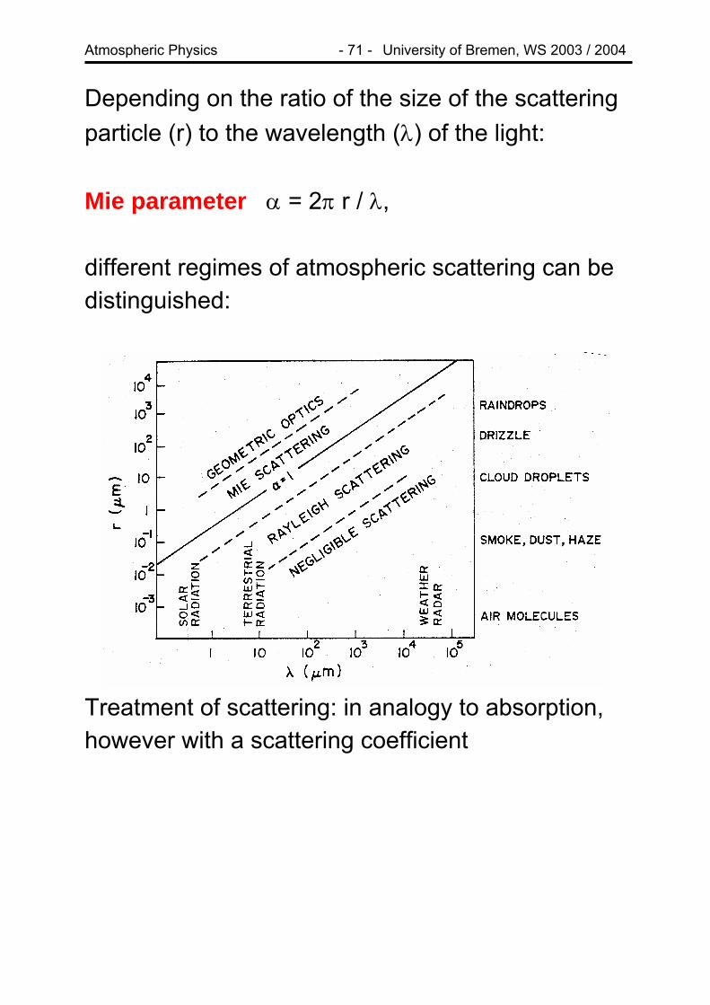
Depending on the ratio of the size of the scattering particle (r) to the wavelength (λ) of the light: Mie parameter α = 2π r / λ, different regimes of atmospheric scattering can be distinguished:
Treatment of scattering: in analogy to absorption, however with a scattering coefficient
Atmospheric Physics - 72 - University of Bremen, WS 2003 / 2004
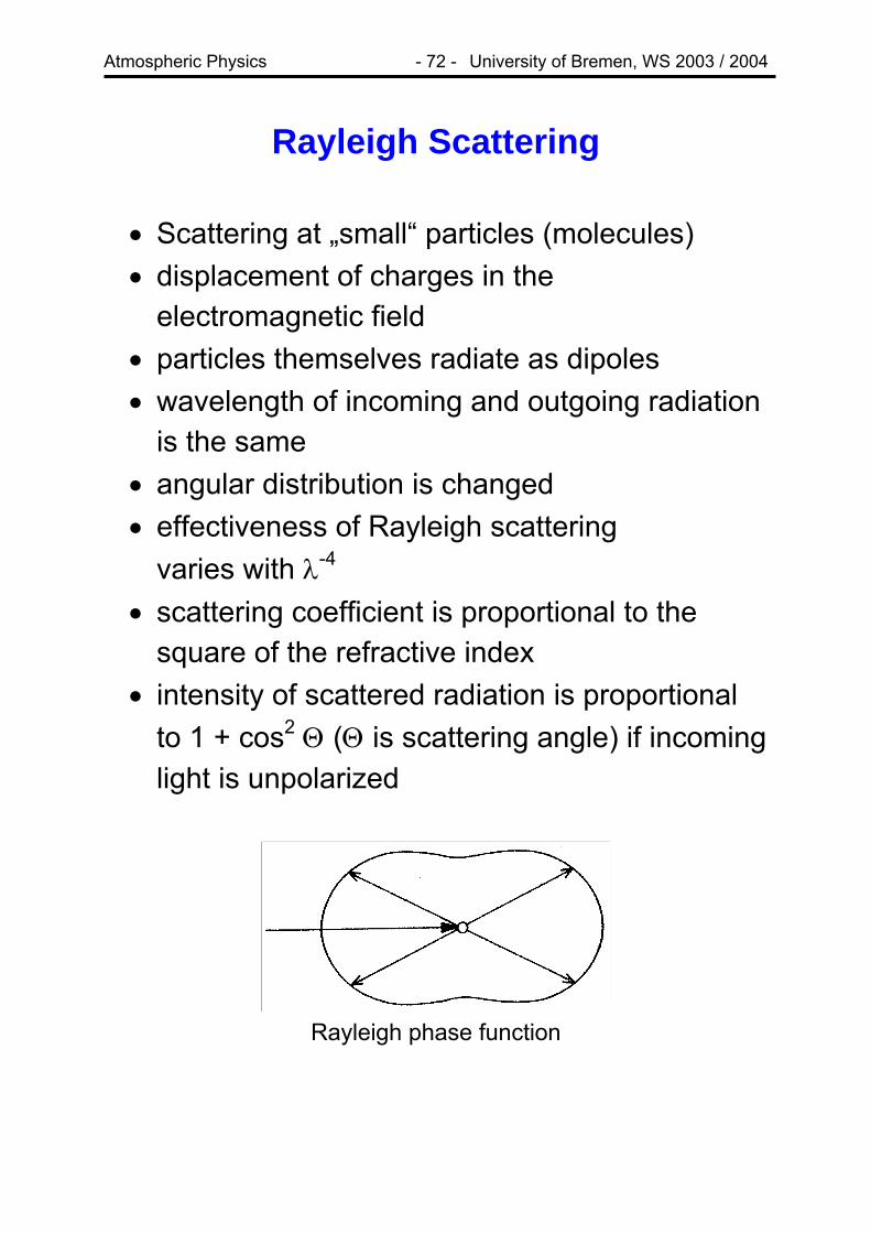
Rayleigh Scattering • Scattering at „small“ particles (molecules) • displacement of charges in the
electromagnetic field • particles themselves radiate as dipoles • wavelength of incoming and outgoing radiation
is the same • angular distribution is changed • effectiveness of Rayleigh scattering
varies with λ-4 • scattering coefficient is proportional to the
square of the refractive index • intensity of scattered radiation is proportional
to 1 + cos2 Θ (Θ is scattering angle) if incoming light is unpolarized
Rayleigh phase function

Atmospheric Physics - 73 - University of Bremen, WS 2003 / 2004
• light is mainly scattered in the forward or backward direction
• Rayleigh scattered light is strongly polarised for 90° scattering angle
Rayleigh scattering can be explained in terms of an ensemble of dipole emitters. A more accurate treatment has to be based on density fluctuations in the scattering medium.

Atmospheric Physics - 74 - University of Bremen, WS 2003 / 2004
Geometry for Rayleigh Scattering
• the atmosphere appears blue as short
wavelengths are scattered more efficiently • UV radiation usually is scattered before
reaching the surface • skylight is polarised perpendicular to the plane
formed by the sun, the observer and the scattering molecule
• the maximum of polarisation is reached at 90° scattering angle

Atmospheric Physics - 75 - University of Bremen, WS 2003 / 2004
Mie Scattering • scattering on „large“ particles (aerosols,
droplets, suspended matter in liquids) • explained by coherent scattering from many
individual particles • for spherical particles, Mie scattering can be
computed from the refractive index using the Maxwell equations
• wavelength of incoming radiation is not changed
• angular distribution is changed
• depending on α, forward scatterfavoured
• effectiveness of Mie scattering isto λ-1 to λ-1.5
• in general. Mie scattering is not
Mie phase function for typical clouddroplet size distribution
ing is strongly
proportional
polarising

Atmospheric Physics - 76 - University of Bremen, WS 2003 / 2004
Phase function for Mie Scattering
• angular distribution is a complex function of
particle size even for spherical particles • the larger the particles, the stronger the
forward scattering peak • Mie scattering leads to „whitening“

Atmospheric Physics - 77 - University of Bremen, WS 2003 / 2004
Extinction by Mie Scattering
In general, Mie scattering can not be treated quantitatively as • most particles are not spherical • the composition of particles is in general not
known • the size distribution of particles is in general
not known • changes in humidity can have a strong impact
on the optical properties • absorption in aerosols can in general not be
neglected

Atmospheric Physics - 78 - University of Bremen, WS 2003 / 2004
Geometric Optics When the wavelength is much smaller than the particle dimension (α >> 1) geometric optics apply. This situation is not very important in the atmosphere, but can lead to nice visual effects such as the rainbow. Rainbows are created by the refraction of light in water droplets. Three rainbows exist: One at 41° around the point opposite of the sun, a second, inverted one with 51° and a third one with a radius of 140° in the direction of the sun.
Geometrical considerations lead to the critical angles, at which light is concentrated and thus a bright rainbow is visible.

Atmospheric Physics - 79 - University of Bremen, WS 2003 / 2004
A similar effect is created by ice crystals and called Halo:
Atmospheric Physics - 80 - University of Bremen, WS 2003 / 2004
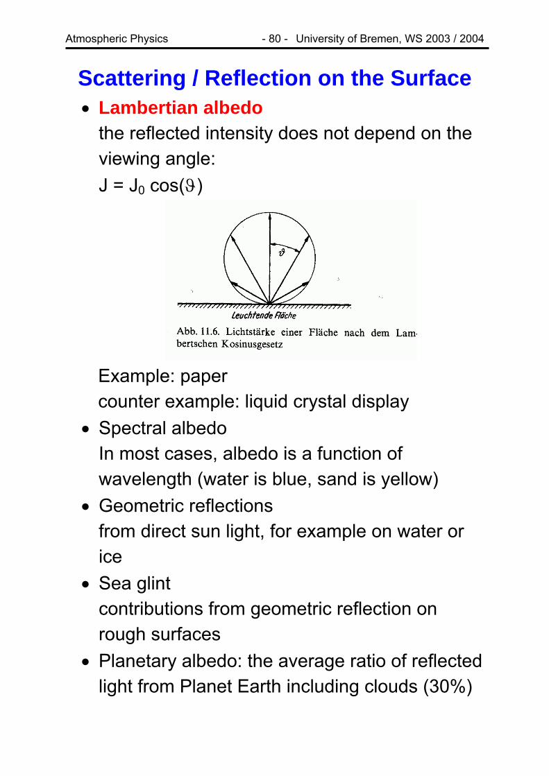
Scattering / Reflection on the Surface • Lambertian albedo
the reflected intensity does not depend on the viewing angle: J = J0 cos(ϑ)
Example: paper counter example: liquid crystal display
• Spectral albedo In most cases, albedo is a function of wavelength (water is blue, sand is yellow)
• Geometric reflections from direct sun light, for example on water or ice
• Sea glint contributions from geometric reflection on rough surfaces
• Planetary albedo: the average ratio of reflected light from Planet Earth including clouds (30%)
Atmospheric Physics - 81 - University of Bremen, WS 2003 / 2004
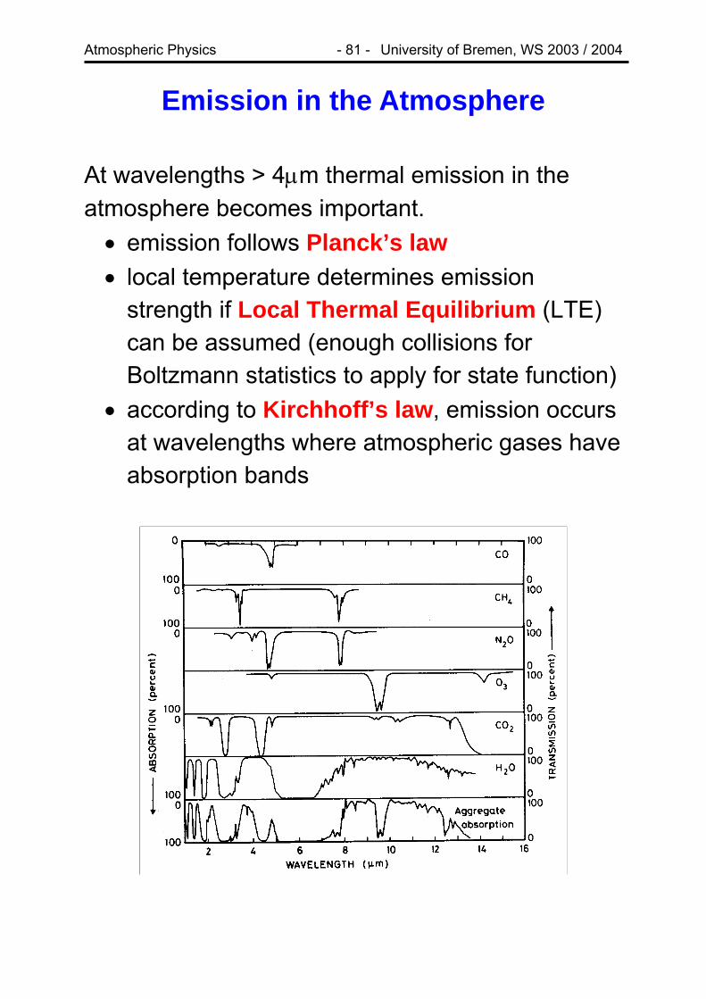
Emission in the Atmosphere At wavelengths > 4µm thermal emission in the atmosphere becomes important. • emission follows Planck’s law • local temperature determines emission
strength if Local Thermal Equilibrium (LTE) can be assumed (enough collisions for Boltzmann statistics to apply for state function)
• according to Kirchhoff’s law, emission occurs at wavelengths where atmospheric gases have absorption bands

Atmospheric Physics - 82 - University of Bremen, WS 2003 / 2004
Radiative Transfer Equation The change in intensity for radiation propagating through a medium is given by
4444 34444 2132143421
sourcescatteringsourcethermalextinction
sa dPITBIkkdsdI
∫ ′′′+++−=π
ωωωωπ
α4
),()(21)()(
where • all quantities depend on wavelength • ka, ks, α and P depend on the composition of
the medium • B(T) and also ka depend on temperature
Atmospheric Physics - 83 - University of Bremen, WS 2003 / 2004
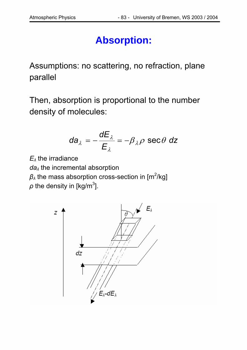
Absorption:
Assumptions: no scattering, no refraction, plane parallel Then, absorption is proportional to the number density of molecules:
dzE
dEda θρβλ
λ
λλ sec−=−=
Eλ the irradiance daλ the incremental absorption βλ the mass absorption cross-section in [m2/kg] ρ the density in [kg/m3].

Atmospheric Physics - 84 - University of Bremen, WS 2003 / 2004
Integrating from altitude z to infinity
∫∞
∞ =−z
dzEE ρβθ λλλ seclnln ,
θρβττ λλλλλ sec)exp(, ⎟⎟⎠
⎞⎜⎜⎝
⎛=−= ∫
∞
∞z
dzwithEE
The transmissivity and absorptivity of a gas layer are given by
( ) λλλλ
λλ τ ta
EE
t −=−==∞
1;exp,
The relation between absorption and optical depth can be linearized for small absorptions ( λλ τ≈a ) but becomes highly nonlinear at large absorptions:

Atmospheric Physics - 85 - University of Bremen, WS 2003 / 2004
Where is most radiation absorbed? At high altitudes, the intensity is large, but the number of absorbers / scatterers small. At low altitudes, the opposite is true. In between the change in radiation has a maximum, roughly at an opacity of 1.
This can also be shown quantitatively (see Wallace and Hobbs or the Script by Künzi and Buehler).
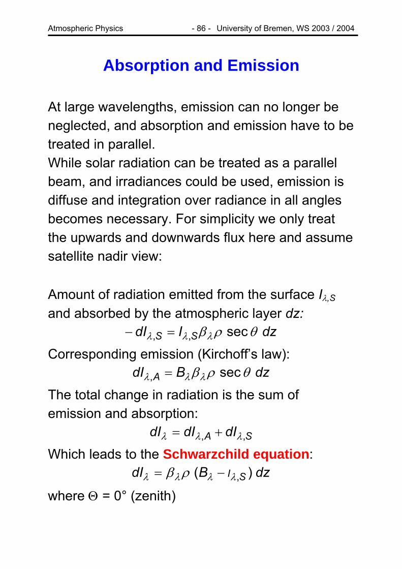
Atmospheric Physics - 86 - University of Bremen, WS 2003 / 2004
Absorption and Emission At large wavelengths, emission can no longer be neglected, and absorption and emission have to be treated in parallel. While solar radiation can be treated as a parallel beam, and irradiances could be used, emission is diffuse and integration over radiance in all angles becomes necessary. For simplicity we only treat the upwards and downwards flux here and assume satellite nadir view: Amount of radiation emitted from the surface Iλ,S and absorbed by the atmospheric layer dz:
dzIdI SS θρβλλλ sec,, =−
Corresponding emission (Kirchoff’s law): dzBdI A θρβλλλ sec, =
The total change in radiation is the sum of emission and absorption:
SA dIdIdI ,, λλλ +=
Which leads to the Schwarzchild equation: dzBdI SI )( ,λλλλ ρβ −=
where Θ = 0° (zenith)

Atmospheric Physics - 87 - University of Bremen, WS 2003 / 2004
When looking at the atmosphere from space, the total radiance from surface and atmosphere is (neglecting scattering):
One layer in the atmosphere: Surface:
)exp(exp' 0,0
,, τρβ λλλλ −=⎟⎟⎠
⎞⎜⎜⎝
⎛−= ∫
∞
SSS IdzII
Total Radiance at top of atmosphere:
∫∞
−+−=0
0, )exp()exp( dzBII STotal τρβτ λλλ

Atmospheric Physics - 88 - University of Bremen, WS 2003 / 2004
Satellite measurements of temperature Idea: For a well mixed absorber (O2, CO2) the βλ is independent of altitude, and the only height dependency is from the known vertical density profile and the Planck emission, which depends on temperature.
Density: ⎟⎠⎞
⎜⎝⎛−=
Hzz exp)( 0ρρ
If the surface term can be neglected (optically thick atmosphere), the radiance at top of atmosphere is
∫ ∫∞ ∞
⎟⎟⎠
⎞⎜⎜⎝
⎛⎟⎠⎞
⎜⎝⎛−−⎟
⎠⎞
⎜⎝⎛−=
000,, ''expexp)( dzdz
Hz
HzzBI
ztotalA λλλλ βρβρ
It is convenient to combine all terms with the exception of Bλ in the Weighting Function W(λ, z), leading to
∫∞
=0
,, )(),( dzzBzWI totalA λλ λ

Atmospheric Physics - 89 - University of Bremen, WS 2003 / 2004
Weighting functions for a nadir looking space borne sensor observing thermal radiation emitted by CO2 near the strong 15 µm band. • different wavelengths have peak contributions
from different altitudes • the latitude depends on the absorption - larger
absorption leads to higher peak • deduction of temperature profile necessitates
“inversion” If the temperature distribution is known, a vertical absorber profile can be retrieved!

Atmospheric Physics - 90 - University of Bremen, WS 2003 / 2004
Selective Absorbers / Emitters • A black body absorbs at all wavelengths with
maximum efficiency (α = 1) • A grey body has a wavelength independent
absorptivity of α < 1 • A selective absorber has a wavelength
dependent absorptivity α(λ) All relevant absorbers in the atmosphere on the surface are selective (coloured). Most important for the atmospheric radiation budget: absorbers that have different absorptivity in the short wave and long wave region. If a surface has large absorptivity at short wavelengths (where energy from the sun is abundant) and a small absorptivity at long wavelengths (where energy is lost through radiation), it will become warmer than a black body. If the opposite is true (e.g. snow), it will become colder than a black body.

Atmospheric Physics - 91 - University of Bremen, WS 2003 / 2004
The atmosphere acts as an selective absorber, as absorption by trace species is large in the IR but small in the visible:
In the IR, the atmosphere is opaque with the exception of two small atmospheric windows at 8µm and 12µm.

Atmospheric Physics - 92 - University of Bremen, WS 2003 / 2004
Greenhouse Effect
With an atmosphere with large IR absorption, the surface receives the solar short wave radiation plus the IR counterradiation, and thus in radiative equilibrium is at higher temperature than without atmosphere. A rough estimate yields:
( )00
40
40
40
40
2.12
2
TTTTT
TE
≈=′
′=
=
σσ
σ
or an increase from 285K => 300 K. Note that agricultural greenhouse mainly works by reducing heat loss through convection and advection.

Atmospheric Physics - 93 - University of Bremen, WS 2003 / 2004
Example: Atmospheric emission spectra from Mars and Earth:
• in the cold polar regions, the atmosphere on
Mars appears warmer than the cold surface • in mid-latitudes, the opposite is true • in Earth’s atmosphere, emissions from O3 and
H2O are also evident
Atmospheric Physics - 94 - University of Bremen, WS 2003 / 2004
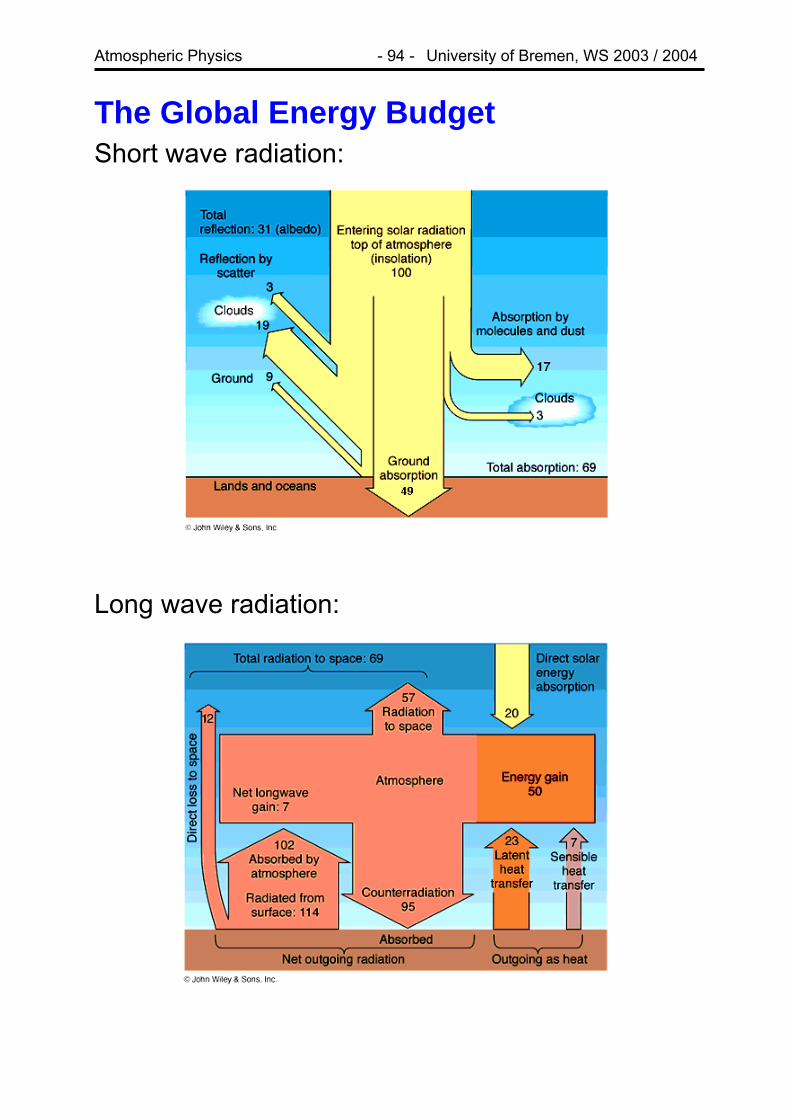
The Global Energy Budget Short wave radiation:
Long wave radiation:

Atmospheric Physics - 95 - University of Bremen, WS 2003 / 2004
All other energy inputs into the system are small in comparison:
process [W/m2]cosmic radiation 0.01 fossil fuels and nuclear energy 0.02 Geothermal energy 0.06 Heat storage in the ocean for a temperature increase of 0.3 K/century
0.2
Energy required for a complete melting of ice sheets in 1000 years
0.6
Thus, over longer time periods, earth is in radiative equilibrium with the sun. Incoming Solar radiation:
1368 (R2 π)/(4πR2) ≈ 345 W/m2. 30% is reflected, the remaining 70% are absorbed and re-emitted as thermal radiation.

Atmospheric Physics - 96 - University of Bremen, WS 2003 / 2004
Energy Transport The energy input is larger close to the equator than at the poles, and only through poleward transport of energy by ocean currents, air circulation and latent heat flux, balance is achieved:
A significant amount of energy is also transported from the surface vertically to the lower troposphere in the form of sensible and latent heat.

Atmospheric Physics - 97 - University of Bremen, WS 2003 / 2004
The Solar Spectrum
• black body of 5780K in first approximation • large deviations in the X-ray, far UV and
microwave region, where solar emission is many orders of magnitude larger than expected from a black body
• in these spectral regions, the emission is also highly variable and linked to sunspots, flares and the 11 year cycle
• total solar output is constant within a few percent

Atmospheric Physics - 98 - University of Bremen, WS 2003 / 2004
Penetration depth of solar radiation
• above 90 km, ionization of air molecules => ionosphere, thermosphere, very high temperatures at low density
• 100..200 nm: photodissociation of O2, formation of reactive O
• 200..310 nm: photodissociation of O3 in the ozone layer, stratosphere
• > 310 nm: depends strongly on cloud cover The energy balance of the upper atmosphere is to a large degree determined by the high energy part of the solar spectrum

Atmospheric Physics - 99 - University of Bremen, WS 2003 / 2004
Earth Radiation Budget from Space Several satellites have been deployed to measure the Earth’s radiation budget: • NASA’s Earth Radiation Budget Experiment
(ERBE) with instruments on Nimbus 6, Nimbus 7, and NOAA-9 and NOAA-10 from 1987 on
• Earth Radiation Budget Satellite (ERBS), launched from Space shuttle in 1984
• Scanner for Radiation Budget ScaRaB on Meteor 1994
• CERES (Clouds and the Earth's Radiant Energy System) on TRMM (2000)
• Geostationary Earth Radiation Budget instrument GERB on MeteoSat-2 2002
Basic idea: Direct measurements of shortwave and longwave outgoing and incoming radiation Problems: • very high absolute accuracy needed • spatial and temporal sampling must be
sufficient to exclude biases in the averages
Atmospheric Physics - 100 - University of Bremen, WS 2003 / 2004
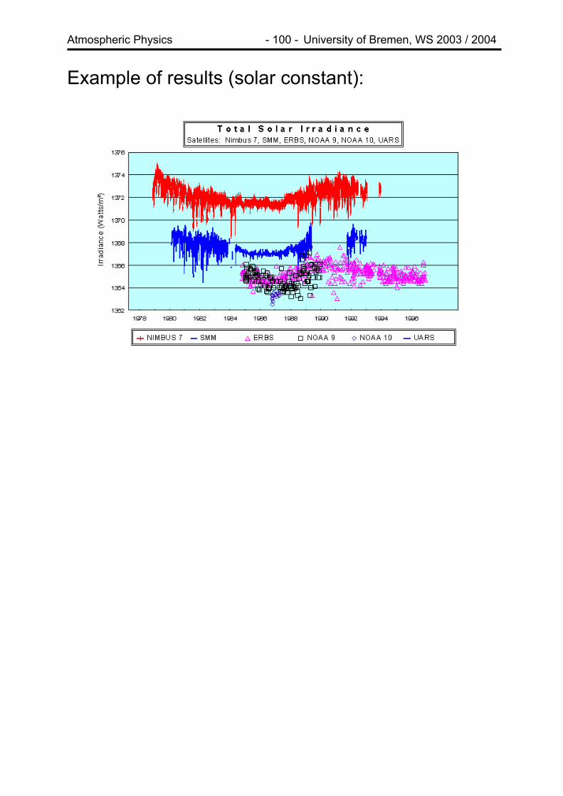
Example of results (solar constant):

Atmospheric Physics - 101 - University of Bremen, WS 2003 / 2004
Quantities Relevant for Climate Input parameters: • incoming radiation (solar activity, earth’s orbit) • concentrations of IR absorbing gases • concentrations of aerosols (volcanic eruptions) • surface albedo (ice and snow coverage) • cloud cover • ocean currents (salinity, sea ice)
Affected parameters • surface temperature • sea levels • cloud cover • precipitation • frequency of storms / droughts • ocean currents

Atmospheric Physics - 102 - University of Bremen, WS 2003 / 2004
IR Absorption by Molecules Depending on wavelength (= energy), different physical processes are responsible for absorption: UV dissociation VIS electronic transitions IR vibrational transitions MW rotational transitions In practice, combinations of the different processes occur leading to spectra with many lines (one vibration with several rotational transitions) To absorb in the IR, a molecule must • have more than one atom • have the right oscillation frequency • have a separation of charges (dipole moment)
to couple to the electromagnetic waves Molecules that do not absorb in the IR are • Ar (one atom) • N2, O2 (no dipole moment) • CO (symmetric stretch)

Atmospheric Physics - 103 - University of Bremen, WS 2003 / 2004
Molecules that do absorb in the IR are • CO2, H2O, CH4, N2O, CFCs
How efficient the IR absorption by a molecule is, depends on • concentration of the substance • atmospheric lifetime of the substance • absorption cross-section • position of absorption bands relative to those
of other absorbers Non-linearity of absorption: Absorption follows Lambert Beer’s law, and only for very small absorptions it depends linearly on the amount of the absorber. Therefore, absorbers are most effective in spectral regions, where no other absorbers are present (Atmospheric Windows) while in contrast adding more of an already strong absorber changes little in the radiative balance!
Atmospheric Physics - 104 - University of Bremen, WS 2003 / 2004
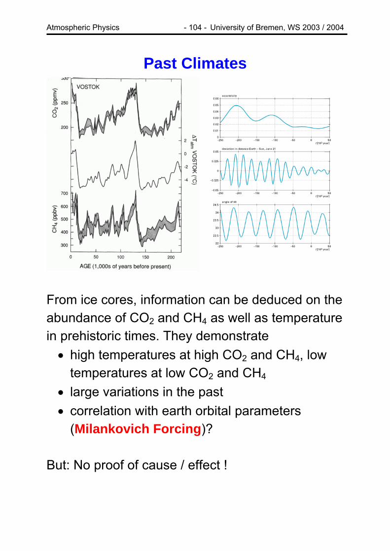
Past Climates
From ice cores, information can be deduced on the abundance of CO2 and CH4 as well as temperature in prehistoric times. They demonstrate • high temperatures at high CO2 and CH4, low
temperatures at low CO2 and CH4 • large variations in the past • correlation with earth orbital parameters
(Milankovich Forcing)? But: No proof of cause / effect !
Atmospheric Physics - 105 - University of Bremen, WS 2003 / 2004
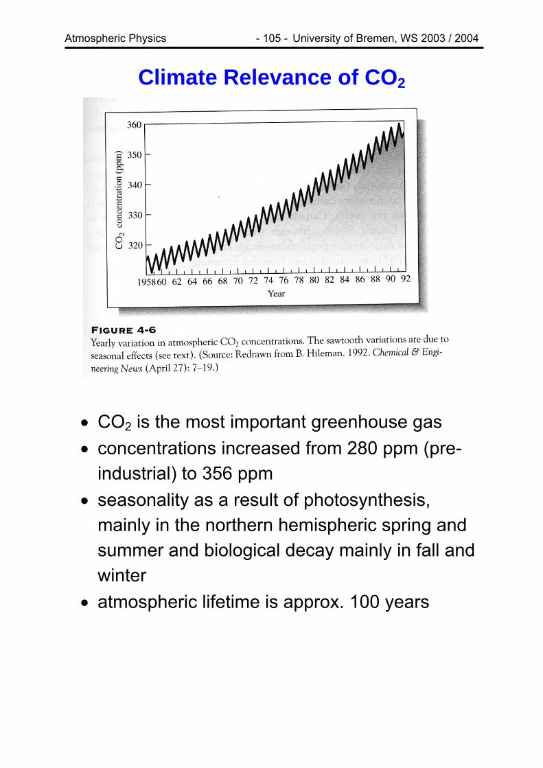
Climate Relevance of CO2
• CO2 is the most important greenhouse gas • concentrations increased from 280 ppm (pre-
industrial) to 356 ppm • seasonality as a result of photosynthesis,
mainly in the northern hemispheric spring and summer and biological decay mainly in fall and winter
• atmospheric lifetime is approx. 100 years

Atmospheric Physics - 106 - University of Bremen, WS 2003 / 2004
Anthropogenic Sources: • fossil fuel combustion and cement production
(75%) • biomass burning and deforestation (25%)
Sinks: • oceans (solution, calcium carbonate formation
and deposition) • forests in the northern hemisphere (growing)
Feedbacks: • photosynthesis is increased when more CO2 is
available (and often at higher temperature) → negative feedback
• solubility of CO2 in water is reduced when temperature increases → positive feedback

Atmospheric Physics - 107 - University of Bremen, WS 2003 / 2004
Climate Relevance of H2O • second most important greenhouse gas • often not explicitly named • per molecule, H2O is less effective than CO2
but much more abundant • concentrations vary strongly in space and time • relatively small anthropogenic influence
Feedbacks: • partial pressure of H2O increases exponentially
with temperature → positive feedback • cloud formation depends on H2O concentration
o high cirrus clouds warm → positive feedback
o low clouds cool → negative feedback o highly uncertain!

Atmospheric Physics - 108 - University of Bremen, WS 2003 / 2004
Climate Relevance of CH4
• CH4 concentrations doubled to 1.7 ppm today • currently, concentrations are stable for
unknown reasons • highly uncertain emissions • atmospheric lifetime is about 15 years
Sources: • wetlands • fossil fuel use (CH4 losses in gas transport can
offset advantage of using gas instead of coal!) • landfills • ruminants • rice paddies • forest clearing
Sinks: • reaction with OH • transport to stratosphere
Atmospheric Physics - 109 - University of Bremen, WS 2003 / 2004
Feedbacks: • change in CH4 could induce change in OH
concentration → negative feedback (possible reason for observed reduction in trend)
• increase in stratospheric H2O: O* + CH4 → OH + CH3 OH + CH4 → H2O + CH3 → positive feedback
• methane from permafrost regions might be released at higher temperatures → positive feedback
• methane (in methane hydrates CH4.6H2O) from
the ocean floors might be released at higher temperatures→ positive feedback
→ Runaway Greenhouse Effect possible but rather speculative

Atmospheric Physics - 110 - University of Bremen, WS 2003 / 2004
Climate Relevance of N2O • concentration roughly 0.31 ppm • growing 9% / year
Sources: • ocean • tropical soils • nitrification / denitrification in soils has N2O as
by-product • use of fertilizer • burning of N-containing fuels (coal, biomass) • older catalytic converters
Sinks: • stratosphere, photolysis
Feedbacks: • in the stratosphere, N2O is a source of NOx
which can lead to ozone destruction → negative feedback
Atmospheric Physics - 111 - University of Bremen, WS 2003 / 2004
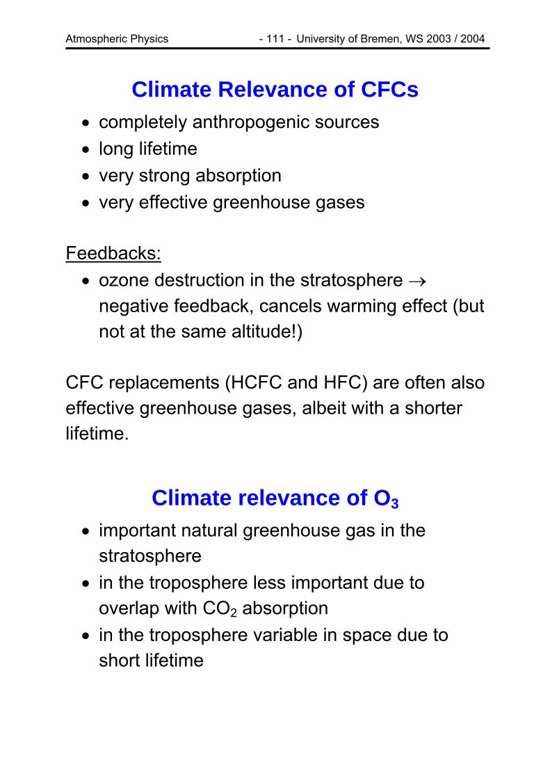
Climate Relevance of CFCs • completely anthropogenic sources • long lifetime • very strong absorption • very effective greenhouse gases
Feedbacks: • ozone destruction in the stratosphere →
negative feedback, cancels warming effect (but not at the same altitude!)
CFC replacements (HCFC and HFC) are often also effective greenhouse gases, albeit with a shorter lifetime.
Climate relevance of O3
• important natural greenhouse gas in the stratosphere
• in the troposphere less important due to overlap with CO2 absorption
• in the troposphere variable in space due to short lifetime

Atmospheric Physics - 112 - University of Bremen, WS 2003 / 2004
Climate Relevance of Aerosols • aerosols have a multitude of conflicting effects
on climate • sulphate aerosols mostly reflect solar light →
net cooling • soot mostly absorbs light → net warming • aerosols provide condensation nuclei that
affect o cloud formation o cloud droplet size → reflectivity (larger for
smaller droplets) • aerosols tend to cool in mid-latitudes and heat
at low latitudes, leading to changes in temperature gradients
• many feedbacks exist for aerosol deposition, cloud formation and increased aerosol production in drier climates
Sources: • sea-salt • soils • anthropogenic SO2 emissions • DMS emissions

Atmospheric Physics - 113 - University of Bremen, WS 2003 / 2004
Quantification of Climate Relevance The climate relevance of a species is often given as the Radiative Forcing = net change in radiative energy flux at the tropopause to changes in the concentration of a given trace gas To simplify calculations, everything is given relative to the effect of CO2: Effective Carbon Dioxide Concentration = concentration of CO2 that leads to same change in surface temperature Often, Indirect Effects are also important and much more difficult to quantify:

Atmospheric Physics - 114 - University of Bremen, WS 2003 / 2004
Global Warming Potentials
For each substance, a Global Warming Potential is computed, that gives the time integrated change of radiative forcing due to the instantaneous release of 1 kg of a trace gas relative to the effect of the release of 1 kg CO2
The global warming potential depends on the time interval treated and also on many other assumptions!
Atmospheric Physics - 115 - University of Bremen, WS 2003 / 2004
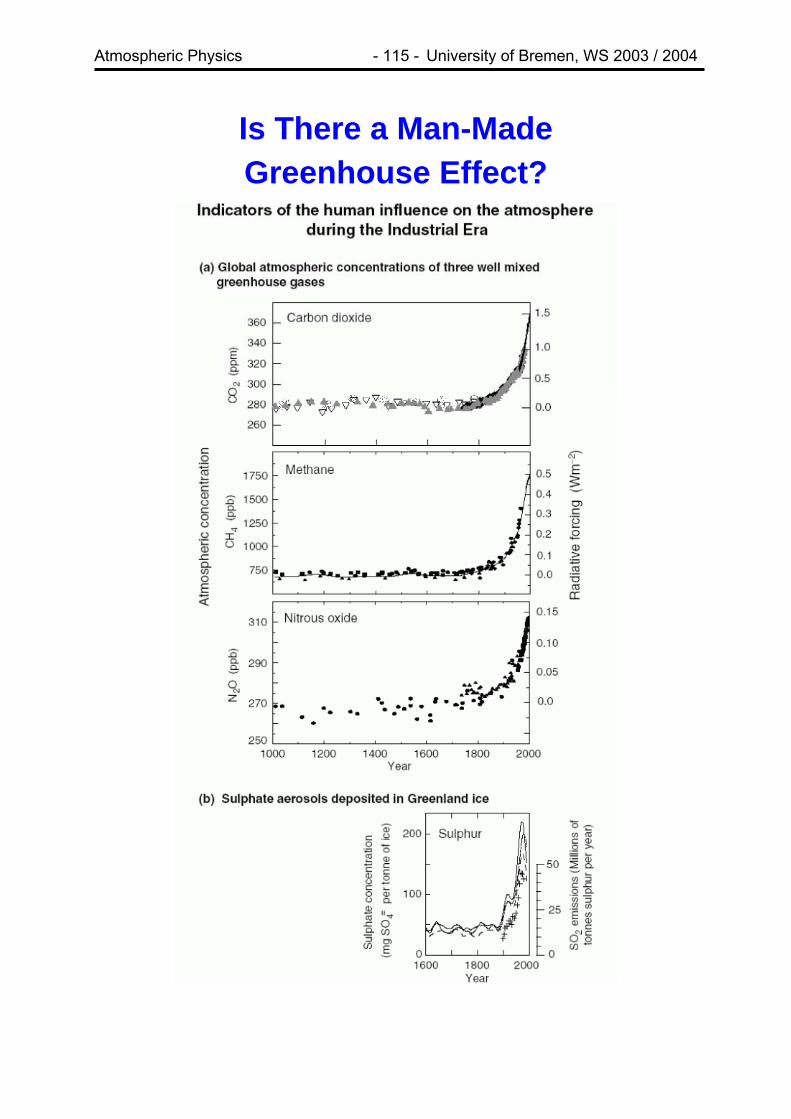
Is There a Man-Made Greenhouse Effect?

Atmospheric Physics - 116 - University of Bremen, WS 2003 / 2004
Is Temperature Changing on Earth?

Atmospheric Physics - 117 - University of Bremen, WS 2003 / 2004
What are the Main Contributions to GW?
• many contributions are still not well quantified • in particular aerosol effects are very uncertain • the impact of CO2 and CH4 is well understood

Atmospheric Physics - 118 - University of Bremen, WS 2003 / 2004
How well do Models?
• models can qualitatively reproduce past temperature changes
• climate models still are rather simplistic • chemistry is not well represented in climate
models, which might have a big impact on the predictions
• input for models is still rather uncertain

Atmospheric Physics - 119 - University of Bremen, WS 2003 / 2004
What do Models Predict?

Atmospheric Physics - 120 - University of Bremen, WS 2003 / 2004
Summary Greenhouse Effect • the natural greenhouse effect is crucial for the
current moderate temperatures at the Earth surface
• the concentration of many greenhouse gases in the atmosphere increases as a result of human activities
• eventually, larger concentrations of CO2 and others will increase temperatures on Earth
• temperature on Earth has already increased significantly in the last 100 years
• it is probable but not sure that the increase in greenhouse gases is the (only) reason for the observed increase in temperature
• many feedback processes make quantitative predictions difficult
• in particular aerosols play different roles in the climate system and can lead to both warming and cooling depending on conditions
Atmospheric Physics - 121 - University of Bremen, WS 2003 / 2004
Work, Heat and Energy A system is a part of the world in which we have a special interest, such as a reaction vessel or an air parcel. The energy of a system can be changed by doing (mechanical) work on it; in the atmosphere this is done by changing the volume. The energy of a system can also be changed by transferring heat as a result of a temperature difference between system and surroundings. A change in state of the system that is performed without heat being transferred is called adiabatic. A process that releases energy is exothermic, a process that absorbs energy is called endothermic. By convention, energy supplied to a system is written positive, energy that has left the system is negative.

Atmospheric Physics - 122 - University of Bremen, WS 2003 / 2004
Energy and Enthalpy The Internal Energy U is the total energy of a system. A change in internal energy of a system is the sum of the changes of energy through work dW and heat dQ :
pdVTdSdWdQdU −=+= For a system with constant volume, no mechanical work is performed and the change in internal energy equals the transferred heat:
VdQdU =
The Enthalpy of a system is defined as H = U + pV.
At constant pressure, a change in enthalpy equals the transferred heat:
pdQdH =
Internal Energy and Enthalpy are State Functions that depend only on the state of the system and not on the way how it was achieved. This is not true for Q and W!

Atmospheric Physics - 123 - University of Bremen, WS 2003 / 2004
Entropy The internal energy U is a state function that lets us assess if a process is permissible, the Entropy S is a state function that tells us, which processes proceed spontaneously. The statistical definition of Entropy S is
S = k ln W where k is Boltzmann’s constant and W the number of possible states of the system giving the same energy. The thermodynamic definition of an Entropy change dS is
TdQdS =
where dQ is the transfer of heat taking place at temperature T. Both definitions are identical. In general, only processes can occur that lead to an overall increase in entropy in system and surroundings.

Atmospheric Physics - 124 - University of Bremen, WS 2003 / 2004
Heat Capacities The heat capacity C of a system is the amount of heat Q needed to change the temperature T of a system: CdTdQ = .
The heat capacity of a system depends on the conditions: The heat capacity at constant volume CV is related to the change in internal energy U:
VV T
UC ⎟⎠⎞
⎜⎝⎛∂∂
=
The heat capacity at constant pressure Cp is related to the change in enthalpy H:
pp T
HC ⎟⎠⎞
⎜⎝⎛∂∂
=
At constant pressure, work is performed by the system during heating, and therefore
CP > CV
For an ideal gas, nRCC vp =−

Atmospheric Physics - 125 - University of Bremen, WS 2003 / 2004
Laws of Thermodynamics 0th law: If A is in thermal equilibrium with B, and B is in thermal equilibrium with C, then C is also in thermal equilibrium with A. 1st law: The internal energy U of a system is constant unless it is changed by doing work (W) or by heating (Q):
WQU +=∆ 2nd law: The entropy S of an isolated system increases in the course of a spontaneous change:
0>∆ totS 3rd law: The entropy change of a transformation approaches zero as the temperature approaches zero:
0 as 0 →→∆ TS
Atmospheric Physics - 126 - University of Bremen, WS 2003 / 2004
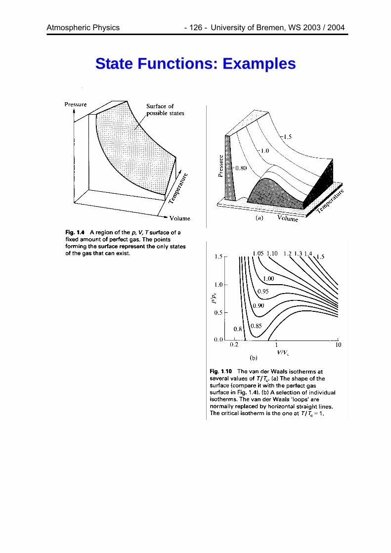
State Functions: Examples

Atmospheric Physics - 127 - University of Bremen, WS 2003 / 2004
Phase Changes An ideal gas is a gas independent of pressure and temperature. In real gases, however, forces between the molecules and also the finite volume of the individual molecules result in phase changes at certain temperatures and pressures. If a liquid is heated its temperature increases according to its heat capacity. However, if the boiling temperature is reached, further energy input does not result in increased temperature but only in more evaporation until the whole liquid has changed its phase. The energy needed to melt ice or evaporate a liquid is called latent heat. It can be recovered during condensation or sublimation.
Atmospheric Physics - 128 - University of Bremen, WS 2003 / 2004
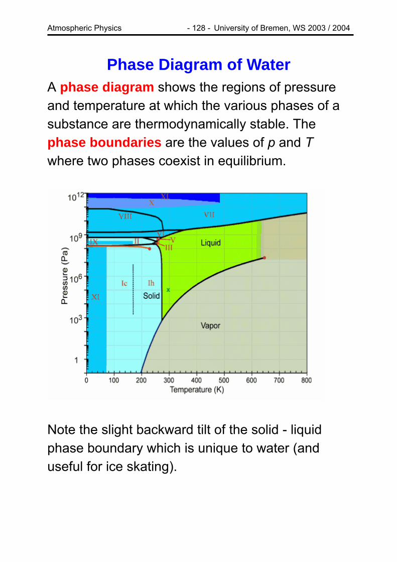
Phase Diagram of Water A phase diagram shows the regions of pressure and temperature at which the various phases of a substance are thermodynamically stable. The phase boundaries are the values of p and T where two phases coexist in equilibrium.
Note the slight backward tilt of the solid - liquid phase boundary which is unique to water (and useful for ice skating).

Atmospheric Physics - 129 - University of Bremen, WS 2003 / 2004
Water in the Atmosphere The amount of water in a given air volume is crucial for its ability to transfer energy. Common moisture parameters are:
mass mixing ratio: d
vmmw = where mv is the mass
of water vapour and md the mass of dry air saturation vapour pressure: the vapour pressure that is reached in equilibrium above a plane surface of pure water es or over ice esi. Note that es and esi depend only on temperature and that es > esi at all temperatures.
relative humidity: sw
wRH 100=
dew point: Temperature at which water vapour in a given air volume would start to condensate frost point: Temperature at which water vapour in a given volume would start to freeze
Atmospheric Physics - 130 - University of Bremen, WS 2003 / 2004
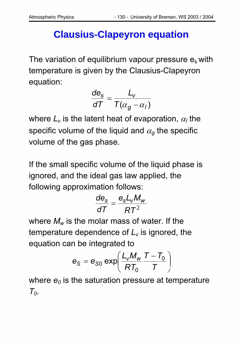
Clausius-Clapeyron equation The variation of equilibrium vapour pressure es with temperature is given by the Clausius-Clapeyron equation:
)( lg
vsT
LdTde
αα −=
where Lv is the latent heat of evaporation, αl the specific volume of the liquid and αg the specific volume of the gas phase. If the small specific volume of the liquid phase is ignored, and the ideal gas law applied, the following approximation follows:
2RTMLe
dTde wvss =
where Mw is the molar mass of water. If the temperature dependence of Lv is ignored, the equation can be integrated to
⎟⎟⎠
⎞⎜⎜⎝
⎛ −=
TTT
RTMLee wv
SS0
00 exp
where e0 is the saturation pressure at temperature T0.

Atmospheric Physics - 131 - University of Bremen, WS 2003 / 2004
Water Saturation Pressure
• water saturation pressure is an exponential
function of temperature • small changes in temperature have a large
effect on the amount of water that can be present as water vapour
Every day’s examples: • dry air in heated rooms • “fogging” of glasses • white plumes above chimneys
Atmospheric Physics - 132 - University of Bremen, WS 2003 / 2004
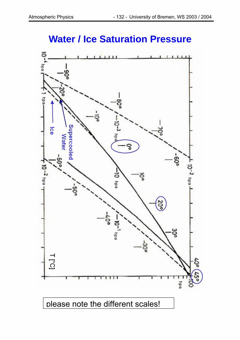
Water / Ice Saturation Pressure
!
please note the different scales
Atmospheric Physics - 133 - University of Bremen, WS 2003 / 2004
Latent Heat
The energy needed to evaporate 1 kg of water is about three times as large as the energy needed to heat it from 0°C to 100°C!

Atmospheric Physics - 134 - University of Bremen, WS 2003 / 2004
Water Vapour Measurements Hair Hygrometer: Length of a human hair or other fine thread is expanding in moist air Semiconductor Hygrometer: Some semiconductors change resistance as a function of humidity Frost Point Hygrometer: A mirror is cooled and the temperature at which it is fogged by condensation / frost is recorded:
Psychrometer: A wet and dry bulb thermometer measure the temperature difference between a wet and a dry thermometer, which depends on air humidity Absorption Measurements
Atmospheric Physics - 135 - University of Bremen, WS 2003 / 2004
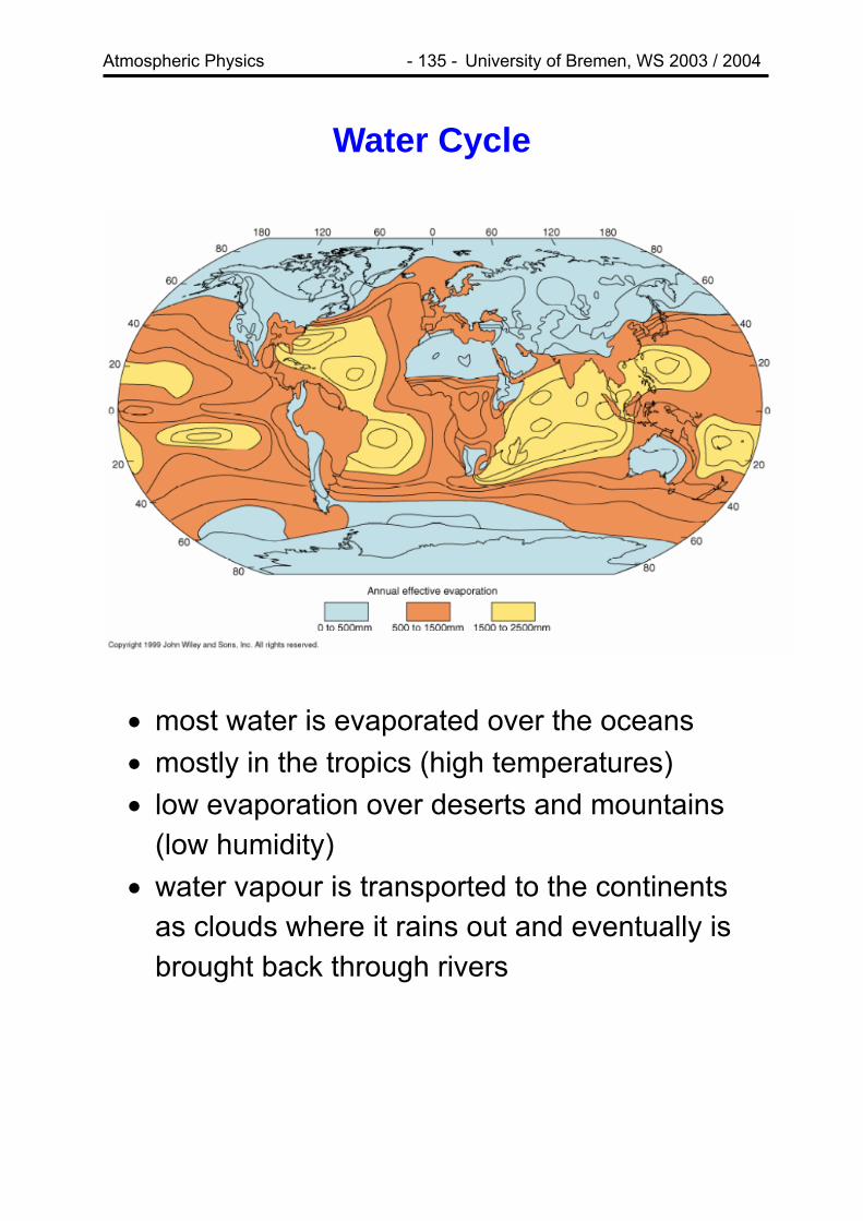
Water Cycle
• most water is evaporated over the oceans • mostly in the tropics (high temperatures) • low evaporation over deserts and mountains
(low humidity) • water vapour is transported to the continents
as clouds where it rains out and eventually is brought back through rivers
Atmospheric Physics - 136 - University of Bremen, WS 2003 / 2004
Air Parcels Mixing in the atmosphere can be obtained by two types of processes: molecular diffusion: small scale (< 1cm) and in the upper atmosphere turbulent and convective mixing: dominant below 100 km In turbulent and convective mixing, one imagines “air parcels” to be moved around, which have dimensions of several meters up to 1000 km (horizontally). Air parcels are by definition • thermally well insulated (adiabatic processes) • have always the same pressure as the
environment • have negligible kinetic energy (Uint >> Ekin)
Although these conditions are usually not all fulfilled, air parcels still prove to be a useful concept.

Atmospheric Physics - 137 - University of Bremen, WS 2003 / 2004
Cooling or Warming at Constant p
• cooling an air parcel isobarically from R to Q
will increase the relative humidity as es decreases
• further cooling will lead to condensation (fog formation) and a reduced cooling rate
• this is the explanation for “radiation fog” that forms close to the surface that loses energy through radiation at night under cloud free conditions
Atmospheric Physics - 138 - University of Bremen, WS 2003 / 2004
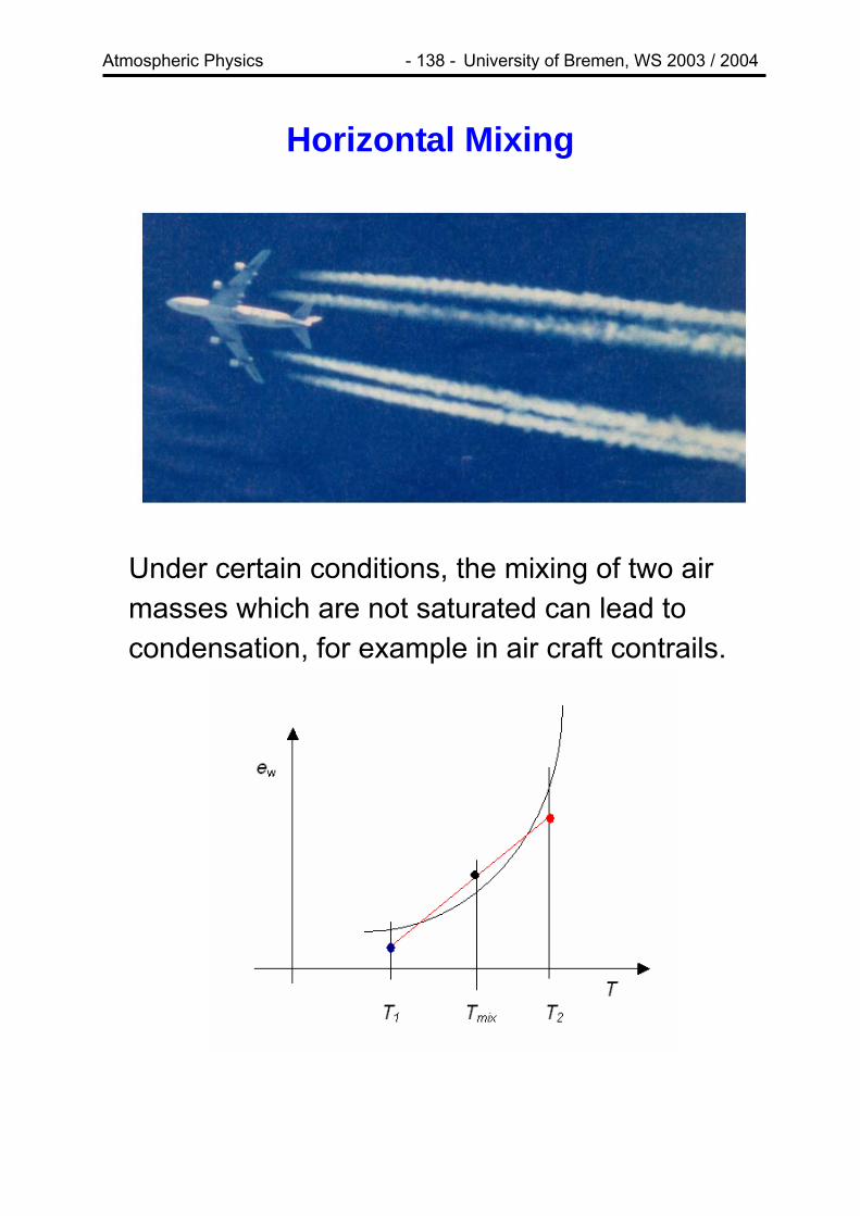
Horizontal Mixing
Under certain conditions, the mixing of two air masses which are not saturated can lead to condensation, for example in air craft contrails.

Atmospheric Physics - 139 - University of Bremen, WS 2003 / 2004
Adiabatic Expansion / Compression
When moving an air parcel vertically in the atmosphere, one can assume that no heat is exchanged with the surroundings (adiabatic). How is the temperature changing in such a process? First Law:
dTCdUpdVdQdWdQdU
V=−=+=
Adiabatic: pdVdTCdQ V −=→= 0
Ideal gas law (1 mole): RdTpdVVdpRTpV =+→=
Insert:
pdp
CR
TdT
dpp
RTdTC
VdpdTCVdpdTRCRdTVdpdTC
p
p
p
V
V
=
=
=
=+
−=
)(

Atmospheric Physics - 140 - University of Bremen, WS 2003 / 2004
By integrating we find the Poisson equation:
Vp
CR
CR
CRp
p
p p
T
T
ccconstpT
pTTp
pp
TT
pp
CR
TT
pdp
CR
TdT
pp
p
/
lnln
==
=
⎟⎟⎠
⎞⎜⎜⎝
⎛=
⎟⎟⎠
⎞⎜⎜⎝
⎛=⎟⎟
⎠
⎞⎜⎜⎝
⎛
=
−
−−
∫∫
κκ
κ
1
00
00
00
00
From the hydrostatic equation, we know that
dzRTMg
pdp
−=
Thus
dzRTMgdT
RTCp −=
and finally the adiabatic lapse rate
pCMg
dzdT
−==Γ

Atmospheric Physics - 141 - University of Bremen, WS 2003 / 2004
For dry air, the adiabatic lapse rate is approximately
mKMolJK
msgMoldzdT 100/1
97.2881.997.28
11
21−≈−=
−−
−−
Potential Temperature Starting from the adiabatic lapse rate, a new temperature can be defined that is the temperature an air parcel would have if brought adiabatically to p0=1013 mbar. The potential temperature Θ can be derived using the Poisson equation:
10
1 −−Θ
== κ
κ
κ
κ
pconst
pT
Potential Temperature: κ
κ 1
0
−
⎟⎠
⎞⎜⎝
⎛=ΘppT
The potential temperature is a measure of the sum of potential and internal energy and often a conserved quantity. ((κ -1) / κ = 0.286 in air)
Atmospheric Physics - 142 - University of Bremen, WS 2003 / 2004
Pseudoadiabatic Lapse Rate When considering humid air (no condensation), the change in heat capacity must be considered, but the effect is very small (see exercises), Things change significantly, if moist air is treated, and condensation takes place. Latent heat released during condensation is increasing the temperature and thereby reduces the temperature gradient. In contrast to the dry case, dQ is not zero but equals the amount of released latent heat Lv:
MgdzdTCdQ
dpp
RTdTCdQ
p
p
+=
−=
As condensation depends only on the number of moles water vapour, we multiply with n/V=p/RT:
svp wdLdz
RTMgpdT
RTpC
dQ −=+=
where sdw is the absolute humidity at saturation pressure.

Atmospheric Physics - 143 - University of Bremen, WS 2003 / 2004
As sdw is a function of temperature,
dTdTwdLdz
RTMgpdT
RTpC s
vp −=+
and finally the pseudoadiabatic lapse rate is
dTwdRTLpC
MpgdzdT
svp +
−=
The water saturation mixing ratio ws is linked to the water saturation pressure which can be determined using the Clausius-Clapeyron equation. The pseudoadiabatic lapse rate is always smaller than the adiabatic lapse rate. How much it differs from the adiabatic lapse rate depends on temperature; at high temperatures, the difference increases. At low temperatures (0..5°C) a typical value is 0.5K/100m.

Atmospheric Physics - 144 - University of Bremen, WS 2003 / 2004
Pseudoadiabatic Chart
black solid: dry adiabats (constant Θ) red solid: water saturation red dashed: pseudoadiabats

Atmospheric Physics - 145 - University of Bremen, WS 2003 / 2004
Stability If a dry air parcel is moved vertically in an atmosphere with an adiabatic lapse rate, its temperature (and thus density) will always be the same as that of its environment (neutral situation). If the actual lapse rate γ is smaller than the adiabatic lapse rate Γ (T decreasing less with altitude), a parcel lifted will be colder than its environment, which means it is denser and heavier leading to a downward force (stable situation). If, however, the lapse rate γ in the atmosphere is larger than Γ (T decreasing more rapidly with height), then Tparcel > Tenviro when the parcel is lifted, and thus the density is smaller, leading to an upwards force (unstable situation)
-γ < -Γ stable Please note the sign convention that might differ in other texts!
-γ = -Γ neutral
-γ >- Γ unstable As the pseudoadiabatic lapse rate is smaller than Γ, a lapse rate that is stable for dry air can be

Atmospheric Physics - 146 - University of Bremen, WS 2003 / 2004
unstable for moist air! To assess the importance of this effect, one can evaluate the equivalent temperature, which is the temperature an air parcel would have if all latent heat would be converted to heat:
p
ve C
LwTT +=
Te can be much larger than T and thus at large w air parcels can rise high even in stable situations.
Inversions If the temperature actually increases with altitude (temperature inversion), the atmosphere is particularly stable and water vapour, aerosols, and pollutants are trapped: • positive feed back through fog formation • important for local pollution • often occurring in high pressure situations
when air subsides adiabatically • particularly persistent in valleys • boundary layer inversion through accumulation
of water vapour and aerosols close to the surface
• nightly inversion through radiative cooling
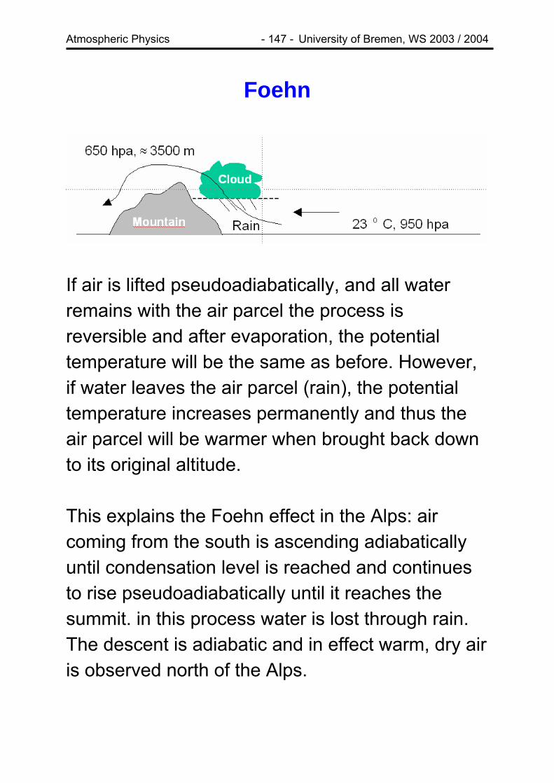
Atmospheric Physics - 147 - University of Bremen, WS 2003 / 2004
Foehn
If air is lifted pseudoadiabatically, and all water remains with the air parcel the process is reversible and after evaporation, the potential temperature will be the same as before. However, if water leaves the air parcel (rain), the potential temperature increases permanently and thus the air parcel will be warmer when brought back down to its original altitude. This explains the Foehn effect in the Alps: air coming from the south is ascending adiabatically until condensation level is reached and continues to rise pseudoadiabatically until it reaches the summit. in this process water is lost through rain. The descent is adiabatic and in effect warm, dry air is observed north of the Alps.

Atmospheric Physics - 148 - University of Bremen, WS 2003 / 2004
Lee (Gravity) Waves
In the lee of mountains, gravity or lee waves form that sometimes can be observed as periodic cloud fields extending long distances after the mountain. We evaluate the force F acting on the air parcel (*) when it is displaced adiabatically from the equilibrium by *
0T zδ :
*)(* ρρδρ −== gFdt
zd2
2
with ρ ∝ 1/T we find
TTTg
TTTg
dtzd −
=−
=*
*/*//
111
2
2δ
The temperature of the air parcel changes adiabatically
zTzT δΓ+= *)(* 0

Atmospheric Physics - 149 - University of Bremen, WS 2003 / 2004
while the temperature of the surroundings changes with
zTzT γδ+= 0)( Thus the temperature difference is
zzTzT δγ )()()(* −Γ=− and the vertical acceleration
zT
gdt
zd δγδ −Γ=2
2
which is the differential equation of a harmonic oscillator:
02
2=
Γ−+ z
Tg
dtzd δγδ
The solution is a sinusoidal oscillation with a period Tg of
( )Γ−=
γπ
Tg
Tg12
or a frequency gg T/1=ν of
( )Γ−= γπ
νTg
g 21
This frequency is called the Brunt- Väisälä frequency. Lee waves form, if the time the air needs to flow around the mountain is similar to Tg.

Atmospheric Physics - 150 - University of Bremen, WS 2003 / 2004
Thunderstorm Clouds
(a) cumulus state • warm, rising air • updraft velocities increase with height • top of cloud moves upwards • super cooled raindrops in cloud
(b) mature state • downward circulation of ice crystals, heavy rain • super cooled rain drops above freezing level,
snow and hail below • top of cloud reaches tropopause, anvil forms
(c) dissipating state • precipitation throughout the cloud • no updraft • no new drop formation
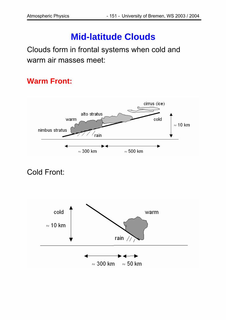
Atmospheric Physics - 151 - University of Bremen, WS 2003 / 2004
Mid-latitude Clouds Clouds form in frontal systems when cold and warm air masses meet: Warm Front:
Cold Front:

Atmospheric Physics - 152 - University of Bremen, WS 2003 / 2004
Cold Front
Cirrus
Stratocum

Atmospheric Physics - 153 - University of Bremen, WS 2003 / 2004
Clouds in the Upper Atmosphere Polar Stratospheric clouds (PSC): • form in the polar stratosphere • important for
chemistry (ozone hole)
• consist of ice, HNO3 and H2SO4
Noctilucent Clouds (NLC):
• form in upper mesosphere (> 80 km)
• polar summer • consist of ice

Atmospheric Physics - 154 - University of Bremen, WS 2003 / 2004
Condensation Condensation takes place if the saturation water vapour pressure decreases below the actual water vapour pressure in an air parcel. In the atmosphere, this usually happens through isobaric cooling or adiabatic ascent. In the absence of particles, condensation proceeds directly from the gas to the liquid phase (homogeneous condensation) starting on randomly formed micro-droplets. Homogeneous condensation is rare in the atmosphere as large supersaturations are needed over small droplets. If wettable or water soluble aerosol particles are present, they act as cloud condensation nuclei and overcome the problem of small droplets (heterogeneous condensation). If the aerosol is soluble, the saturation vapour pressure is further decreased and drop growth facilitated.
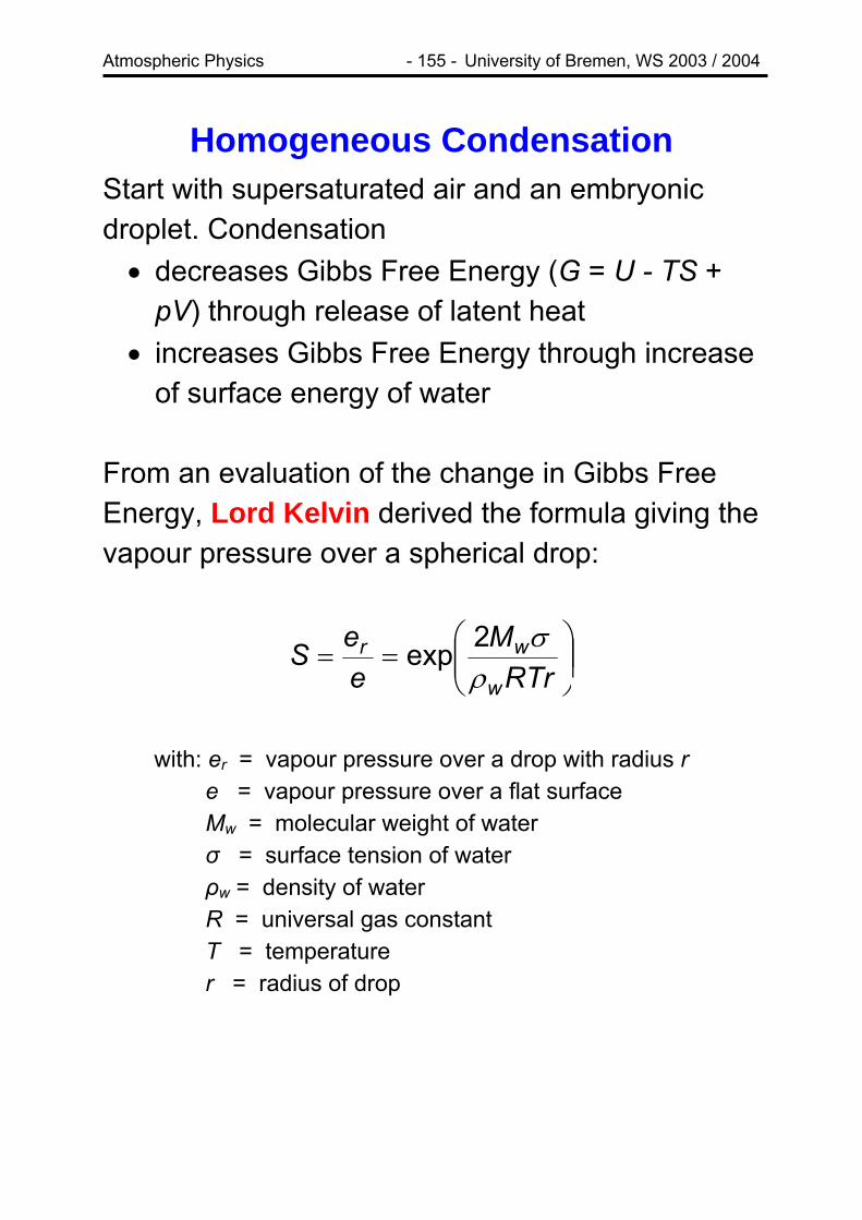
Atmospheric Physics - 155 - University of Bremen, WS 2003 / 2004
Homogeneous Condensation Start with supersaturated air and an embryonic droplet. Condensation • decreases Gibbs Free Energy (G = U - TS +
pV) through release of latent heat • increases Gibbs Free Energy through increase
of surface energy of water From an evaluation of the change in Gibbs Free Energy, Lord Kelvin derived the formula giving the vapour pressure over a spherical drop:
⎟⎟⎠
⎞⎜⎜⎝
⎛==
RTrM
eeS
w
wrρ
σ2exp
with: er = vapour pressure over a drop with radius r
e = vapour pressure over a flat surface Mw = molecular weight of water σ = surface tension of water ρw = density of water R = universal gas constant T = temperature r = radius of drop

Atmospheric Physics - 156 - University of Bremen, WS 2003 / 2004
Droplet growth is only possible if the supersaturation over the drop is at least Ses.. For a given supersaturation S*, a critical radius r* can be determined above which droplet growth takes place:
⎟⎟⎠
⎞⎜⎜⎝
⎛= *ln
2*SR
Mrw
w
ρσ
The values given in the table show, that typical supersaturations of a few percent correspond to a critical radius that can not be reached by random aggregation of water vapour molecules:
S* r* [µm] Number of Molecules 1.01 0.115 2.1·108
1.1 0.012 2.4·105
2 1.65·10-3 630 10 4.46·10-4 17
=> without importance in the atmosphere!

Atmospheric Physics - 157 - University of Bremen, WS 2003 / 2004
Aerosols Sources: • combustion • gas to particle conversion (H2SO4) • wind blown dust / sand • pollens • sea salt
Atmospheric Relevance: • scattering (visibility) • cloud condensation nuclei (CCN) • climate
Atmospheric Concentrations: • 10 .. 107 cm-3, decreasing with altitude
Size: • 10-4 µm .. 102 µm
Sinks: • gravitational setting • precipitation (80 - 90%)

Atmospheric Physics - 158 - University of Bremen, WS 2003 / 2004
Size Distribution: Often follows a power law
( )β−= DC
DddNlog
with C the concentration, D the diameter and β in the range of 2 - 4:
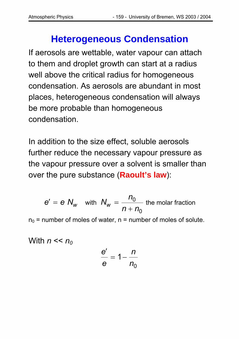
Atmospheric Physics - 159 - University of Bremen, WS 2003 / 2004
Heterogeneous Condensation If aerosols are wettable, water vapour can attach to them and droplet growth can start at a radius well above the critical radius for homogeneous condensation. As aerosols are abundant in most places, heterogeneous condensation will always be more probable than homogeneous condensation. In addition to the size effect, soluble aerosols further reduce the necessary vapour pressure as the vapour pressure over a solvent is smaller than over the pure substance (Raoult’s law):
wNee =′ with 0
0
nnnNw +
= the molar fraction
n0 = number of moles of water, n = number of moles of solute. With n << n0
01
nn
ee
−=′

Atmospheric Physics - 160 - University of Bremen, WS 2003 / 2004
Considering the dissociation efficiency i (i = 2 for NaCl)
⎟⎟⎠
⎞⎜⎜⎝
⎛=
s
sA M
mNin and ⎟⎟⎠
⎞⎜⎜⎝
⎛=
w
wA M
mNn0
NA = Avogadro number ms = mass of solute mw = mass of water
Ms = molecular weight of solute Mw = molecular weight of water
and approximating the density of the solution by that of pure water ρw
ww rm ρπ 3
34
=
we find for the vapour pressure over a solution
31
431
rMMmi
ee
sw
ws
ρπ−=
′
Combining Raoult’s with Kelvin’s law:
⎥⎦
⎤⎢⎣
⎡−⎟⎟
⎠
⎞⎜⎜⎝
⎛= 3
14312exp
rMMmi
RTrM
ee
sw
ws
w
rρπρ
σ

Atmospheric Physics - 161 - University of Bremen, WS 2003 / 2004
The combination of Raoult’s law and the Kelvin law leads to the Köhler curves:
For a given saturation, a small drop will increase according to the Köhler curve. If the saturation is above the maximum of the Köhler curve, the drop will continue to grow, else it will be stable (haze). A drop with a radius larger than the radius of the maximum of the Köhler curve (typically 0.1 - 1 µm) is called activated.

Atmospheric Physics - 162 - University of Bremen, WS 2003 / 2004
Example: • assume 3·10-16 g NaCl content in the droplet • water vapour pressure 0.6% below the
saturation over plane water • => final radius of the droplet ≈ 0.15 µm • if a supersaturation of 0.24% or more is
assumed, the droplet will grow to 0.2 µm where it has reached its critical radius and will continue to grow, this means the particle is activated.
The fraction of activated condensation nuclei is always small (≈ 200 cm-3) compared to the total number of nuclei which is several orders of magnitude larger.

Atmospheric Physics - 163 - University of Bremen, WS 2003 / 2004
Droplet Growth by Condensation As long as water vapour pressure in the air exceeds the vapour pressure close to the droplet, it can grow through condensation. However, latent heat is released close to the drop, increasing temperature and decreasing relative humidity. Thus, drop growth is slowed down depending on the efficiency of heat transport from the drop and the gradient in water vapour pressure:
( )
44444 344444 211
1
111
−
⎟⎠⎞
⎜⎝⎛ −⎟⎟⎠
⎞⎜⎜⎝
⎛+
−=
F
v
w
wv
w RTL
KTML
eDMRT
Srdt
drρρ
D = the diffusion coefficient K = heat conductivity of air Lv = molar heat of vaporization ρw = density of water
Thus, if F and S are assumed to be constant, droplet growth is inversely proportional to the radius.

Atmospheric Physics - 164 - University of Bremen, WS 2003 / 2004
Example: Assuming for ro = 1 µm, F = 1.0·10-2 s µm-2 , and S = 1.001 we can estimate the time required for the drop to reach a given radius is:
Radius r [µm] Time t [s] 5 120 10 500 20 2000
Thus, fast growing clouds such as Cumulus will have a droplet size spectrum different from that of slow growing clouds (Cumulonimbus):

Atmospheric Physics - 165 - University of Bremen, WS 2003 / 2004
Droplet Growth by Accretion Droplet growth by condensation would be much too slow for the formation of rain drops of the size of millimetres! Such large drops form by accretion when faster falling large drops incorporate slower falling small drops. Falling speeds are difficult to compute; empirical values are:
Drop radius r [µm]
falling velocity v [cm/s]
0.01 1 0.1 30 - 70 1.0 400 - 650 5.0 900 - 1000

Atmospheric Physics - 166 - University of Bremen, WS 2003 / 2004
A simple calculation of the mass increase based on geometrical considerations is given by
( ) EvVWrRdtdm
speedaldifferenticylinderofAera ⎟⎟⎟⎟
⎠
⎞
⎜⎜⎜⎜
⎝
⎛
−+= 32143421
2π
W = total water content of cloud (1g m-3) E = aerodynamics correction factor
E ≈ 1 for R > 20 µm but decreases rapidly for smaller droplets. Assuming spherical droplets and r <<R the size growth dR/dt can be calculated:

Atmospheric Physics - 167 - University of Bremen, WS 2003 / 2004
( )
WVdtdR
RrRrE
RmwithEvVWRr
dtdR
w
ww
ρ
ρπρ
41
111
341
41
2
32
=
≈⎟⎠⎞
⎜⎝⎛ +→<<=
=−⎟⎠⎞
⎜⎝⎛ −=
,
When comparing accretion and condensation efficiencies, the different radii at which they operate become clear:
Condensation increases the size of smaller droplets and tends to homogenize the droplet spectrum whereas accretion favours the largest drops and leads to a separation in the droplet spectrum.
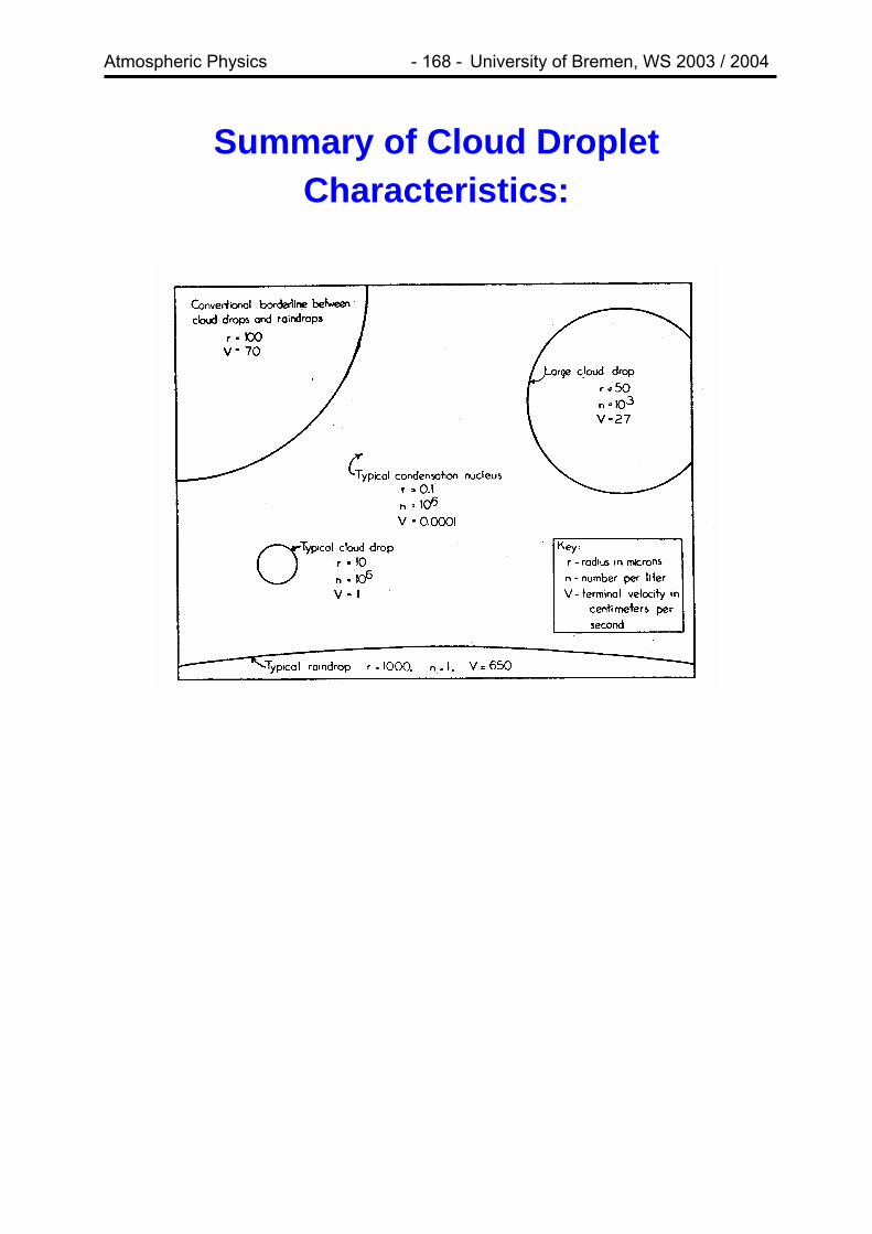
Atmospheric Physics - 168 - University of Bremen, WS 2003 / 2004
Summary of Cloud Droplet Characteristics:
Atmospheric Physics - 169 - University of Bremen, WS 2003 / 2004
Ice clouds / Findeisen Effect The situation for freezing is similar to that for condensation, and homogeneous nucleation is only realistic below a certain threshold temperature (≈ -36°C). Heterogeneous nucleation can occur at much higher temperatures if an appropriate freezing nucleus is available. The latter must have a molecular spacing and crystallographic arrangement similar to ice to be effective. As water saturation pressure is lower over ice than over water, ice particles will grow at the expense of supercooled water droplets (Findeisen Effect). Ice particles in clouds can grow by • growth from the vapour phase (Findeisen
Effect) => ice crystals • riming (freezing of supercooled droplets on a
falling ice particle) => hail • aggregation of ice particles
As a result of the geometry of ice particles, quantitative calculations of particle growth are difficult.
Atmospheric Physics - 170 - University of Bremen, WS 2003 / 2004
Overview over rest of winter term: Lecture: 7.1., 14.1., 21.1., 28.1.: Introduction to atmospheric dynamics 4.2.: Review of concepts Tutorial: 6.1. submit problems set 8 13.1. submit problems set 9 27.1. submit problems set 10 4.2. Review of concepts Exam: 16.2., 10:00 - 12:00 • only hand written notes • no copies / hand-outs / books • you will be supplied with
o table of constants and numerical values o pseudoadiabatic chart
Atmospheric Physics - 171 - University of Bremen, WS 2003 / 2004
Forces Acting on Air Parcels There are basically 4 different forces that act on a moving air parcel in the atmosphere: • gravitational force • pressure gradient force • Coriolis force (when parcel is moving) • frictional force (when parcel is moving)
There are also two distinct ways of looking at motion in the atmosphere: • Moving with the air parcel (Lagrangian
Description). In this description, the atmosphere is a collection of air parcels, all moving with individual velocities as a function of time. This is useful for detailed chemistry modelling and for the assessment of transport.
• Using a fixed coordinate system (Eulerian Description). Air properties are described as a function of location r
rand time t, for example
the velocity . The observer remains at the same position but air parcels will move by. This approach is useful for large scale models.
),( trvrr

Atmospheric Physics - 172 - University of Bremen, WS 2003 / 2004
Gravitational Force In first approximation, the gravitational force per volume acting on an air parcel is given by the gravitational acceleration and the mass of the air parcel:
gFgrr
ρ= ρ = density of air
gr = gravitational accelereation
To account for variations in gravitation with altitude and latitude we use the geopotential Φ and obtain
Φ−= gradρgF
r
It is important to note, that as a result of the horizontal inhomogeneity of the gravitational field, the gravitational force does not only have a vertical, but also a horizontal component.

Atmospheric Physics - 173 - University of Bremen, WS 2003 / 2004
Pressure Force In the presence of a pressure gradient, a force acts on an air parcel:
Assuming a pressure gradient in the x-direction, the effective force Fx is acting on the air parcel:
( )
xp
xAAp
VF
xAF
ApAppApF
xx
x
∂∂
−=−==
−=+−=
δδ
δ
δδ
Generalising this to the three dimensional case, we obtain for the pressure force per volume
pFp grad−=r

Atmospheric Physics - 174 - University of Bremen, WS 2003 / 2004
Coriolis Force In a rotating coordinate system, any moving mass that experiences an inertial force that is perpendicular both to the direction of movement and the axis of rotation. This Coriolis force, that is not observed in an inertial system is given per volume by
][2 Ω×=rrr
vFC ρ Ωr
= Earth angular velocity vr = velocity of air mass
A particle moving from P to A in an inertial system will follow a bent curve from P to A’ in the coordinate system of an observer on a rotating disc. He will explain this apparent acceleration by the Coriolis force.

Atmospheric Physics - 175 - University of Bremen, WS 2003 / 2004
Only the horizontal component of the Coriolis force is relevant in the atmosphere as • the vertical component is small compared to
the gravitational force • vertical speeds are small compared to
horizontal speeds • the vertical extension of the atmosphere, in
particular the troposphere is small Example: at v⊥ = 5 m/s and 1000 m vertical movement the Coriolis displacement is only about 20 m Thus, usually only the horizontal component of CF
r
is treated:
⊥Ω= vFC ρ2 ⊥Ω = vertical component of Earth angular velocity
v = horizontal velocity of air mass
Atmospheric Physics - 176 - University of Bremen, WS 2003 / 2004
The vertical component of the angular velocity is
ϕsinΩ=Ω⊥ with ϕ the latitude,
fvvFC ρϕρ =Ω= sin2 with ϕsin2Ω=f the Coriolis parameter. In vector notation and still assuming that there is only one component of the angular velocity
)sin,0,0( ϕΩ=Ω⊥r
we finally can write
][2 ⊥Ω×=rrr
vFC ρ • The Coriolis force is pointing to the right in the
Northern Hemisphere and to the left in the Southern Hemisphere.
• It is largest at the poles and 0 at the equator. • At the pole, the acceleration by the Coriolis
acceleration is of the order of 2vΩ =10-3m s-2
(5 m/s wind speed assumed) which is small compared to g but significant for large movements.

Atmospheric Physics - 177 - University of Bremen, WS 2003 / 2004
Frictional Force • Friction will occur within the atmosphere when
layers of air move at different velocities or at the ground.
• Friction on the surface depends very much on the surface type (water, desert, forest, ...).
• Friction between layers depends on the speed of momentum diffusion which can be both “thermal” diffusion and turbulent diffusion.
• Frictional forces are always directed against the direction of movement.
In first approximation, one can assume the frictional force per volume to be proportional to the speed:
vFFrr
κ−= κ = friction coefficient

Atmospheric Physics - 178 - University of Bremen, WS 2003 / 2004
Equation of Motion The equation of motion following from pressure gradient, gravitation, Coriolis force and friction is
FFvpdtvd rrrr
+Ω×+Φ−−= ][2gradgrad ρρρ
(unit volume, change in momentum equals sum of forces)
The left hand side can be separated in two parts:
• the change in local velocity with time tv∂∂r
• the change in velocity induced by the movement in space to a place where the velocity field has a different value (field
component) fielddt
vd⎟⎠⎞
⎜⎝⎛
r

Atmospheric Physics - 179 - University of Bremen, WS 2003 / 2004
The latter can for the x-direction be written as:
vvvz
vvyvv
xv
dtdz
zv
dtdy
yv
dtdx
xv
dtdv
xzx
yx
xx
xxx
field
x
r⋅=
∂∂
+∂∂
+∂∂
=
∂∂
+∂∂
+∂∂
=⎟⎠⎞
⎜⎝⎛
)(grad
or, in a formal notation
vvdtvd
field
rrr
)( ∇⋅=⎟⎠⎞
⎜⎝⎛
Using this notation, we have Euler’s equation of motion:
FFvpvvtv rrrrrr
+Ω×+Φ−−=∇⋅+∂∂ ][2gradgrad)( ρρρρ

Atmospheric Physics - 180 - University of Bremen, WS 2003 / 2004
Inertia Motion In the absence of external forces and friction, an air parcel moving at speed v0 in the atmosphere will not change is velocity. However, the Coriolis force will force it on a circular trajectory if the latitude dependence of Ω is neglected. In this simplest situation, the equation of motion is
0
20 fv
Rv
dtdv ρρρ ==
fvR 0=
R = radius of the motion The inertia radius R can give an indication for the scales at which the Coriolis force is important. At 5m/s, R varies from 35 km at the pole, 45 km at mid-latitudes and 130 km at 15° latitude. The time period needed for one complete inertia circle is 12h at the pole and 19h at mid-latitudes. It does not depend on v0 and R.

Atmospheric Physics - 181 - University of Bremen, WS 2003 / 2004
Geostrophic Wind In a slightly less simplified treatment we can look at the situation where friction can be neglected (altitude > 1000 m), and the gravitational acceleration is also ignored. The remaining forces are pressure gradient force and Coriolis force. The pressure gradient induces an acceleration from high to low pressure, but as the flow accelerates, it is diverted by the growing Coriolis force until the pressure gradient force (PGF) and the Coriolis force balance.
http://www.newmediastudio.org/DataDiscovery/Hurr_ED_Center/Easterly_%20Waves/Geostrophic_Wind/Geostrophic_Wind.html

Atmospheric Physics - 182 - University of Bremen, WS 2003 / 2004
Pressure changes in the atmosphere develop by different heating or cooling, topography, or air movements. They can be either large scale band structures or localized high / low pressure systems. In the stationary state, the PGF and Coriolis force have identical magnitude but opposite sign:
pv
FF
g
pC
grad][2 =Ω×
−=rr
rr
ρ
or written for the components
0
0
=∂∂
−−
=∂∂
−
ypvf
xpvf
gx
gy
ρ
ρ
yielding for the geostrophic wind vector gvr :
⎟⎟⎟⎟
⎠
⎞
⎜⎜⎜⎜
⎝
⎛
∂∂∂∂
−=
xp
f
yp
fvg
ρ
ρ1
1r
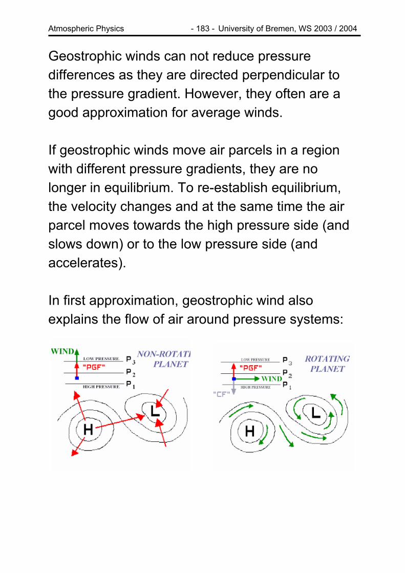
Atmospheric Physics - 183 - University of Bremen, WS 2003 / 2004
Geostrophic winds can not reduce pressure differences as they are directed perpendicular to the pressure gradient. However, they often are a good approximation for average winds. If geostrophic winds move air parcels in a region with different pressure gradients, they are no longer in equilibrium. To re-establish equilibrium, the velocity changes and at the same time the air parcel moves towards the high pressure side (and slows down) or to the low pressure side (and accelerates). In first approximation, geostrophic wind also explains the flow of air around pressure systems:

Atmospheric Physics - 184 - University of Bremen, WS 2003 / 2004
Examples in the Atmosphere

Atmospheric Physics - 185 - University of Bremen, WS 2003 / 2004
Ekman Spiral If friction at the surface is taken into account, the wind velocity decreases towards the surface and therefore also the direction of the flow changes from the geostrophic direction in the free troposphere to the surface wind direction. Thus, the wind vector describes a spiral, the Eckman spiral.
The angle between surface and geostrophic wind depends on surface roughness and is between 10° (smooth surface) to 50° (forests, cities).
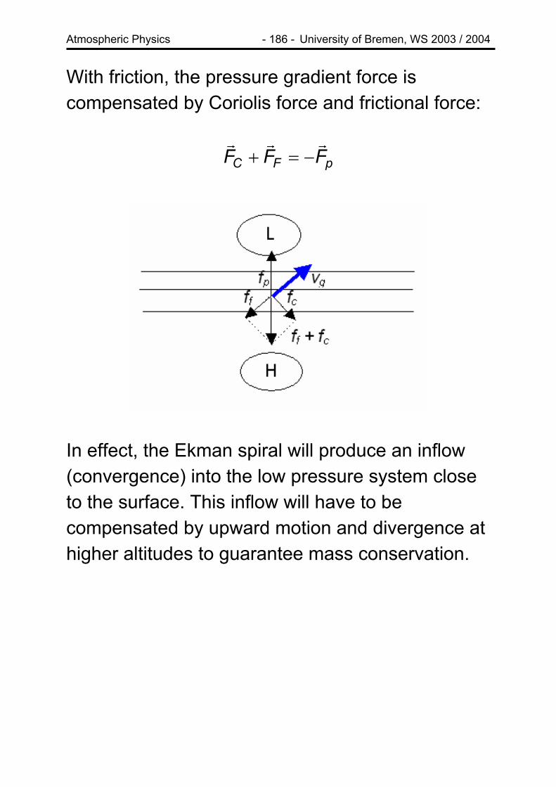
Atmospheric Physics - 186 - University of Bremen, WS 2003 / 2004
With friction, the pressure gradient force is compensated by Coriolis force and frictional force:
pFC FFFrrr
−=+
In effect, the Ekman spiral will produce an inflow (convergence) into the low pressure system close to the surface. This inflow will have to be compensated by upward motion and divergence at higher altitudes to guarantee mass conservation.
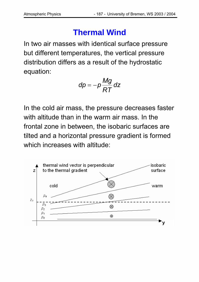
Atmospheric Physics - 187 - University of Bremen, WS 2003 / 2004
Thermal Wind In two air masses with identical surface pressure but different temperatures, the vertical pressure distribution differs as a result of the hydrostatic equation:
dzRTMgpdp −=
In the cold air mass, the pressure decreases faster with altitude than in the warm air mass. In the frontal zone in between, the isobaric surfaces are tilted and a horizontal pressure gradient is formed which increases with altitude:
y

Atmospheric Physics - 188 - University of Bremen, WS 2003 / 2004
As a result of the pressure gradient, a geostrophic wind forms which is again pointed to the right in the Northern Hemisphere and which increases with altitude as the gradient increases. Assuming a temperature gradient in the y-direction
⎟⎠⎞
⎜⎝⎛ <∂∂ 0YT , the flow will be in the x-direction, and the
change in vertical wind speed can be related to the temperature gradient at the surface: Hydrostatic equation:
RTMg
zp
RTMgp
gzp
−=∂
∂
−=
−=∂∂
ln
ρ
Geostrophic wind:
x
x
x
vRTMf
yp
vRTMfp
vfyp
−=∂∂
−=
−=∂∂
ln
ρ
Atmospheric Physics - 189 - University of Bremen, WS 2003 / 2004
Differentiating again and equating the second derivatives:
zTv
RMf
yT
RTMg
zyp x
∂∂
−=∂∂
=∂∂
∂ )/(ln2
2
yT
fTg
zTvx
∂∂
=∂
∂2
)/(
Approximating T by Tm, the mean temperature, we finally obtain
yT
fTg
zv m
m
x∂∂
=∂∂
Thus, if the temperature gradient is known and the velocity at one height, then the vertical profile of velocity can be calculated. The concept of thermal winds will be used to explain wind systems in mid-latitudes and also stratospheric wind systems.
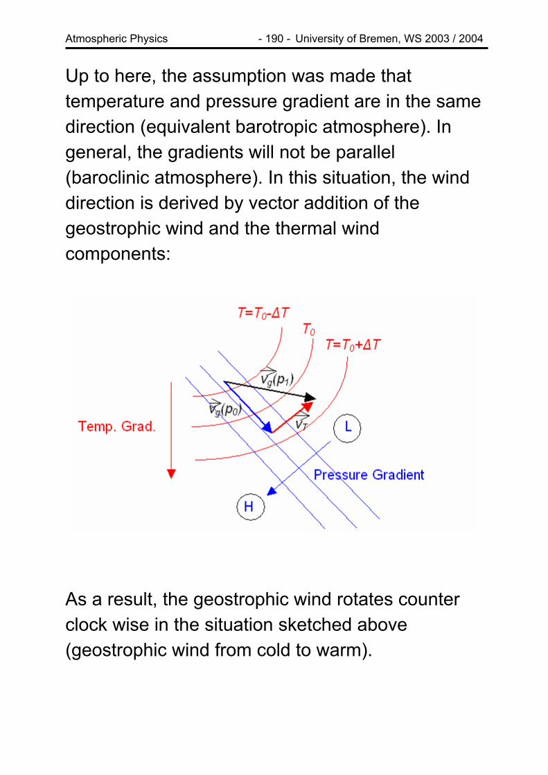
Atmospheric Physics - 190 - University of Bremen, WS 2003 / 2004
Up to here, the assumption was made that temperature and pressure gradient are in the same direction (equivalent barotropic atmosphere). In general, the gradients will not be parallel (baroclinic atmosphere). In this situation, the wind direction is derived by vector addition of the geostrophic wind and the thermal wind components:
As a result, the geostrophic wind rotates counter clock wise in the situation sketched above (geostrophic wind from cold to warm).
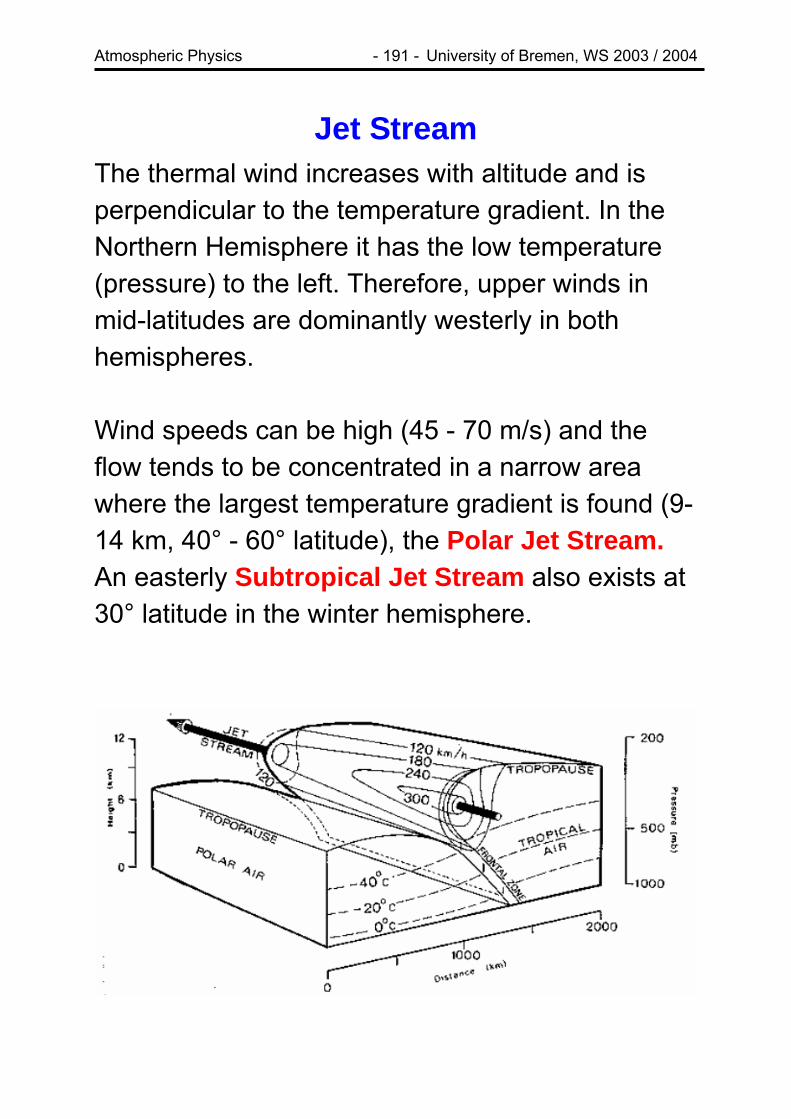
Atmospheric Physics - 191 - University of Bremen, WS 2003 / 2004
Jet Stream The thermal wind increases with altitude and is perpendicular to the temperature gradient. In the Northern Hemisphere it has the low temperature (pressure) to the left. Therefore, upper winds in mid-latitudes are dominantly westerly in both hemispheres. Wind speeds can be high (45 - 70 m/s) and the flow tends to be concentrated in a narrow area where the largest temperature gradient is found (9-14 km, 40° - 60° latitude), the Polar Jet Stream. An easterly Subtropical Jet Stream also exists at 30° latitude in the winter hemisphere.

Atmospheric Physics - 192 - University of Bremen, WS 2003 / 2004
The jet stream is close to the tropopause, and separates warm from cold regions. Depending on surface temperatures, it varies strongly from day to day. It is important for weather, transport and aviation.
Monday, January 12, 2004

Atmospheric Physics - 193 - University of Bremen, WS 2003 / 2004
Gradient Wind Observations show, that near low pressure the wind speed is up to 50% smaller than expected for a geostrophic wind (sub-geostrophic). This can be explained by the centrifugal force
Tcc R
vF2
ρ=
Fcc = centrifugal force v = wind speed
RT = local radius for the curvature of the isobars which near the low pressure system acts in the same direction as the Coriolis force but near the high pressure system has opposite direction:
Through Ridge
Atmospheric Physics - 194 - University of Bremen, WS 2003 / 2004
Therefore, wind speed near low pressure are lower and the curvature is smaller than near high pressure. At low latitudes where the Coriolis force becomes very small we have the so-called Cyclostrophic Balance where we find
0with2
≈≈= cpT
cc FFRvF ρ
.
A good example for this case is a hurricane Example: We assume a strong hurricane at 20o north. At 50 km from the centre we have a pressure gradient of 50 hPa per 100 km and assume ρ = 1.25 kg m-3:
m/s45m/s105010
105025.11
1
35
2
2
≈→⋅⋅
=
∂∂
=
∂∂
≈
=
vv
Rxpv
xp
Rv
FF
T
T
pcc
ρ
ρ

Atmospheric Physics - 195 - University of Bremen, WS 2003 / 2004
Continuity Equation In the atmosphere, the mass of an air parcel will be conserved. If it is compressed in the horizontal direction, it will expand in the vertical direction. As the troposphere is vertically limited by the surface and the tropopause, a convergence close to the ground will lead to ascent and then divergence at a higher altitude:
This is a crucial mechanism linking high and low pressure systems to vertical transport and therefore the formation of clouds and precipitation.
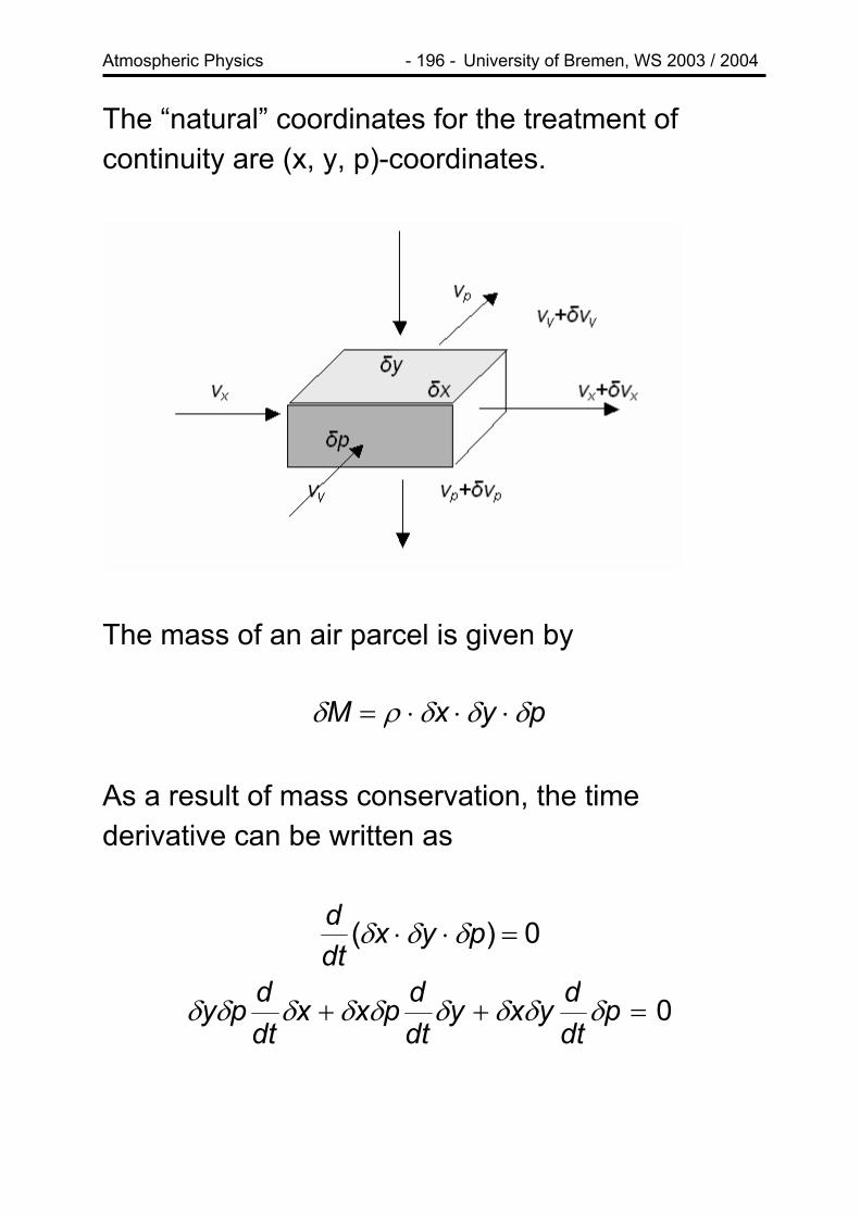
Atmospheric Physics - 196 - University of Bremen, WS 2003 / 2004
The “natural” coordinates for the treatment of continuity are (x, y, p)-coordinates.
The mass of an air parcel is given by
pyxM δδδρδ ⋅⋅⋅=
As a result of mass conservation, the time derivative can be written as
0)( =⋅⋅ pyxdtd δδδ
0=++ pdtdyxy
dtdpxx
dtdpy δδδδδδδδδ
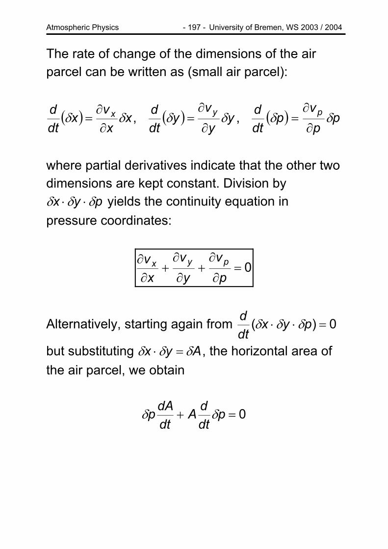
Atmospheric Physics - 197 - University of Bremen, WS 2003 / 2004
The rate of change of the dimensions of the air parcel can be written as (small air parcel):
( ) xx
vxdtd x δδ
∂∂
= , ( ) yyv
ydtd y δδ
∂
∂= , ( ) p
pv
pdtd p δδ
∂
∂=
where partial derivatives indicate that the other two dimensions are kept constant. Division by
pyx δδδ ⋅⋅ yields the continuity equation in pressure coordinates:
0=∂
∂+
∂
∂+
∂∂
pv
yv
xv pyx
Alternatively, starting again from 0)( =⋅⋅ pyxdtd δδδ
but substituting Ayx δδδ =⋅ , the horizontal area of the air parcel, we obtain
0=+ pdtdA
dtdAp δδ
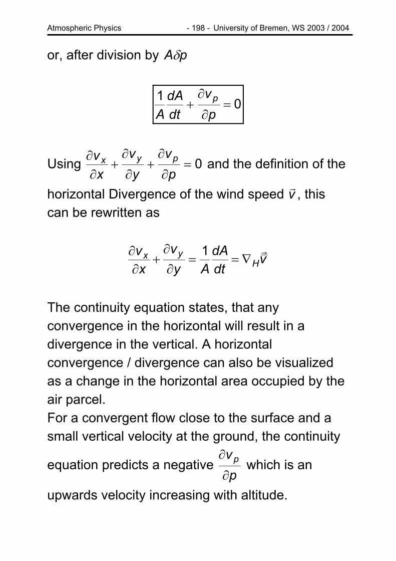
Atmospheric Physics - 198 - University of Bremen, WS 2003 / 2004
or, after division by pAδ
01=
∂
∂+
pv
dtdA
Ap
Using 0=∂
∂+
∂
∂+
∂∂
pv
yv
xv pyx and the definition of the
horizontal Divergence of the wind speed v , this can be rewritten as
r
vdtdA
Ayv
xv
Hyx r
∇==∂∂
+∂∂ 1
The continuity equation states, that any convergence in the horizontal will result in a divergence in the vertical. A horizontal convergence / divergence can also be visualized as a change in the horizontal area occupied by the air parcel. For a convergent flow close to the surface and a small vertical velocity at the ground, the continuity
equation predicts a negative p
vp
∂
∂ which is an
upwards velocity increasing with altitude.

Atmospheric Physics - 199 - University of Bremen, WS 2003 / 2004
Example:
A large cumulonimbus is observed from a geostationary satellite. From the increase in anvil area (20% in 10 minutes) the vertical velocity at the base of the anvil can be estimated:
)( vdp
dvH
p r∇−=
Integration from p1 to p:
∫ ∇−=p
pH dpvpvpv
1
)()()( 1r
Using the relation between divergence and area change
141033.3600
20.01 −−⋅≈≈=∇ sdtdA
AvHr
and assuming that v(100hPa) = 0 m/s, we obtain
hPa/s 2001033.30)300hPa( 4 ⋅⋅−= −pv

Atmospheric Physics - 200 - University of Bremen, WS 2003 / 2004
Assuming a scale height H = 7km, we can finally convert to a vertical velocity vz averaged over the anvil:
m/s5.1)hPa300()hPa300( ≈=pHvv pz
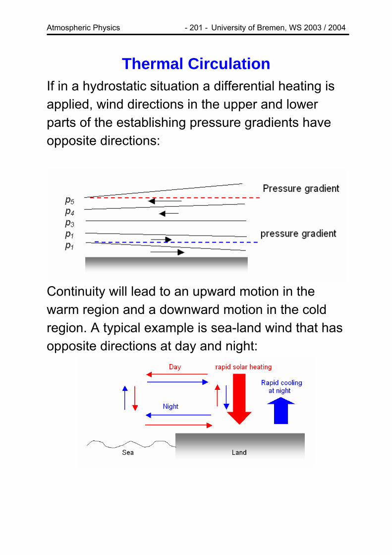
Atmospheric Physics - 201 - University of Bremen, WS 2003 / 2004
Thermal Circulation If in a hydrostatic situation a differential heating is applied, wind directions in the upper and lower parts of the establishing pressure gradients have opposite directions:
Continuity will lead to an upward motion in the warm region and a downward motion in the cold region. A typical example is sea-land wind that has opposite directions at day and night:
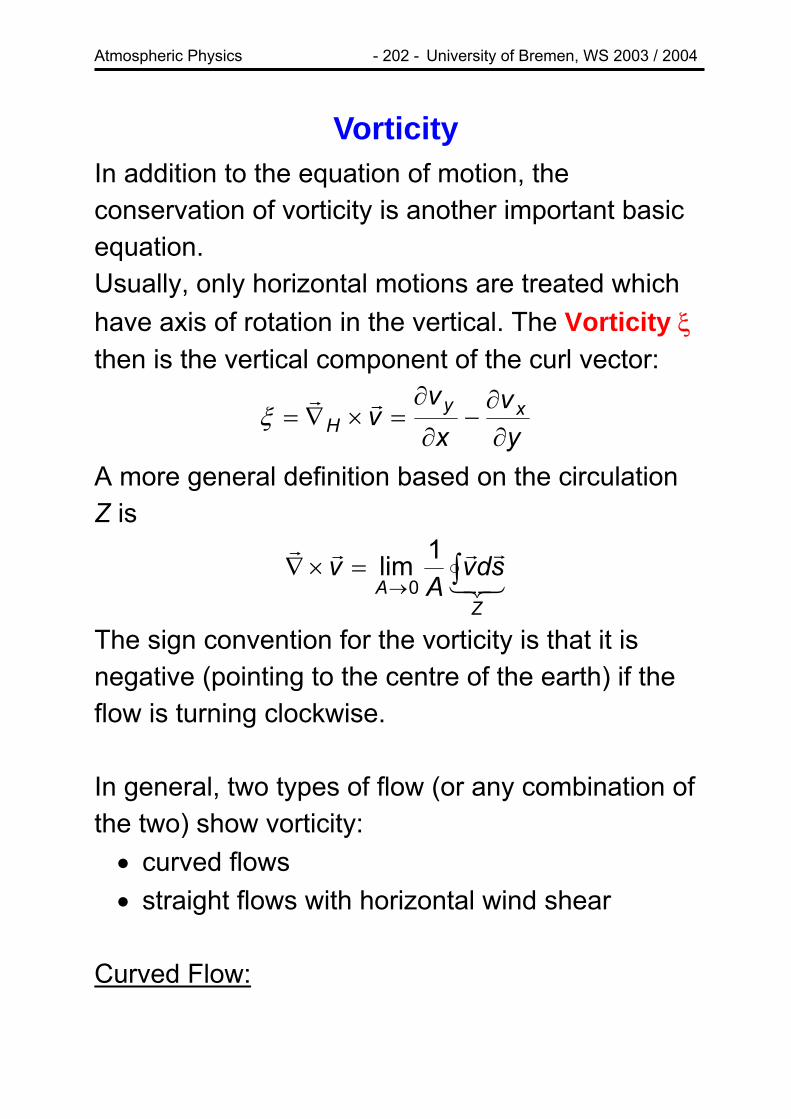
Atmospheric Physics - 202 - University of Bremen, WS 2003 / 2004
Vorticity In addition to the equation of motion, the conservation of vorticity is another important basic equation. Usually, only horizontal motions are treated which have axis of rotation in the vertical. The Vorticity ξ then is the vertical component of the curl vector:
yv
xv
v xyH ∂
∂−
∂
∂=×∇=
rrξ
A more general definition based on the circulation Z is
321
rrrr
ZA
sdvA
v ∫→
=×∇1lim
0
The sign convention for the vorticity is that it is negative (pointing to the centre of the earth) if the flow is turning clockwise. In general, two types of flow (or any combination of the two) show vorticity: • curved flows • straight flows with horizontal wind shear
Curved Flow:

Atmospheric Physics - 203 - University of Bremen, WS 2003 / 2004
The simplest situation for a curved flow is the rotation, for which the speed is simply
rv ω= The circulation Z can thus be computed as
222 rrvvdsZ πωπ === ∫
Division by the area yields
ωπ
ξ 22 ==rZ
which is just two times the angular velocity. For a general curved flow, one can derive that
rv
rrv
∂∂
+=)(ξ

Atmospheric Physics - 204 - University of Bremen, WS 2003 / 2004
Shear Flow: The basic idea of why a shear flow has a vorticity becomes clear when imagining what the motion of a stick would be in such a flow:
The value of this kind of vorticity follows immediately from the definition in cartesian coordinates.

Atmospheric Physics - 205 - University of Bremen, WS 2003 / 2004
On the rotating Earth, the absolute vorticity η is the sum of the vorticity of the parcel moving in the atmosphere and the vorticity of the rotating Earth:
f+= ξη where ϕsin2Ω=f is the Coriolis parameter and the units are s-1. On the Southern Hemisphere, the sign of f has to be set to minus f−= ξη . If there are no external forces, the absolute vorticity is conserved, and a continuity equation can be formulated:
0)( =+∂∂ vdiv
t Hr
ηη
It should be noted that the vorticity equation is not independent of the equation of motion but can be derived from it by taking the Rotation of both sides and performing some algebra.

Atmospheric Physics - 206 - University of Bremen, WS 2003 / 2004
Potential Vorticity A quantity related to the absolute vorticity is the potential vorticity, which combines the conservation of vorticity and mass. The most frequently used definition is that of Ertel’s Potential Vorticity (PV)
dzdZEΘ
=ρη
Θ = potential temperature ρ = density
or equivalently
⎟⎠
⎞⎜⎝
⎛ Θ−=
dpdgZE η
The units of PV are [K m2 kg-1 s-1], sometimes also abbreviated as PVU. As long as only adiabatic processes take place, Ertel’s PV is a conserved quantity. It therefore can be used as a tracer of air mass origin in the atmosphere.
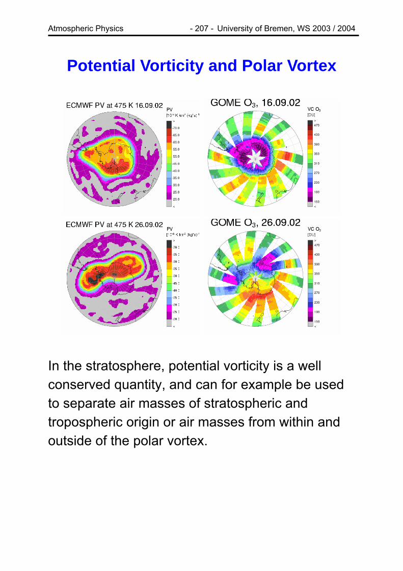
Atmospheric Physics - 207 - University of Bremen, WS 2003 / 2004
Potential Vorticity and Polar Vortex
In the stratosphere, potential vorticity is a well conserved quantity, and can for example be used to separate air masses of stratospheric and tropospheric origin or air masses from within and outside of the polar vortex.
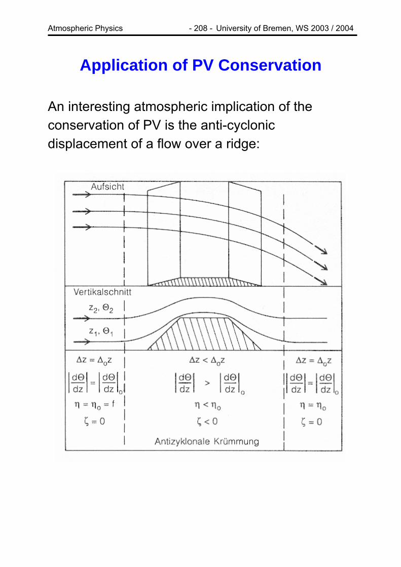
Atmospheric Physics - 208 - University of Bremen, WS 2003 / 2004
Application of PV Conservation An interesting atmospheric implication of the conservation of PV is the anti-cyclonic displacement of a flow over a ridge:

Atmospheric Physics - 209 - University of Bremen, WS 2003 / 2004
When a parallel flow has to overcome a ridge (mountains, a continent), the distance between levels of potential temperature will be reduced and
thereby dzdΘ increases. Thus the vorticity η has to
decrease. Assuming an initial flow with η = f and disregarding changes in f, the flow will get an anti-cyclonic component after the ridge. Under certain conditions, this can give rise to a wave (see discussion of Lee-waves), for example in the Rossby waves.
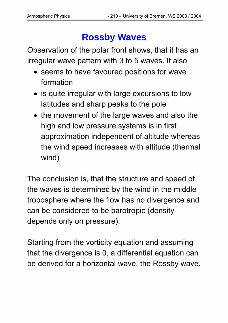
Atmospheric Physics - 210 - University of Bremen, WS 2003 / 2004
Rossby Waves Observation of the polar front shows, that it has an irregular wave pattern with 3 to 5 waves. It also • seems to have favoured positions for wave
formation • is quite irregular with large excursions to low
latitudes and sharp peaks to the pole • the movement of the large waves and also the
high and low pressure systems is in first approximation independent of altitude whereas the wind speed increases with altitude (thermal wind)
The conclusion is, that the structure and speed of the waves is determined by the wind in the middle troposphere where the flow has no divergence and can be considered to be barotropic (density depends only on pressure). Starting from the vorticity equation and assuming that the divergence is 0, a differential equation can be derived for a horizontal wave, the Rossby wave.
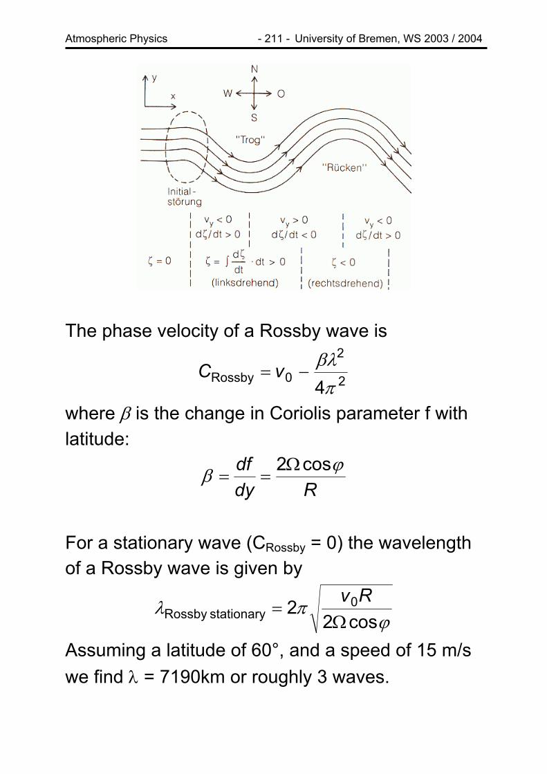
Atmospheric Physics - 211 - University of Bremen, WS 2003 / 2004
The phase velocity of a Rossby wave is
2
2
0Rossby 4πβλ
−= vC
where β is the change in Coriolis parameter f with latitude:
Rdydf ϕβ cos2Ω
==
For a stationary wave (CRossby = 0) the wavelength of a Rossby wave is given by
ϕπλ
cos22 0
stationary Rossby Ω=
Rv
Assuming a latitude of 60°, and a speed of 15 m/s we find λ = 7190km or roughly 3 waves.

Atmospheric Physics - 212 - University of Bremen, WS 2003 / 2004
Comments on Rossby waves: • the phase velocity is always smaller than the
flow velocity • larger wavelengths correspond to slower wave
speed. In the atmosphere, different wave speeds overlay and therefore smaller waves move through the slower larger waves.
• a very large wave could even proceed in the opposite direction
• Rossby waves are stable, and can not explain the development of cyclones or fronts
Rossby waves can also propagate in three dimensions and link tropospheric and stratospheric dynamics. An important example are major warmings in the stratosphere that can break up the winter polar vortex by dissipating energy in the upper stratosphere and reversing the general flow direction from cyclonic to anti-cyclonic.

Atmospheric Physics - 213 - University of Bremen, WS 2003 / 2004
Frontal Systems The interfaces between cold and warm air masses are called fronts. They are regions of strong thermal winds that often extend over hundreds of kilometres.
Cold front: cold air advances and pushes warm air up Warm front: warm air advances and glides on cold air Stationary front: a front that is not moving Occluded front: warm air is lifted up by cold air from a fast cold front that is overtaking a warm front
At the polar front, cyclones are generated from instabilities in Rosby waves. They are accompanied by cloud formation, precipitation and strong winds. They also create a net flow of energy from lower to higher latitudes.
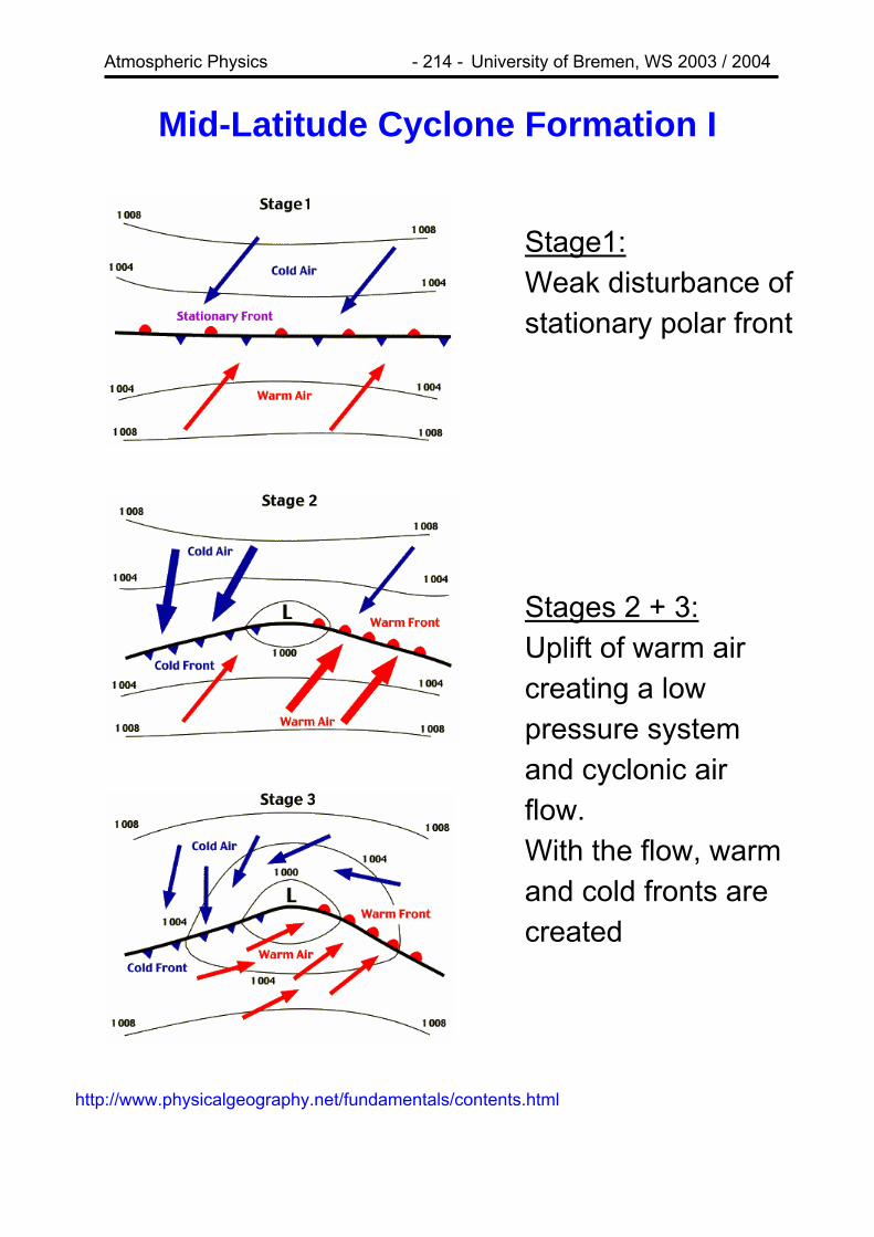
Atmospheric Physics - 214 - University of Bremen, WS 2003 / 2004
Mid-Latitude Cyclone Formation I
Stage1: Weak disturbance of stationary polar front Stages 2 + 3: Uplift of warm air creating a low pressure system and cyclonic air flow. With the flow, warm and cold fronts are created
http://www.physicalgeography.net/fundamentals/contents.html

Atmospheric Physics - 215 - University of Bremen, WS 2003 / 2004
Mid-Latitude Cyclone Formation II
Stages 4 + 5: Pressure drops and the storm intensifies, the trough gets sharper as wind speeds increase. Stage 6: The cold front overtakes the warm front lifting the warm air in the upper atmosphere

Atmospheric Physics - 216 - University of Bremen, WS 2003 / 2004
Mid-Latitude Cyclone Formation III
Stage 7: The uplifting leads to an occluded front Stages 8 + 9: The occlusion dissolves, winds subside and the stationary front is reformed. The lifetime of such a cyclone is 3-10 days.
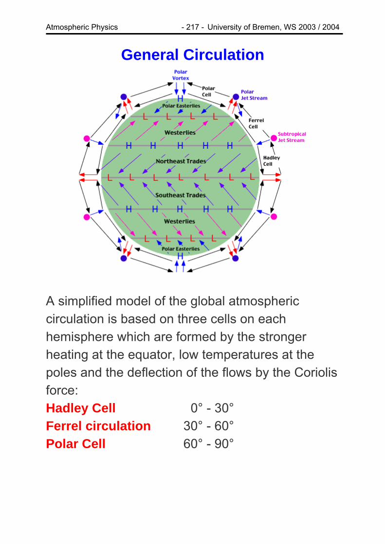
Atmospheric Physics - 217 - University of Bremen, WS 2003 / 2004
General Circulation
A simplified model of the global atmospheric circulation is based on three cells on each hemisphere which are formed by the stronger heating at the equator, low temperatures at the poles and the deflection of the flows by the Coriolis force: Hadley Cell 0° - 30° Ferrel circulation 30° - 60° Polar Cell 60° - 90°

Atmospheric Physics - 218 - University of Bremen, WS 2003 / 2004
Hadley cell:
• thermal wind • convection / convergence leads to rising air
over the tropics (ITCZ) • movement to higher latitudes • deflection by Coriolis force • formation of subtropical jet stream (STJ) • accumulation through transport leads to
sinking air at 30° • formation of subtropical high • most air moves back to equator close to the
surface to close the cell • again: deflection by Coriolis force => trade
winds

Atmospheric Physics - 219 - University of Bremen, WS 2003 / 2004
Eastward velocities in the upper part of the Hadley cell can be quite large as a simple estimate from angular momentum conservation shows:
[ ] constRvRL
constJL
=+Ω=
=+Ω=
)cos/()cos(
)(2 ϕϕ
ω
L = angular momentum per mass J = moment of inertia
ω = angular velocity relative to the earth ϕ = latitude, R = earth radius
Starting with a flow at the equator (ϕ = 0) with no zonal velocity component (v = 0) we obtain
[ ])cos/(cos222 ϕϕ RvRR +Ω=Ω or
ϕϕϕ
ϕ tansincos
)cos1( 2Ω=
−Ω= RRv
With RΩ = 40000 km/day ≈ 450 m/s the eastward velocity at 30° is about v = 130 m/s. Measured wind speeds are lower on average (20 - 50 m/s depending on season) but can reach 100 m/s in the subtropical jets.

Atmospheric Physics - 220 - University of Bremen, WS 2003 / 2004
Ferrel circulation: • only exists in averaged winds • high pressure systems tend to form in the
subtropics while low pressure systems tend be located at the polar front. In low pressure systems air ascends while it descends in high pressure systems, horizontal winds balance => on average, a cell is formed
• the Ferrel circulation is thermally indirect
Polar Cell • thermally direct • driven by cold surface winds from the poles to
mid-latitudes • wind deflection by Coriolis force

Atmospheric Physics - 221 - University of Bremen, WS 2003 / 2004
Example: January 20, 2004
• cloud band from South America over Southern Africa to the Pacific: convection in the ITCZ
• cloud band north of Antarctica • cloud system from North America to Europe • no clouds over central Asia • no clouds over North Africa • few clouds over southern US / Mexico

Atmospheric Physics - 222 - University of Bremen, WS 2003 / 2004
Sea-Level Pressure and Surface Winds
JUL
JAN
http://www.physicalgeography.net/fundamentals/7p.html

Atmospheric Physics - 223 - University of Bremen, WS 2003 / 2004
The real situation differs from the simple model because • land and ocean have very different heating
rates and therefore temperature differences establish that change with season
• surface height intensifies pressure systems, in particular high pressure systems
• the tilt of the earth’s rotation axis leads to a latitudinal movement of the area of largest and lowest heating
As a result, the intertropical convergence zone • moves with season • extends further polewards over continents
The subtropical high pressure zone is divided into individual high pressure centres intensify where (relatively) cold air masses form, which is over the sea in summer and over land in winter. The subpolar lows form a continuous zone in the Southern Hemisphere but not in the North. They are a result of the large latitudinal temperature differences.

Atmospheric Physics - 224 - University of Bremen, WS 2003 / 2004
Differences between the Hemispheres The atmospheric situation is not symmetric with respect to the equator, mainly as a result of the unequal distribution of land masses: • meridional energy exchange is larger in the NH
as friction over the continents and local disturbances of the flow increase the non-geostrophic wind component
• the radiation budget of Antarctica is more negative than that of the Arctic
• zonal winds are less disturbed by topography in the SH
As a result, meridional temperature and pressure differences are much larger in the SH, which leads to higher wind speeds and leads to important differences in the stratosphere (ozone hole). Another consequence is, that the ITCZ is at 5°N on average, and has very different shapes in summer and winter.
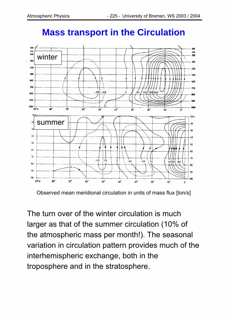
Atmospheric Physics - 225 - University of Bremen, WS 2003 / 2004
Mass transport in the Circulation
Observed mean meridional circulation in units of mass flux [ton/s]
winter
summer
The turn over of the winter circulation is much larger as that of the summer circulation (10% of the atmospheric mass per month!). The seasonal variation in circulation pattern provides much of the interhemispheric exchange, both in the troposphere and in the stratosphere.

Atmospheric Physics - 226 - University of Bremen, WS 2003 / 2004
Monsoon The basic principle behind the monsoon is similar to that of the sea breeze: differential heating over land and sea.

Atmospheric Physics - 227 - University of Bremen, WS 2003 / 2004
In summer, air over the continents warms and ascends, and moist, colder air flows in from the ocean bringing heavy rain. The latent heat release and continuous solar insolation stabilise the circulation which can continue for months. The winter monsoon has the same origin but opposite direction as the tropical sea is warmer in winter and brings draught rather than rain. Monsoon patterns extend over East Africa, Arabia, India, and the Arabian Sea. Similar but weaker patterns can also be found in equatorial America. Summer monsoon over India is a result of the low pressure zone over the Asian highlands that move North with the sun, leading to monsoon patterns appearing first in Sri Lanka end of May and moving to the Himalayas by July. They lead to the highest rainfall values observed anywhere on earth.

Atmospheric Physics - 228 - University of Bremen, WS 2003 / 2004
Aside: Transport of Pollutants In the industrialized regions and in regions of biomass burning, large amounts of pollutants are emitted. Many secondary pollutants are the result of intense photochemistry (e.g. ozone). How far pollutants will be transported depends on their lifetime and on wind speeds. Wind speeds are much larger in the upper troposphere, and therefore long range transport is favoured where convection carries things upwards. The tropics are a very relevant area for large scale pollution because • interhemispheric exchange dominated by ITCZ
movement • transport from troposphere to stratosphere
mainly in the ITCZ • convective activity in tropical regions favours
long range transport of pollutants • large insolation in the tropics favours
photochemistry • population density and degree of
industrialisation is high and increasing
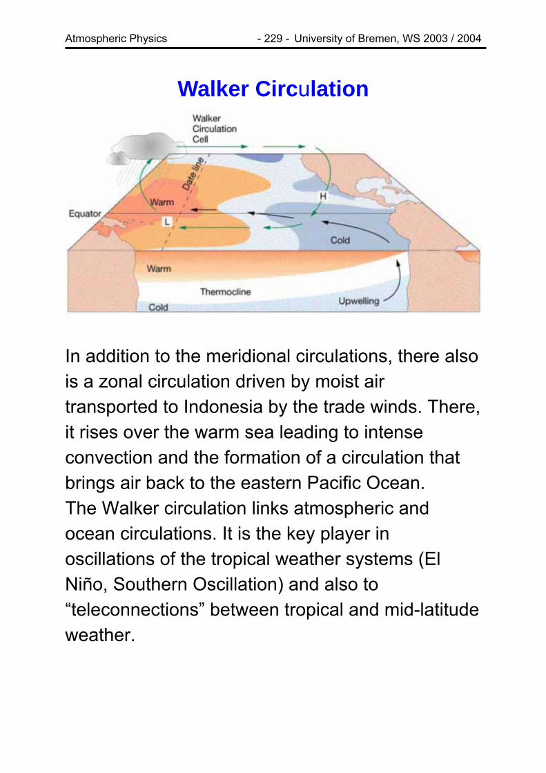
Atmospheric Physics - 229 - University of Bremen, WS 2003 / 2004
Walker Circulation
In addition to the meridional circulations, there also is a zonal circulation driven by moist air transported to Indonesia by the trade winds. There, it rises over the warm sea leading to intense convection and the formation of a circulation that brings air back to the eastern Pacific Ocean. The Walker circulation links atmospheric and ocean circulations. It is the key player in oscillations of the tropical weather systems (El Niño, Southern Oscillation) and also to “teleconnections” between tropical and mid-latitude weather.
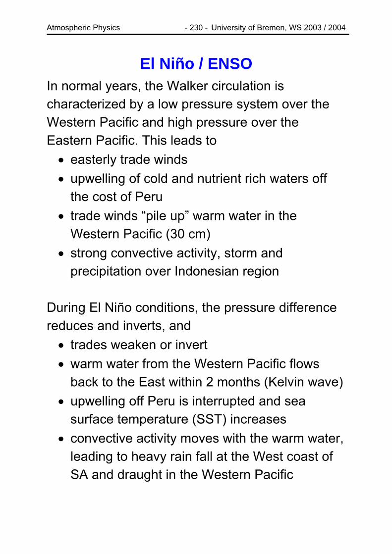
Atmospheric Physics - 230 - University of Bremen, WS 2003 / 2004
El Niño / ENSO In normal years, the Walker circulation is characterized by a low pressure system over the Western Pacific and high pressure over the Eastern Pacific. This leads to • easterly trade winds • upwelling of cold and nutrient rich waters off
the cost of Peru • trade winds “pile up” warm water in the
Western Pacific (30 cm) • strong convective activity, storm and
precipitation over Indonesian region During El Niño conditions, the pressure difference reduces and inverts, and • trades weaken or invert • warm water from the Western Pacific flows
back to the East within 2 months (Kelvin wave) • upwelling off Peru is interrupted and sea
surface temperature (SST) increases • convective activity moves with the warm water,
leading to heavy rain fall at the West coast of SA and draught in the Western Pacific
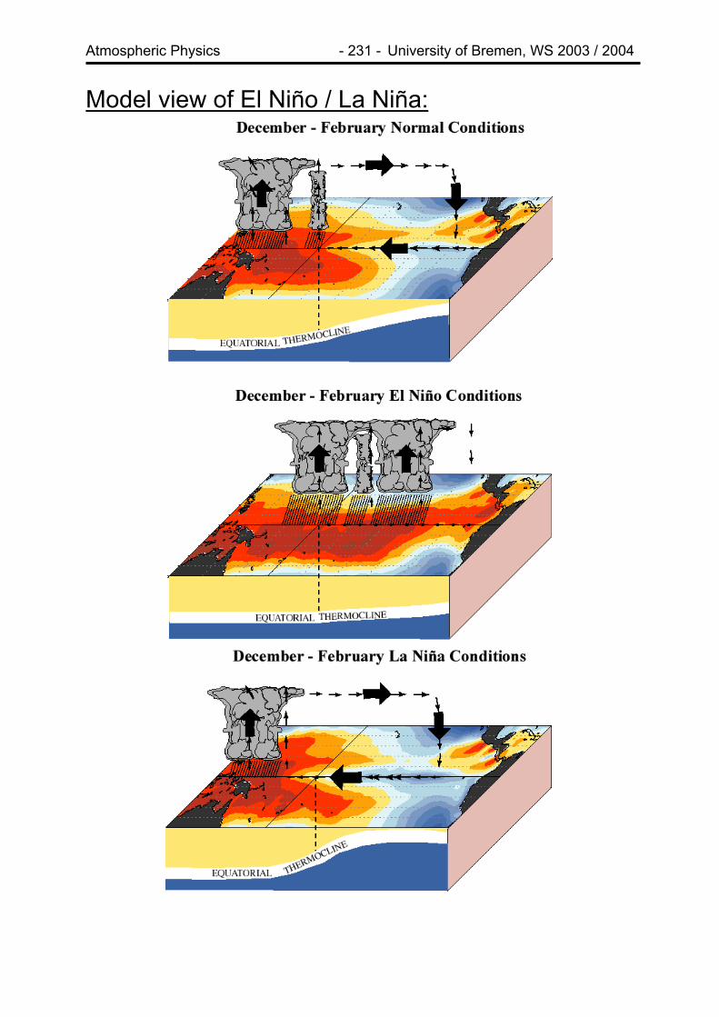
Atmospheric Physics - 231 - University of Bremen, WS 2003 / 2004
Model view of El Niño / La Niña:

Atmospheric Physics - 232 - University of Bremen, WS 2003 / 2004
http://www.cpc.ncep.noaa.gov/products/analysis_monitoring/ensocycle/ensocycle.html
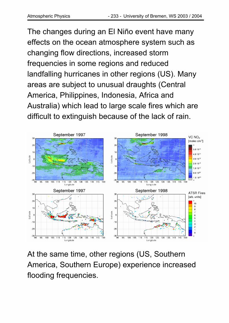
Atmospheric Physics - 233 - University of Bremen, WS 2003 / 2004
The changes during an El Niño event have many effects on the ocean atmosphere system such as changing flow directions, increased storm frequencies in some regions and reduced landfalling hurricanes in other regions (US). Many areas are subject to unusual draughts (Central America, Philippines, Indonesia, Africa and Australia) which lead to large scale fires which are difficult to extinguish because of the lack of rain.
At the same time, other regions (US, Southern America, Southern Europe) experience increased flooding frequencies.
Atmospheric Physics - 234 - University of Bremen, WS 2003 / 2004
La Niña, Southern Oscillation At the end of an El Niño event, the high pressure system over the Eastern Pacific re-establishes, and the region of convection moves back to the west. During this period, the normal situation is somewhat exaggerated, again leading to extreme weather conditions, although with less impact on human activities.
El Niño and La Niña events can be measured by the ocean temperature differences or the Southern Oscillation Index (SOI), that gives the difference of surface pressure between Tahiti and Darwin.

Atmospheric Physics - 235 - University of Bremen, WS 2003 / 2004
Stratospheric Dynamics Stratospheric dynamics is driven by similar forces as the tropospheric dynamics: • temperature gradients, mainly from the tropics
to the poles • Coriolis force • continuity equation (mass conservation)
The main differences between stratosphere and troposphere are • the stratosphere has a stable temperature
profile • air density is low • stratospheric air is very dry (dry freezing of air
in the tropopause) => no latent heat release • air tends to remain on isentropic surfaces for
many days; vertical motions are very small • diabatic processes (mainly heating and cooling
through radiation) are relevant • the tropics are not always warmer than the
poles! In the lower and middle stratosphere, ozone can be used as a tracer for air masses.
see: http://www.ccpo.odu.edu/SEES/ozone/class/Chap_6/

Atmospheric Physics - 236 - University of Bremen, WS 2003 / 2004
The stratosphere can be divided in several parts:
tropics: region 20°S - 20°N, upward transport of
air, ozone formation surf zone: middle latitudes of the stratosphere -
“turbulent” mixing of different air masses, more pronounced in the NH
polar vortex: strong westerlies form in the region of the polar night terminator forming the polar night jet which separates polar from mid-latitude air masses
lowermost stratosphere: region of mixture between tropospheric and stratospheric air, roughly between tropopause and 380K potential temperature

Atmospheric Physics - 237 - University of Bremen, WS 2003 / 2004
The change in temperature gradient between winter and summer hemisphere implies that winds are westerly in winter (Polar Vortex) but easterly in summer. The turn over is observed in spring at the final warming which is much later in the SH than in the NH. Note: the stratospheric polar night jet should not be confused with the tropospheric polar jet stream which is present throughout the year. In the polar vortex, air cools diabatically by radiation and therefore a net downward movement is observed in the vortex. Observations show, that stratospheric tempera-tures in the SH are much lower than in the NH and that the surf zone is less pronounced in the SH. Also, temperatures in the polar vortex are much higher than a simple model would predict from radiation balance. Thus, a mechanism for energy transport from the tropics to the pole must exist.

Atmospheric Physics - 238 - University of Bremen, WS 2003 / 2004
Brewer-Dobson Circulation
In the winter hemisphere, a circulation establishes that is driven by • large-scale ascent in the tropics (20-30 m/day) • descent in the polar vortex • a wave driven poleward and downward
pumping in the surf zone • stratosphere / troposphere exchange in the
lowermost stratosphere In the summer hemisphere, only a weak circulation exists.

Atmospheric Physics - 239 - University of Bremen, WS 2003 / 2004
Surf Zone In the surf zone, large scale planetary (Rossby) waves form, starting in the troposphere and propagating into the stratosphere:
Waves break in the upper stratosphere and deposit energy and easterly momentum there,
Atmospheric Physics - 240 - University of Bremen, WS 2003 / 2004
which decreases the speed of the westerly wintertime stratospheric jet stream. Decreasing speed means decreasing Coriolis force which induces a poleward component of the flow, similar to the effect of friction on geostrophic wind in the troposphere. Air RISES over the equator, drifts steadily POLEWARD (while meandering around the latitude circles) and SINKS at the poles.
If the Rossby wave is very strong or the circulation weakened, the temperature gradient can be inverted and the vortex breaks down. As a result of the smaller land - ocean contrast in the SH, planetary waves are much less frequent in the SH, and therefore transport is weaker, the vortex faster and colder and the time of vortex break up in spring much delayed compared to the NH. This is the prerequisite for the Ozone Hole observed in the southern hemisphere every winter / spring.

Atmospheric Physics - 241 - University of Bremen, WS 2003 / 2004
Stratospheric Transport by Waves Waves induced by tropospheric weather systems can trigger strong meridional transport as can be observed in stratospheric ozone measurements:
The polar vortex is distorted and shifted by a wave, and low latitude air moves north while polar air moves to the equator. If the extrusion is long enough, it will separate from the vortex and mix irreversible with the surroundings, constituting a net transport of air (shown here in the ozone field).

Atmospheric Physics - 242 - University of Bremen, WS 2003 / 2004
Stratospheric Ozone Stratospheric ozone columns are largely determined by transport. Their magnitude does not correlate well with illumination which is high over the tropics and low in winter at high latitudes. Also, a marked difference between the two hemispheres is observed:

Atmospheric Physics - 243 - University of Bremen, WS 2003 / 2004
The observed stratospheric ozone distribution (without ozone loss chemistry) can be explained by the Brewer-Dobson circulation: • formation of ozone in the ascending air in the
tropics • poleward transport • downward transport and accumulation at mid-
and high-latitudes • largest columns in NH winter polar vortex (less
wave activity and thus transport in the SH).
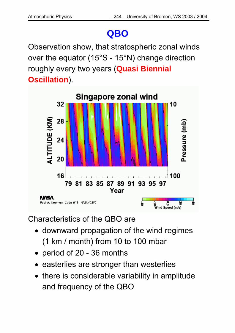
Atmospheric Physics - 244 - University of Bremen, WS 2003 / 2004
QBO Observation show, that stratospheric zonal winds over the equator (15°S - 15°N) change direction roughly every two years (Quasi Biennial Oscillation).
Characteristics of the QBO are • downward propagation of the wind regimes
(1 km / month) from 10 to 100 mbar • period of 20 - 36 months • easterlies are stronger than westerlies • there is considerable variability in amplitude
and frequency of the QBO

Atmospheric Physics - 245 - University of Bremen, WS 2003 / 2004
The theory of the QBO is complicated and not fully developed (many atmospheric models do not create a QBO on their own). It is now thought that equatorially trapped Kelvin waves provide the westerly momentum and Rossby-gravity waves provide easterly momentum to produce the QBO oscillation. The QBO is linked to many atmospheric processes such as • ozone columns (changes in transport) • hurricane frequencies in the Atlantic (lower for
easterly QBO) • ENSO and the monsoon • major winter stratospheric warmings which
preferentially occur during the easterly phase of the QBO
Atmospheric Physics - 246 - University of Bremen, WS 2003 / 2004
Stratosphere-Troposphere Exchange Exchange between the stratosphere and troposphere is relevant for anthropogenic influences on the stratospheric ozone layer, climate changes and the link between tropospheric and stratospheric dynamics. Two different views can be taken on the STE: 1) the global view, where the relevant exchange is through the 380 K isentrope and exchange is governed by the large scale circulation in the stratosphere 2) the local view, where exchange through the tropopause is treated, which is possible through • convective overshooting in the tropics • horizontal transport through tropopause folds • cut-off low pressure systems that become
separated from the main flow of the upper tropospheric jet stream, usually associated with blocking patterns and can travel upwards through the tropopause