lecture notes discrete optimization - universiteit …kernw/lectures/do/do_script.pdflecture notes...
TRANSCRIPT

Document last modified: January 10, 2012
Lecture Notes of the Master Course:
Discrete OptimizationUtrecht UniversityAcademic Year 2011/2012
Course website:http://www.cwi.nl/˜schaefer/courses/lnmb-do11
Prof. dr. Guido Schafer
Center for Mathematics and Computer Science (CWI)Algorithms, Combinatorics and Optimization GroupScience Park 123, 1098 XG Amsterdam, The Netherlands
VU University AmsterdamDepartment of Econometrics and Operations ResearchDe Boelelaan 1105, 1081 HV Amsterdam, The Netherlands
Website:http://www.cwi.nl/˜schaeferEmail: [email protected]
Document last modified:January 10, 2012
Disclaimer: These notes contain (most of) the material of the lectures ofthe course “Dis-crete Optimization”, given at Utrecht University in the academic year 2011/2012. Thecourse is organized by theDutch Network on the Mathematics of Operations Research(LNMB) and is part of theDutch Master’s Degree Programme in Mathematics (Master-math). Note that the lecture notes have undergone some rough proof-reading only. Pleasefeel free to report any typos, mistakes, inconsistencies, etc. that you observe by sendingme an email ([email protected]).

Note that these Lecture Notes have been last modified on January 10, 2012. I guess mostof you will have printed the Lecture Notes of December 6, 2011(see “document lastmodified” date on your printout). I therefore keep track of the changes that I made sincethen below. I also mark these changes as “[major]” or “[minor]”, depending on theirimportance.
Changes made with respect to Lecture Notes of December 6, 2011:
• [major ] Introducing the notion of a pseudoflow on page 42: corrected“it needto satisfy the flow balance constraints” to “it neednot satisfy the flow balanceconstraints”.
Changes made with respect to Lecture Notes of December 20, 2011: (Thanks to RutgerKerkkamp for pointing these out.)
• [minor] Symbol for symmetric difference on page 4 is now the same as the oneused in Chapter 7 (“”).• [minor] Strictly speaking we would have to add a constraintx j ≤ 1 for every j ∈1, . . . ,n to the LP relaxation (2) of the integer linear program (1) on page 5.However, these constraints are often (but not always) redundant because of theminimization objective. Note that the discussion that follows refers to the LPrelaxation as stated in (2) (see also remark after statementof LP (2)).• [minor] Corrected “multiplies” to “multipliers” in last paragraph on page 5.• [minor] Lower part of Figure 2 on page 2: changed edgee from solid to dotted
line.• [minor] At various places in Chapter 3, Condition (M1) of theindependent set sys-
tem has not been mentioned explicitly (Example 3.1, Examples 3.3–3.5, Theorem3.1). Mentioned now.• [minor] Corrected “many application” to “many applications” in first paragraph
on page 27.• [minor] Corrected “δ (v)” and “δ (u)” to “ δ (s,v)” and “δ (s,u)” in last paragraph
of the proof of Lemma 5.5. on page 34 (3 occurrences).• [minor] Algorithms 7 and 8 should mention that the capacity function is non-
negative.• [major ] There was a mistake in the objective function of the dual linear program
(6) on page 46: The sign in front of the second summation must be negative.• [minor] Algorithms 9, 10 and 11 should mention that the capacity function is non-
negative.• [minor] Proof of Theorem 7.3 on page 56: corrected “O(mα(n,m))” to
“O(mα(n, mn ))”.
• [minor] Caption of the illustration on page 71 has been put onthe same page.• [minor] Typo in the second last sentence of the proof of Theorem 6.7 on page 47:
“cπ(u,v)< 0” corrected to “cπ(u,v)≤ 0”.• [minor] Statement of Theorem 10.8 on page 90 has been corrected (FPTAS instead
of 2-approximation).

Changes made with respect to Lecture Notes of January 5, 2012: (Thanks to Tara vanZalen and Arjan Dijkstra for pointing these out.)
• [minor] Example 3.2 on page 21 (uniform matroids): corrected “I = I ⊆S | |S|≤k” to “ I = I ⊆ S | |I | ≤ k”• [minor] Statement of Lemma 5.4 on page 32: corrected “The flowof any flow” to
“The flow value of any flow”.• [minor] There was a minus sign missing in the equation (7) on page 43.• [minor] Second paragraph of Section 8.3 on page 60: Corrected “hyperplance” to
“hyperplane”.• [minor] Removed sentence “We state the following proposition without proof”
before statement of Lemma 8.4 on page 62.• Corrected “Note hatb is integral” to “Note thatb is integral” in the proof of The-
orem 8.7 on page 63.
Please feel free to report any mistakes, inconsistencies, etc. that you encounter.
Guido
ii
Contents
1 Preliminaries 1
1.1 Optimization Problems. . . . . . . . . . . . . . . . . . . . . . . . . . . 1
1.2 Algorithms and Efficiency . . . . . . . . . . . . . . . . . . . . . . . . . 2
1.3 Growth of Functions . . . . . . . . . . . . . . . . . . . . . . . . . . . . 3
1.4 Graphs. . . . . . . . . . . . . . . . . . . . . . . . . . . . . . . . . . . . 3
1.5 Sets, etc.. . . . . . . . . . . . . . . . . . . . . . . . . . . . . . . . . . . 4
1.6 Basics of Linear Programming Theory. . . . . . . . . . . . . . . . . . . 5
2 Minimum Spanning Trees 7
2.1 Introduction. . . . . . . . . . . . . . . . . . . . . . . . . . . . . . . . . 7
2.2 Coloring Procedure. . . . . . . . . . . . . . . . . . . . . . . . . . . . . 7
2.3 Kruskal’s Algorithm . . . . . . . . . . . . . . . . . . . . . . . . . . . . 10
2.4 Prim’s Algorithm . . . . . . . . . . . . . . . . . . . . . . . . . . . . . . 12
3 Matroids 14
3.1 Introduction. . . . . . . . . . . . . . . . . . . . . . . . . . . . . . . . . 14
3.2 Matroids. . . . . . . . . . . . . . . . . . . . . . . . . . . . . . . . . . . 15
3.3 Greedy Algorithm for Matroids. . . . . . . . . . . . . . . . . . . . . . . 16
4 Shortest Paths 18
4.1 Introduction. . . . . . . . . . . . . . . . . . . . . . . . . . . . . . . . . 18
4.2 Single Source Shortest Path Problem. . . . . . . . . . . . . . . . . . . . 18
4.2.1 Basic properties of shortest paths. . . . . . . . . . . . . . . . . 19
4.2.2 Arbitrary cost functions . . . . . . . . . . . . . . . . . . . . . . 21
4.2.3 Nonnegative cost functions. . . . . . . . . . . . . . . . . . . . . 22
4.3 All-pairs Shortest-path Problem. . . . . . . . . . . . . . . . . . . . . . 23
5 Maximum Flows 27
iii

5.1 Introduction. . . . . . . . . . . . . . . . . . . . . . . . . . . . . . . . . 27
5.2 Residual Graph and Augmenting Paths. . . . . . . . . . . . . . . . . . . 28
5.3 Ford-Fulkerson Algorithm. . . . . . . . . . . . . . . . . . . . . . . . . 30
5.4 Max-Flow Min-Cut Theorem. . . . . . . . . . . . . . . . . . . . . . . . 31
5.5 Edmonds-Karp Algorithm . . . . . . . . . . . . . . . . . . . . . . . . . 33
6 Minimum Cost Flows 36
6.1 Introduction. . . . . . . . . . . . . . . . . . . . . . . . . . . . . . . . . 36
6.2 Flow Decomposition and Residual Graph. . . . . . . . . . . . . . . . . 37
6.3 Cycle Canceling Algorithm. . . . . . . . . . . . . . . . . . . . . . . . . 40
6.4 Successive Shortest Path Algorithm. . . . . . . . . . . . . . . . . . . . 42
6.5 Primal-Dual Algorithm. . . . . . . . . . . . . . . . . . . . . . . . . . . 46
7 Matchings 51
7.1 Introduction. . . . . . . . . . . . . . . . . . . . . . . . . . . . . . . . . 51
7.2 Augmenting Paths. . . . . . . . . . . . . . . . . . . . . . . . . . . . . . 51
7.3 Bipartite Graphs. . . . . . . . . . . . . . . . . . . . . . . . . . . . . . . 52
7.4 General Graphs. . . . . . . . . . . . . . . . . . . . . . . . . . . . . . . 54
8 Integrality of Polyhedra 58
8.1 Introduction. . . . . . . . . . . . . . . . . . . . . . . . . . . . . . . . . 58
8.2 Convex Hulls . . . . . . . . . . . . . . . . . . . . . . . . . . . . . . . . 58
8.3 Polytopes . . . . . . . . . . . . . . . . . . . . . . . . . . . . . . . . . . 60
8.4 Integral Polytopes. . . . . . . . . . . . . . . . . . . . . . . . . . . . . . 62
8.5 Example Applications. . . . . . . . . . . . . . . . . . . . . . . . . . . . 63
9 Complexity Theory 67
9.1 Introduction. . . . . . . . . . . . . . . . . . . . . . . . . . . . . . . . . 67
9.2 Complexity ClassesP andNP . . . . . . . . . . . . . . . . . . . . . . . 68
9.3 Polynomial-time Reductions andNP-completeness. . . . . . . . . . . . 70
iv

9.4 Examples ofNP-completeness Proofs. . . . . . . . . . . . . . . . . . . 72
9.5 More on Complexity Theory. . . . . . . . . . . . . . . . . . . . . . . . 76
9.5.1 NP-hard Problems . . . . . . . . . . . . . . . . . . . . . . . . . 76
9.5.2 Complexity Class co-NP . . . . . . . . . . . . . . . . . . . . . . 77
9.5.3 Pseudo-polynomiality and StrongNP-completeness. . . . . . . . 78
9.5.4 Complexity ClassPSPACE. . . . . . . . . . . . . . . . . . . . . 79
10 Approximation Algorithms 80
10.1 Introduction. . . . . . . . . . . . . . . . . . . . . . . . . . . . . . . . . 80
10.2 Approximation Algorithm forVertex Cover . . . . . . . . . . . . . . . . 81
10.3 Approximation Algorithms forTSP . . . . . . . . . . . . . . . . . . . . 82
10.4 Approximation Algorithm forSteiner Tree. . . . . . . . . . . . . . . . . 85
10.5 Approximation Scheme forKnapsack . . . . . . . . . . . . . . . . . . . 87
10.5.1 Dynamic Programming Approach. . . . . . . . . . . . . . . . . 88
10.5.2 Deriving a FPTAS forKnapsack. . . . . . . . . . . . . . . . . . 89
v

1. Preliminaries
1.1 Optimization Problems
We first formally define what we mean by anoptimization problem. The definition be-low focusses onminimization problems. Note that it extends naturally tomaximizationproblems.
Definition 1.1. A minimization problemΠ is given by a set of instancesI. Each instanceI ∈ I specifies
• a setF of feasible solutions forI ;• a cost functionc : F →R.
Given an instanceI = (F ,c) ∈ I, the goal is to find a feasible solutionS∈ F such thatc(S) is minimum. We call such a solution anoptimal solutionof I .
In discrete (or combinatorial) optimizationwe concentrate on optimization problemsΠ,where for every instanceI = (F ,c) the setF of feasible solutions isdiscrete, i.e.,F isfinite or countably infinite. We give some examples below.
Minimum Spanning Tree Problem (MST):
Given: An undirected graphG= (V,E) with edge costsc : E→ R.Goal: Find a spanning tree ofG of minimum total cost.
We have
F = T ⊆ E | T is a spanning tree ofG and c(T) = ∑e∈T
c(e).
Traveling Salesman Problem (TSP):
Given: An undirected graphG= (V,E) with distancesd : E→R.Goal: Find a tour ofG of minimum total length.
Here we have
F = T ⊆ E | T is a tour ofG and c(T) = ∑e∈T
d(e)
Linear Programming (LP):
Given: A setF of feasible solutionsx= (x1, . . . ,xn) defined bym linear constraints
F =
(x1, . . . ,xn) ∈ Rn≥0 |
n
∑i=1
ai j xi ≥ b j ∀ j = 1, . . . ,m
and an objective functionc(x) = ∑ni=1cixi .
Goal: Find a feasible solutionx∈ F that minimizesc(x).
1

Note that in this example the number of feasible solution inF is uncountable. So whydoes this problem qualify as adiscreteoptimization problem? The answer is thatFdefines a feasible set that corresponds to the convex hull of afinite number of vertices.It is not hard to see that if we optimize a linear function overa convex hull then therealways exists an optimal solution that is a vertex. We can thus equivalently formulate theproblem as finding a vertexx of the convex hull defined byF that minimizesc(x).
1.2 Algorithms and Efficiency
Intuitively, an algorithm for an optimization problemΠ is a sequence of instructionsspecifying a computational procedure that solves every given instanceI of Π. Formally,the computational model underlying all our considerationsis the one of aTuring machine(which we will not define formally here).
A main focus of this course is onefficientalgorithms. Here, efficiency refers to the overallrunning time of the algorithm. We actually do not care about the actual runningtime(in terms of minutes, seconds, etc.), but rather about the number of basic operations.Certainly, there are different ways to represent the overall running time of an algorithm.The one that we will use here (and which is widely used in the algorithms community)is the so-calledworst-caserunning time. Informally, the worst-case running time of analgorithm measures the running time of an algorithm on the worst possible input instance(of a given size).
There are at least two advantages in assessing the algorithm’s performance by meansof its worst-case running time. First, it is usually rather easy to estimate. Second, itprovides a very strong performance guarantee: The algorithm is guaranteed to compute asolution toeveryinstance (of a given size), using no more than the stated number of basicoperations. On the downside, the worst-case running time ofan algorithm might be anoverly pessimistic estimation of its actual running time. In the latter case, assessing theperformance of an algorithm by itsaverage caserunning time or itssmoothedrunningtime might be suitable alternatives.
Usually, the running time of an algorithm is expressed as a function of thesizeof the inputinstanceI . Note that a-priori it is not clear what is meant by the size ofI because thereare different ways to represent (or encode) an instance.
Example 1.1. Many optimization problems have a graph as input. Suppose weare givenan undirected graphG= (V,E) with n nodes andm edges. One way of representingG isby itsn×n adjacency matrixA= (ai j ) with ai j = 1 if (i, j) ∈E andai j = 0 otherwise. Thesize needed to representG by its adjacency matrix is thusn2. Another way to representGis by itsadjacency lists: For every nodei ∈ V, we maintain the setLi ⊆V of nodes thatare adjacent toi in a list. Note that each edge occurs on two adjacency lists. The size torepresentG by adjacency lists isn+2m.
The above example illustrates that the size of an instance depends on the underlyingdatastructurethat is used to represent the instance. Depending on the kindof operations thatan algorithm uses, one might be more efficient than the other.For example, checking
2

whether a given edge(i, j) is part ofG takes constant time if we use the adjacency matrix,while it takes time|Li | (or |L j |) if we use the adjacency lists. On the other hand, listing alledges incident toi takes timen if we use the adjacency matrix, while it takes time|Li | ifwe use the adjacency lists.
Formally, we define the size of an instanceI as the number of bits that are needed to storeall data ofI using encodingL on a digital computer and use|L(I)| to refer to this number.Note that according to this definition we also would have to account for the number of bitsneeded to store the numbers associated with the instance (like nodes or edges). However,most computers nowadays treat all integers in their range, say from 0 to 231, the same andallocate aword to each such number. We therefore often take the freedom to rely on amore intuitive definition of size by counting the number of objects (like nodes or edges)of the instance rather than their total binary length.
Definition 1.2. Let Π be an optimization problem and letL be an encoding of the in-stances. Then algorithmALG solvesΠ in (worst-case) running timef if ALG computesfor every instanceI of sizenI = |L(I)| an optimal solutionS∈F using at mostf (nI ) basicoperations.
1.3 Growth of Functions
We are often interested in theasymptotic runningtime of the algorithm. The followingdefinitions will be useful.
Definition 1.3. Let g : N→R+. We define
O(g(n)) = f : N→R+ | ∃c> 0, n0 ∈N such thatf (n)≤ c ·g(n) ∀n≥ n0Ω(g(n)) = f : N→R+ | ∃c> 0, n0 ∈N such thatf (n)≥ c ·g(n) ∀n≥ n0Θ(g(n)) = f : N→R+ | f (n) ∈O(g(n)) and f (n) ∈Ω(g(n))
We will often write, e.g.,f (n) = O(g(n)) instead off (n) ∈ O(g(n)), even though this isnotationally somewhat imprecise.
We consider a few examples: We have 10n2 = O(n2), 12n2 = Ω(n2), 10nlogn = Ω(n),
10nlogn= O(n2), 2n+1 = Θ(2n) andO(logm) = O(logn)1 if m≤ nc for some constantc.
1.4 Graphs
An undirected graphG consists of a finite setV(G) of nodes (or vertices) and a finite setE(G) of edges. For notational convenience, we will also writeG = (V,E) to refer to agraph with nodes setV = V(G) and edge setE = E(G). Each edgee∈ E is associatedwith anunorderedpair (u,v) ∈V×V; u andv are called theendpointsof e. If two edgeshave the same endpoints, then they are calledparallel edges. An edge whose endpoints
1Recall that log(nc) = clog(n).
3

are the same is called aloop. A graph that has neither parallel edges nor loops is said tobe simple. Note that in a simple graph every edgee= (u,v) ∈ E is uniquely identifiedby its endpointsu andv. Unless stated otherwise, we assume that undirected graphsaresimple. We denote byn andm the number of nodes and edges ofG, respectively. Acompletegraph is a graph that contains an edge for every (unordered) pair of nodes. Thatis, a complete graph hasm= n(n−1)/2 edges.
A subgraph Hof G is a graph such thatV(H)⊆V andE(H)⊆ E and eache∈ E(H) hasthe same endpoints inH as inG. Given a subsetV ′ ⊆V of nodes and a subsetE′ ⊆ E ofedges ofG, the subgraphH of G induced byV ′ andE′ is defined as the (unique) subgraphH of G with V(H) = V ′ andE(H) = E′. Given a subsetE′ ⊆ E, G\E′ refers to thesubgraphH of G that we obtain if we delete all edges inE′ from G, i.e.,V(H) = V andE(H) = E \E′. Similarly, given a subsetV ′ ⊆V, G\V ′ refers to the subgraph ofG thatwe obtain if we delete all nodes inV ′ and its incident edges fromG, i.e.,V(H) =V \V ′
andE(H) = E \ (u,v) ∈ E | u∈V ′. A subgraphH of G is said to bespanningif itcontains all nodes ofG, i.e.,V(H) =V.
A path P in an undirected graphG is a sequenceP = 〈v1, . . . ,vk〉 of nodes such thatei = (vi ,vi+1) (1≤ i < k) is an edge ofG. We say thatP is a pathfrom v1 to vk, or av1,vk-path. P is simpleif all vi (1≤ i ≤ k) are distinct. Note that if there is av1,vk-pathin G, then there is a simple one. Unless stated otherwise, thelengthof P refers to thenumber of edges ofP. A pathC= 〈v1, . . . ,vk = v1〉 that starts and ends in the same nodeis called acycle. C is simpleif all nodesv1, . . . ,vk−1 are distinct. A graph is said to beacyclic if it does not contain a cycle.
A connected component C⊆ V of an undirected graphG is a maximal subset of nodessuch that for every two nodesu,v∈C there is au,v-path inG. A graphG is said to beconnectedif for every two nodesu,v∈V there is au,v-path inG. A connected subgraphT of G that does not contain a cycle is called atreeof G. A spanningtreeT of G is a treeof G that contains all nodes ofG. A subgraphF of G is aforestif it consists of a (disjoint)union of trees.
A directedgraphG = (V,E) is defined analogously with the only difference that edgesare directed. That is, every edgee is associated with anorderedpair (u,v) ∈V×V. Hereu is called thesource(or tail) of e andv is called thetarget (or head) of e. Note that,as opposed to the undirected case, edge(u,v) is different from edge(v,u) in the directedcase. All concepts introduced above extend in the obvious way to directed graphs.
1.5 Sets, etc.
Let Sbe a set ande /∈ S. We will write S+eas a short forS∪e. Similarly, fore∈ Swewrite S−eas a short forS\ e.
Thesymmetric differenceof two setsSandT is defined asST = (S\T)∪ (T \S).
We useN, Z, Q andR to refer to the set of natural, integer, rational and real numbers,respectively. We useQ+ andR+ to refer to the nonnegative rational and real numbers,respectively.
4

1.6 Basics of Linear Programming Theory
Many optimization problems can be formulated as aninteger linear program (ILP). LetΠ be a minimization problem. ThenΠ can often be formulated as follows:
minimizen
∑j=1
c jx j
subject ton
∑j=1
ai j x j ≥ bi ∀i ∈ 1, . . . ,m
x j ∈ 0,1 ∀ j ∈ 1, . . . ,n
(1)
Here,x j is a decision variable that is either set to 0 or 1. The above ILP is therefore alsocalled a0/1-ILP. The coefficientsai j , bi andc j are given rational numbers.
If we relax the integrality constraint onx j , we obtain the followingLP-relaxationof theabove ILP (1):
minimizen
∑j=1
c jx j
subject ton
∑j=1
ai j x j ≥ bi ∀i ∈ 1, . . . ,m
x j ≥ 0 ∀ j ∈ 1, . . . ,n
(2)
In general, we would have to enforce thatx j ≤ 1 for every j ∈ 1, . . . ,n additionally.However, these constraints are often redundant because of the minimization objectiveand this is what we assume subsequently. LetOPT andOPTLP refer to the objectivefunction values of an optimal integer and fractional solution to the ILP (1) and LP (2),respectively. Because every integer solution to (1) is also a feasible solution for (2), wehaveOPTLP ≤ OPT. That is, the optimal fractional solution provides a lower bound onthe optimal integer solution. Recall that establishing a lower bound on the optimal costis often the key to deriving good approximation algorithms for the optimization problem.The techniques that we will discuss subsequently exploit this observation in various ways.
Let (x j) be an arbitrary feasible solution. Note that(x j) has to satisfy each of themconstraints of (2). Suppose we multiply each constrainti ∈ 1, . . . ,mwith a non-negativevalueyi and add up all these constraints. Then
m
∑i=1
( n
∑j=1
ai j x j
)
yi ≥m
∑i=1
biyi .
Suppose further that the multipliersyi are chosen such that∑mi=1ai j yi ≤ c j . Then
n
∑j=1
c jx j ≥n
∑j=1
( m
∑i=1
ai j yi
)
x j =m
∑i=1
( n
∑j=1
ai j x j
)
yi ≥m
∑i=1
biyi (3)
That is, every such choice of multipliers establishes a lower bound on the objective func-tion value of(x j). Because this holds for an arbitrary feasible solution(x j) it also holdsfor the optimal solution. The problem of finding the best suchmultipliers (providing the
5
largest lower bound onOPTLP) corresponds to the so-calleddual programof (2).
maximizem
∑i=1
biyi
subject tom
∑i=1
ai j yi ≤ c j ∀ j ∈ 1, . . . ,n
yi ≥ 0 ∀i ∈ 1, . . . ,m
(4)
We useOPTDP to refer to the objective function value of an optimal solution to the duallinear program (4).
There is a strong relation between the primal LP (2) and its corresponding dual LP (4).Note that (3) shows that the objective function value of an arbitrary feasible dual solution(yi) is less than or equal to the objective function value of an arbitrary feasible primalsolution (x j). In particular, this relation also holds for the optimal solutions and thusOPTDP ≤ OPTLP. This is sometimes calledweak duality. From linear programmingtheory, we know that even a stronger relation holds:
Theorem 1.1(strong duality). Let x= (x j) and y= (yi) be feasible solutions to the LPs(2) and (4), respectively. Then x and y are optimal solutions if and onlyif
n
∑j=1
c jx j =m
∑i=1
biyi .
An alternative characterization is given by thecomplementary slackness conditions:
Theorem 1.2. Let x= (x j) and y= (yi) be feasible solutions to the LPs(2) and (4),respectively. Then x and y are optimal solutions if and only if the following conditionshold:
1. Primal complementary slackness conditions: for every j∈ 1, . . . ,n, either xj =0or the corresponding dual constraint is tight, i.e.,
∀ j ∈ 1, . . . ,n : x j > 0 ⇒m
∑i=1
ai j yi = c j .
2. Dual complementary slackness conditions: for every i∈ 1, . . . ,m, either yi = 0or the corresponding primal constraint is tight, i.e.,
∀i ∈ 1, . . . ,m : yi > 0 ⇒n
∑j=1
ai j x j = bi .
6
2. Minimum Spanning Trees
2.1 Introduction
We consider theminimum spanning tree problem (MST), which is one of the simplest andmost fundamental problems in network optimization:
Minimum Spanning Tree Problem (MST):
Given: An undirected graphG= (V,E) and edge costsc : E→ R.Goal: Find a spanning treeT of G of minimum total cost.
Recall thatT is aspanning treeof G if T is a spanning subgraph ofG that is a tree. Thecostc(T) of a treeT is defined asc(T) = ∑e∈T c(e). Note that we can assume withoutloss of generality thatG is connected because otherwise no spanning tree exists.
If all edges have non-negative costs, then theMSTproblem is equivalent to theconnectedsubgraph problemwhich asks for the computation of a minimum cost subgraphH of Gthat connects all nodes ofG.
2.2 Coloring Procedure
Most known algorithms for theMST problem belong to the class ofgreedy algorithms.From a high-level point of view, such algorithms iteratively extend a partial solution tothe problem by always adding an element that causes the minimum cost increase in theobjective function. While in general greedy choices may lead to suboptimal solutions,such choices lead to an optimal solution for theMSTproblem.
We will get to know different greedy algorithms for theMST problem. All these algo-rithms can be described by means of anedge-coloring process: Initially, all edges areuncolored. In each step, we then choose an uncolored edge andcolor it eitherred (mean-ing that the edge is rejected) orblue(meaning that the edge is accepted). The process endsif there are no uncolored edges. Throughout the process, we make sure that we maintainthe followingcolor invariant:
Invariant 2.1 (Color invariant). There is a minimum spanning tree containing all the blueedges and none of the red edges.
The coloring process can be seen as maintaining a forest ofblue trees. Initially, theforest consists ofn isolated blue trees corresponding to the nodes inV. The edges arethen iteratively colored red or blue. If an edge is colored blue, then the two blue treescontaining the endpoints of this edge are combined into one new blue tree. If an edge iscolored red, then this edge is excluded from the blue forest.The color invariant ensuresthat the forest of blue trees can always be extended to a minimum spanning tree (by usingsome of the uncolored edges and none of the red edges). Note that the color invariantensures that the final set of blue edges constitutes a minimumspanning tree.
7

We next introduce two coloring rules on which our algorithmsare based. We first needto introduce the notion of acut. Let G= (V,E) be an undirected graph. Acut of G is apartition of the node setV into two sets:X andX =V \X. An edgee= (u,v) is said tocrossa cut(X, X) if its endpoints lie in different parts of the cut, i.e.,u∈ X andv∈ X. Letδ (X) refer to the set of all edges that cross(X, X), i.e.,
δ (X) = (u,v) ∈ E | u∈ X, v∈V \X.
Note thatδ (·) is symmetric, i.e.,δ (X) = δ (X).
We can now formulate the two coloring rules:
Blue rule: Select a cut(X, X) that is not crossed by any blue edge. Among the uncolorededges inδ (X), choose one of minimum cost and color it blue.
Red rule: Select a simple cycleC that does not contain any red edge. Among the uncol-ored edges inC, choose one of maximum cost and color it red.
Our greedy algorithm is free to apply any of the two coloring rules in an arbitrary orderuntil all edges are colored either red or blue. The next theorem proves correctness of thealgorithm.
Theorem 2.1. The greedy algorithm maintains the color invariant in each step and even-tually colors all edges.
Proof. We show by induction on the numbert of steps that the algorithm maintains thecolor invariant. Initially, no edges are colored and thus the color invariant holds truefor t = 0 (recall that we assume thatG is connected and thus a minimum spanning treeexists). Suppose the color invariant holds true aftert−1 steps (t≥ 1). LetT be a minimumspanning tree satisfying the color invariant (after stept−1).
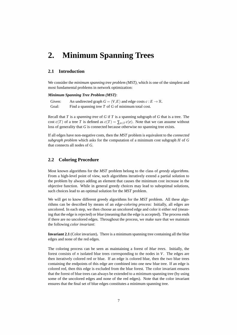
Assume that in stept we color an edgee using the blue rule. Ife∈ T, thenT satisfiesthe color invariant after stept and we are done. Otherwise,e /∈ T. Consider the cut(X, X) to which the blue rule is applied to colore= (u,v) (see Figure1). BecauseTis a spanning tree, there is a pathPuv in T that connects the endpointsu and v of e.At least one edge, saye′, of Puv must cross(X, X). Note thate′ cannot be red becauseT satisfies the color invariant. Alsoe′ cannot be blue because of the pre-conditions ofapplying the blue rule. Thus,e′ is uncolored and by the choice ofe, c(e) ≤ c(e′). Byremovinge′ from T and addinge, we obtain a new spanning treeT ′ = (T−e′)+eof costc(T ′) = c(T)− c(e′)+ c(e) ≤ c(T). Thus,T ′ is a minimum spanning tree that satisfiesthe color invariant after stept.
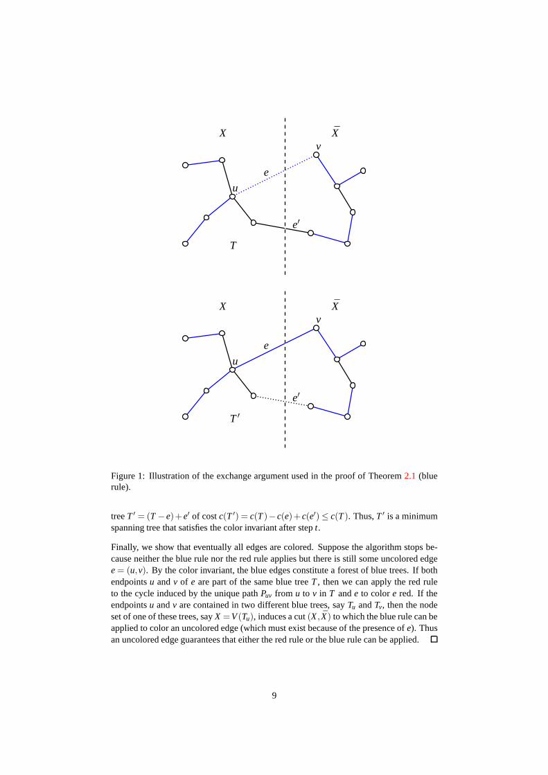
Assume that in stept we color an edgee using the red rule. Ife /∈ T, theT satisfies thecolor invariant after stept and we are done. Otherwise,e∈ T. Consider the cycleC towhich the red rule is applied to colore= (u,v) (see Figure2). By removinge from T, weobtain two trees whose node sets induce a cut(X, X). Note thatecrosses(X, X). BecauseC is a cycle, there must exist at least one other edge, saye′, in C that crosses(X, X). Notethate′ cannot be blue becausee′ /∈ T and the color invariant. Moreover,e′ cannot be redbecause of the pre-conditions of applying the red rule. Thus, e′ is uncolored and by thechoice ofe, c(e)≥ c(e′). By removinge from T and addinge′, we obtain a new spanning
8
T
X X
u
e
v
e′
T ′
X Xv
u
e
e′
Figure 1: Illustration of the exchange argument used in the proof of Theorem2.1 (bluerule).
treeT ′ = (T−e)+e′ of costc(T ′) = c(T)−c(e)+c(e′)≤ c(T). Thus,T ′ is a minimumspanning tree that satisfies the color invariant after stept.
Finally, we show that eventually all edges are colored. Suppose the algorithm stops be-cause neither the blue rule nor the red rule applies but thereis still some uncolored edgee= (u,v). By the color invariant, the blue edges constitute a forest of blue trees. If bothendpointsu andv of e are part of the same blue treeT, then we can apply the red ruleto the cycle induced by the unique pathPuv from u to v in T ande to colore red. If theendpointsu andv are contained in two different blue trees, sayTu andTv, then the nodeset of one of these trees, sayX =V(Tu), induces a cut(X, X) to which the blue rule can beapplied to color an uncolored edge (which must exist becauseof the presence ofe). Thusan uncolored edge guarantees that either the red rule or the blue rule can be applied.
9

T
X X
C
e′
u
e
v
T ′
X X
C
e′
u
e
v
Figure 2: Illustration of the exchange argument used in the proof of Theorem2.1 (redrule).
2.3 Kruskal’s Algorithm
Kruskal’s algorithm sorts the edges by non-decreasing costand then considers the edgesin this order. If the current edgeei = (u,v) has both its endpoints in the same blue tree, itis colored red; otherwise, it is colored blue. The algorithmis summarized in Algorithm1.
It is easy to verify that in each case the pre-conditions of the respective rule are met: Ifthe red rule applies, then the unique pathPuv in the blue tree containing both endpoints ofei together withei forms a cycleC. The edges inC∩Puv are blue andei is uncolored. Wecan thus apply the red rule toei . Otherwise, if the blue rule applies, thenei connects twoblue trees, sayTu andTv, in the current blue forest. Consider the cut(X, X) induced by thenode set ofTu, i.e.,X =V(Tu). No blue edge crosses this cut. Moreover,ei is an uncolorededge that crosses this cut. Also observe that every other uncolored edgee∈ δ (X) has cost
10

Input : undirected graphG= (V,E) with edge costsc : E→R
Output : minimum spanning treeT
1 Initialize: all edges are uncolored(Remark: we implicitly maintain a forest of blue trees below)
2 Let 〈e1, . . . ,em〉 be the list of edges ofG, sorted by non-decreasing cost3 for i← 1 to m do4 if ei has both endpoints in the same blue treethen colorei redelsecolorei
blue5 end6 Output the resulting treeT of blue edges
Algorithm 1: Kruskal’sMSTalgorithm.
c(e) ≥ c(ei) because we color the edges by non-decreasing cost. We can therefore applythe blue rule toei . An immediate consequence of Theorem2.1is that Kruskal’s algorithmcomputes a minimum spanning tree.
We next analyze the time complexity of the algorithm: The algorithm needs to sort theedges ofG by non-decreasing cost. There are different algorithms to do this with differentrunning times. The most efficient algorithms sort a list ofk elements inO(k logk) time.There is also a lower bound that shows that one cannot do better than that. That is, in ourcontext we spendΘ(mlogm) time to sort the edges by non-decreasing cost.
We also need to maintain a data structure in order to determine whether an edgeei has bothits endpoints in the same blue tree or not. A trivial implementation stores for each nodea unique identifier of the tree it is contained in. Checking whether the endpointsu andvof edgeei = (u,v) are part of the same blue tree can then be done inO(1) time. Mergingtwo blue trees needs timeO(n) in the worst case. Thus, the trivial implementation takesO(m+n2) time in total (excluding the time for sorting).
One can do much better by using a so-calledunion-finddata structure. This data struc-ture keeps track of the partition of the nodes into blue treesand allows only two types ofoperations:unionandfind. Thefind operation identifies the node set of the partition towhich a given node belongs. It can be used to check whether theendpointsu andv of edgeei = (u,v) belong to the same tree or not. Theunionoperation unites two node sets of thecurrent partition into one. This operation is needed to update the partition whenever wecolor ei = (u,v) blue and have to join the respective blue treesTu andTv. Sophisticatedunion-find data structures support a series ofn unionandm findoperations on a universeof n elements in timeO(n+mα(n, m
n )), whereα(n,d) is theinverse Ackerman function(see [8, Chapter 2] and the references therein).α(n,d) is increasing inn but grows ex-tremely slowly for every fixedd, e.g.,α(265536,0) = 4; for most practical situations, itcan be regarded as a constant.
The overall time complexity of Kruskal’s algorithm is thusO(mlogm+n+mα(n, mn )) =
O(mlogm) = O(mlogn) (think about it!).
Corollary 2.1. Kruskal’s algorithm solves the MST problem in time O(mlogn).
11

2.4 Prim’s Algorithm
Prim’s algorithm grows a single blue tree, starting at an arbitrary nodes∈ V. In everystep, it chooses among all edges that are incident to the current blue treeT containingsanuncolored edgeei of minimum cost and colors it blue. The algorithm stops ifT containsall nodes. We implicitly assume that all edges that are not part of the final tree are coloredred in a post-processing step. The algorithm is summarized in Algorithm2.
Input : undirected graphG= (V,E) with edge costsc : E→R
Output : minimum spanning treeT
1 Initialize: all edges are uncolored(Remark: we implicitly maintain a forest of blue trees below)
2 Choose an arbitrary nodes3 for i← 1 to n−1 do4 Let T be the current blue tree containings5 Select a minimum cost edgeei ∈ δ (V(T)) incident toT and color it blue6 end7 Implicitly: color all remaining edges red8 Output the resulting treeT of blue edges
Algorithm 2: Prim’s MSTalgorithm.
Note that the pre-conditions are met whenever the algorithmapplies one of the two col-oring rules: If the blue rule applies, then the node setV(T) of the current blue treeTcontainings induces a cut(X, X) with X = V(T). No blue edge crosses(X, X) by con-struction. Moreover,ei is among all uncolored edges crossing the cut one of minimumcost and can thus be colored blue. If the red rule applies to edgee= (u,v), both endpointsu andv are contained in the final treeT. The pathPuv in T together withe induce a cycleC. All edges inC∩Puv are blue and we can thus colore red.
The time complexity of the algorithm depends on how efficiently we are able to identifya minimum cost edgeei that is incident toT. To this aim, good implementations use apriority queuedata structure. The idea is to keep track of the minimum cost connectionsbetween nodes that are outside ofT to nodes inT. Suppose we maintain two data entriesfor every nodev /∈ V(T): π(v) = (u,v) refers to the edge that minimizesc(u,v) amongall u∈V(T) andd(v) = c(π(v)) refers to the cost of this edge; we defineπ(v) = nil andd(v) = ∞ if no such edge exists. Initially, we have for every nodev∈V \ s:
π(v) =
(s,v) if (s,v) ∈ E
nil otherwise.and d(v) =
c(s,v) if (s,v) ∈ E
∞ otherwise.
The algorithm now repeatedly chooses a nodev /∈ V(T) with d(v) minimum, adds it tothe tree and colors its connecting edgeπ(v) blue. Becausev is part of the new tree,we need to update the above data. This can be accomplished by iterating over all edges(v,w) ∈ E incident tov and verifying for every adjacent nodew with w /∈V(T) whetherthe connection cost fromw to T via edge(v,w) is less than the one stored ind(w) (viaπ(w)). If so, we update the respective data entries accordingly.Note that if the value of
12
d(w) changes, then it can only decrease.
There are several priority queue data structures that support all operations needed above:insert, find-min, delete-minanddecrease-priority. In particular, usingFibonacci heaps,m decrease-priorityandn insert/find-min/delete-minoperations can be performed in timeO(m+nlogn).
Corollary 2.2. Prim’s algorithm solves the MST problem in time O(m+nlogn).
References
The presentation of the material in this section is based on [8, Chapter 6].
13

3. Matroids
3.1 Introduction
In the previous section, we have seen that the greedy algorithm can be used to solve theMST problem. An immediate question that comes to ones mind iswhich other problemscan be solved by such an algorithm. In this section, we will see that the greedy algorithmapplies to a much broader class of optimization problems.
We first define the notion of anindependent set system.
Definition 3.1. Let Sbe a finite set and letI be a collection of subsets ofS. (S,I) is anindependent set systemif
(M1) /0∈ I ;(M2) if I ∈ I andJ⊆ I , thenJ ∈ I.
Each setI ∈ I is called anindependent set; every other subsetI ⊆ Swith I /∈ I is called adependent set. Further, suppose we are given a weight functionw : S→R on the elementsin S.
Maximum Weight Independent Set Problem (MWIS):
Given: An independent set system(S,I) and a weight functionw : S→R.Goal: Find an independent setI ∈ I of maximum weightw(I) = ∑x∈I w(x).
If w(x) < 0 for somex∈ S, thenx will not be included in any optimum solution becauseI is closed under taking subsets. We can thus safely exclude such elements from theground setS. Subsequently, we assume without loss of generality that all weights arenonnegative.
As an example, consider the following independent set system: Suppose we are givenan undirected graphG = (V,E) with weight functionw : E→ R+. DefineS= E andI = F ⊆ E | F induces a forest inG. Note that /0∈ I andI is closed under takingsubsets because each subsetJ of a forestI ∈ I is a forest. Now, the problem of finding anindependent setI ∈ I that maximizesw(I) is equivalent to finding a spanning tree ofGof maximum weight. (Note that the latter can also be done by one of the MST algorithmsthat we have considered in the previous section.)
The greedy algorithm given in Algorithm3 is a natural generalization of Kruskal’s algo-rithm to independent set systems. It starts with the empty set I = /0 and then iterativelyextendsI by always adding an elementx∈ S\ I of maximum weight, ensuring thatI + xremains an independent set.
Unfortunately, the greedy algorithm does not work for general independent set systemsas the following example shows:
14
Input : independent set system(S,I) with weight functionw : S→R
Output : independent setI ∈ I of maximum weight
1 Initialize: I = /0.2 while there is some x∈ S\ I with I + x∈ I do3 Choose such anx with w(x) maximum4 I ← I + x5 end6 return I
Algorithm 3: Greedy algorithm for matroids.
Example 3.1.
9
p s
q r
3
7
8
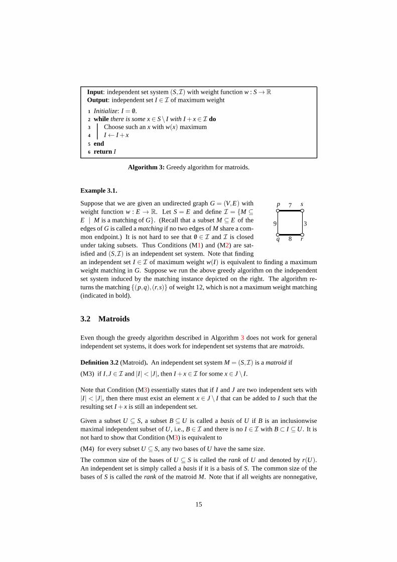
Suppose that we are given an undirected graphG = (V,E) withweight functionw : E → R. Let S= E and defineI = M ⊆E | M is a matching ofG. (Recall that a subsetM ⊆ E of theedges ofG is called amatchingif no two edges ofM share a com-mon endpoint.) It is not hard to see that /0∈ I andI is closedunder taking subsets. Thus Conditions (M1) and (M2) are sat-isfied and(S,I) is an independent set system. Note that findingan independent setI ∈ I of maximum weightw(I) is equivalent to finding a maximumweight matching inG. Suppose we run the above greedy algorithm on the independentset system induced by the matching instance depicted on the right. The algorithm re-turns the matching(p,q),(r,s) of weight 12, which is not a maximum weight matching(indicated in bold).
3.2 Matroids
Even though the greedy algorithm described in Algorithm3 does not work for generalindependent set systems, it does work for independent set systems that arematroids.
Definition 3.2 (Matroid). An independent set systemM = (S,I) is amatroid if
(M3) if I ,J ∈ I and|I |< |J|, thenI + x∈ I for somex∈ J\ I .
Note that Condition (M3) essentially states that ifI andJ are two independent sets with|I | < |J|, then there must exist an elementx∈ J \ I that can be added toI such that theresulting setI + x is still an independent set.
Given a subsetU ⊆ S, a subsetB⊆ U is called abasisof U if B is an inclusionwisemaximal independent subset ofU , i.e.,B∈ I and there is noI ∈ I with B⊂ I ⊆U . It isnot hard to show that Condition (M3) is equivalent to
(M4) for every subsetU ⊆ S, any two bases ofU have the same size.
The common size of the bases ofU ⊆ S is called therank of U and denoted byr(U).An independent set is simply called abasisif it is a basis ofS. The common size of thebases ofS is called therank of the matroidM. Note that if all weights are nonnegative,
15

the MWIS problem is equivalent to finding a maximum weight basis of M.
We give some examples of matroids.
Example 3.2(Uniform matroid). One of the simplest examples of a matroid is the so-calleduniform matroid. Suppose we are given some setS and an integerk. Define theindependent setsI as the set of all subsets ofSof size at mostk, i.e.,I = I ⊆S | |I | ≤ k.It is easy to verify thatM = (S,I) is a matroid.M is also called thek-uniform matroid.
Example 3.3(Partition matroid). Another simple example of a matroid is thepartitionmatroid. SupposeS is partitioned intom setsS1, . . . ,Sm and we are givenm integersk1, . . . ,km. DefineI = I ⊆ S | |I ∩Si | ≤ ki for all 1≤ i ≤m. Conditions (M1) and(M2) are trivially satisfied. To see that Condition (M3) is satisfied as well, note that ifI ,J ∈ I and|I |< |J|, then there is somei (1≤ i ≤m) such that|J∩Si |> |I ∩Si | and thusadding any elementx ∈ Si ∩ (J \ I) to I maintains independence. Thus,M = (S,I) is amatroid.
Example 3.4(Graphic matroid). Suppose we are given an undirected graphG= (V,E).Let S= E and defineI = F ⊆ E | F induces a forest inG. We already argued abovethat Conditions (M1) and (M2) are satisfied. We next show that Conditions (M4) is satis-fied too. LetU ⊆ E. Consider the subgraph(V,U) of G induced byU and suppose that itconsists ofk components. By definition, each basisB of U is an inclusionwise maximalforest contained inU . Thus,B consists ofk spanning trees, one for each component ofthe subgraph(V,U). We conclude thatB contains|V|− k elements. Because this holdsfor every basis ofU , Condition (M4) is satisfied. We remark that any matroidM = (S,I)obtained in this way is also called agraphic matroid(or cycle matroid).
Example 3.5(Matching matroid). The independent set system of Example3.1 is not amatroid. However, there is another way of defining a matroid based on matchings. LetG = (V,E) be an undirected graph. Given a matchingM ⊆ E of G, let V(M) refer tothe set of nodes that are incident to the edges ofM. A node setI ⊆ V is coveredbyM if I ⊆ V(M). DefineS= V andI = I ⊆ V | I is covered by some matchingM.Condition (M1) holds trivially. Condition (M2) is satisfied because if a node setI ∈ I iscovered by a matchingM, then each subsetJ⊆ I is also covered byM and thusJ ∈ I. Itcan also be shown that Condition (M3) is satisfied and thusM = (S,I) is a matroid.M isalso called amatching matroid.
3.3 Greedy Algorithm for Matroids
The next theorem shows that the greedy algorithm given in Algorithm3 always computesa maximum weight independent set if the underlying independent set system is a ma-troid. The theorem actually shows something much stronger:Matroids are precisely theindependent set systems for which the greedy algorithm computes an optimal solution.
Theorem 3.1. Let (S,I) be an independent set system. Further, let w: S→ R+ be anonnegative weight function on S. The greedy algorithm (Algorithm3) computes an inde-pendent set of maximum weight if and only if M= (S,I) is a matroid.
16

Proof. We first show that the greedy algorithm computes a maximum weight independentset if M is a matroid. LetX be the independent set returned by the greedy algorithm andlet Y be a maximum weight independent set. Note that bothX andY are bases ofM.Order the elements inX = x1, . . . ,xm such thatxi (1≤ i ≤m) is thei-th element chosenby the algorithm. Clearly,w(x1) ≥ ·· · ≥ w(xm). Also orderY = y1, . . . ,ym such thatw(y1)≥ ·· · ≥w(ym). We will show thatw(xi)≥w(yi) for everyi. Letk+1 be the smallestinteger such thatw(xk+1)< w(yk+1). (The claim follows if no such choice exists.) DefineI = x1, . . . ,xk andJ = y1, . . . ,yk+1. BecauseI ,J ∈ I and|I | < |J|, Condition (M3)implies that there is someyi ∈ J \ I such thatI + yi ∈ I. Note thatw(yi) ≥ w(yk+1) >
w(xk+1). That is, in iterationk+1, the greedy algorithm would prefer to addyi instead ofxk+1 to extendI , which is a contradiction. We conclude thatw(X)≥w(Y) and thusX is amaximum weight independent set.
Next assume that the greedy algorithm always computes an independent set of maximumweight for every independent set system(S,I) and weight functionw : S→ R+. Weshow thatM = (S,I) is a matroid. Conditions (M1) and (M2) is satisfied by assumption.It remains to show that Condition (M3) holds. LetI ,J ∈ I with |I |< |J| and assume, forthe sake of a contradiction, thatI + x /∈ I for everyx∈ J\ I . Let k= |I | and consider thefollowing weight function onS:
w(x) =
k+2 if x∈ I
k+1 if x∈ J\ I
0 otherwise.
Now, in the firstk iterations, the greedy algorithms picks the elements inI . By assumption,the algorithm cannot add any other element fromJ\ I and thus outputs a solution of weightk(k+2). However, the independent setJ has weight at least|J|(k+1)≥ (k+1)(k+1)>k(k+2). That is, the greedy algorithm does not compute a maximum weight independentset, which is a contradiction.
References
The presentation of the material in this section is based on [2, Chapter 8] and [7, Chapters39 & 40].
17

4. Shortest Paths
4.1 Introduction
We next consider shortest path problems. These problems areusually defined fordirectednetworks. Let G = (V,E) be a directed graph with cost functionc : E→ R. Consider a(directed) pathP= 〈v1, . . . ,vk〉 from s= v1 to t = vk. The lengthof pathP is defined asc(P) = ∑k−1
i=1 c(vi ,vi+1). We can then ask for the computation of ans, t-path whose lengthis shortest among all directed paths froms to t. There are different variants of shortestpath problems:
1. Single source single target shortest path problem: Given two nodessandt, deter-mine a shortest path froms to t.
2. Single source shortest path problem: Given a nodes, determine all shortest pathsfrom s to every other node inV.
3. All-pairs shortest path problem: For every pair(s, t) ∈V×V of nodes, compute ashortest path froms to t.
The first problem is a special case of the second one. However,every known algorithm forthe first problem implicitly also solves the second one (at least partially). We thereforefocus here on thesingle source shortest path problemand theall-pairs shortest pathproblem.
4.2 Single Source Shortest Path Problem
We consider the following problem:
Single Source Shortest Path Problem (SSSP):
Given: A directed graphG= (V,E) with cost functionc : E→ R and a sourcenodes∈V.
Goal: Compute a shortest path froms to every other nodev∈V.
Note that a shortest path froms to a nodev might not necessarily exist because of thefollowing two reasons: First,v might not be reachable fromsbecause there is no directedpath froms to v in G. Second, there might be arbitrarily short paths froms to v becauseof the existence of ans,v-path that contains a cycle of negative length (which can betraversed arbitrarily often). We call a cycle of negative total length also anegative cycle.The following lemma shows that these are the only two cases inwhich no shortest pathexists.
Lemma 4.1. Let v be a node that is reachable from s. Further assume that there is nopath from s to v that contains a negative cycle. Then there exists a shortest path from s tov which is a simple path.
Proof. Let P be a path froms to v. We can repeatedly remove cycles fromP until weobtain a simple pathP′. By assumption, all these cycles have non-negative lengthsand
18
thusc(P′) ≤ c(P). It therefore suffices to show that there is a shortest path among allsimples,v-paths. But this is obvious because there are only finitely many simple pathsfrom s to v in G.
4.2.1 Basic properties of shortest paths
We define adistance functionδ : V→R as follows: For everyv∈V,
δ (v) = infc(P) | P is a path froms to v.
With the above lemma, we have
δ (v) = ∞ if there is no path froms to vδ (v) = −∞ if there is a path froms to v that contains a negative cycleδ (v) ∈ R if there is a shortest (simple) path froms to v.
The next lemma establishes thatδ satisfies the triangle inequality.
Lemma 4.2. For every edge e= (u,v) ∈ E, we haveδ (v)≤ δ (u)+ c(u,v).
Proof. Clearly, the relation holds ifδ (u) = ∞. Supposeδ (u) =−∞. Then there is a pathP from s to u that contains a negative cycle. By appending edgee to P, we obtain a pathfrom s to v that contains a negative cycle and thusδ (v) = −∞. The relation again holds.Finally, assumeδ (u)∈R. Then there is a pathP from s to u of lengthδ (u). By appendingedgee to P, we obtain a path froms to v of lengthδ (u)+ c(u,v). A shortest path fromsto v can only have shorter length and thusδ (v)≤ δ (u)+ c(u,v).
The following lemma shows that subpaths of shortest paths are shortest paths.
Lemma 4.3. Let P= 〈v1, . . . ,vk〉 be a shortest path from v1 to vk. Then every subpathP′ = 〈vi , . . . ,v j〉 of P with1≤ i ≤ j ≤ k is a shortest path from vi to vj .
Proof. Suppose there is a pathP′′ = 〈vi ,u1, . . . ,ul ,v j〉 from vi to v j that is shorter thanP′.Then the path〈v1, . . . ,vi ,u1, . . . ,ul ,v j , . . . ,vk〉 is av1,vk-path that is shorter thanP, whichis a contradiction.
Consider a shortest pathP= 〈s= v1, . . . ,vk = v〉 from s to v. The above lemma enablesus to show that every edgee= (vi ,vi+1) of P must betight with respect to the distancefunctionδ , i.e.,δ (v) = δ (u)+ c(u,v).
Lemma 4.4. Let P= 〈s, . . . ,u,v〉 be a shortest s,v-path. Thenδ (v) = δ (u)+ c(u,v).
Proof. By Lemma4.3, the subpathP′ = 〈s, . . . ,u〉 of P is a shortests,u-path and thusδ (u) = c(P′). BecauseP is a shortests,v-path, we haveδ (v) = c(P) = c(P′)+ c(u,v) =δ (u)+ c(u,v).
19

Suppose now that we can computeδ (v) for every nodev∈V. Using the above lemmas, itis not difficult to show that we can then also efficiently determine the shortest paths froms to every nodev∈V with δ (v) ∈R: LetV ′ = v∈V | δ (v) ∈R be the set of nodes forwhich there exists a shortest path froms. Note thatδ (s) = 0 and thuss∈V ′. Further, letE′ be the set of edges that are tight with respect toδ , i.e.,
E′ = (u,v) ∈ E | δ (v) = δ (u)+ c(u,v).
Let G′ = (V ′,E′) be the subgraph ofG induced byV ′ and E′. Observe that we canconstructG′ in time O(n+m). By Lemma4.4, every edge of a shortest path froms tosome nodev∈ V ′ is tight. Thus every nodev∈V ′ is reachable froms in G′. Consider apathP= 〈s= v1, . . . ,vk = v〉 from s to v in G′. Then
c(P) =k−1
∑i=1
c(vi ,vi+1) =k−1
∑i=1
(δ (vi+1)− δ (vi)) = δ (v)− δ (s) = δ (v).
That is,P is a shortest path froms to v in G. G′ therefore represents all shortest paths froms to nodesv∈V ′. We can now extract a spanning treeT from G′ that is rooted ats, e.g.,by performing a depth-first search froms. Such a tree can be computed in timeO(n+m).Observe thatT contains for every nodev∈V ′ a uniques,v-path which is a shortest pathin G. T is therefore also called ashortest-path tree. Note thatT is a very compact way tostore for every nodev∈ V ′ a shortest path froms to v. This tree needsO(n) space only,while listing all these paths explicitly may needO(n2) space.
In light of the above observations, we will subsequently concentrate on the problem ofcomputing the distance functionδ efficiently. To this aim, we introduce a functiond :V → R of tentativedistances. The algorithm will used to compute a more and morerefined approximation ofδ until eventuallyd(v) = δ (v) for everyv ∈ V. We initialized(s) = 0 andd(v) = ∞ for everyv∈V \ s. The only operation that is used to modifydis to relax an edgee= (u,v) ∈ E:
RELAX(u,v):if d(v)> d(u)+ c(u,v) then d(v) = d(u)+ c(u,v)
It is obvious that thed-values can only decrease by edge relaxations.
We show that if we only relax edges then the tentative distances will never be less thanthe actual distances.
Lemma 4.5. For every v∈V, d(v)≥ δ (v).
Proof. The proof is by induction on the number of relaxations. The claim holds afterthe initialization becaused(v) = ∞ ≥ δ (v) andd(s) = 0= δ (s). For the induction step,suppose that the claim holds true before the relaxation of anedgee= (u,v). We showthat it remains valid after edgee has been relaxed. By relaxing(u,v), only d(v) can bemodified. If d(v) is modified, then after the relaxation we haved(v) = d(u)+ c(u,v) ≥δ (u) + c(u,v) ≥ δ (v), where the first inequality follows from the induction hypothesisand the latter inequality holds because of the triangle inequality (Lemma4.2).
20

That is,d(v) decreases throughout the execution but will never be lower than the actualdistanceδ (v). In particular,d(v) = δ (v) = ∞ for all nodesv∈ V that are not reachablefrom s. Our goal will be to use only few edge relaxations to ensure that d(v) = δ (v) foreveryv∈V with δ (v) ∈ R.
Lemma 4.6. Let P= 〈s, . . . ,u,v〉 be a shortest s,v-path. If d(u) = δ (u) before the relax-ation of edge e= (u,v), then d(v) = δ (v) after the relaxation of edge e.
Proof. Note that after the relaxation of edgee, we haved(v) = d(u)+ c(u,v) = δ (u)+c(u,v) = δ (v), where the last equality follows from Lemma4.4.
4.2.2 Arbitrary cost functions
The above lemma makes it clear what our goal should be. Namely, ideally we shouldrelax the edges ofG in the order in which they appear on shortest paths. The dilemma, ofcourse, is that we do not know these shortest paths. The following algorithm, also knownas theBellman-Fordalgorithm, circumvents this problem by simply relaxing every edgeexactlyn−1 times, thereby also relaxing all edges along shortest pathin the right order.An illustration is given in Figure4.
Input : directed graphG= (V,E), cost functionc : E→R, source nodes∈VOutput : shortest path distancesd : V→ R
1 Initialize: d(s) = 0 andd(v) = ∞ for everyv∈V \ s2 for i← 1 to n−1 do3 foreach(u,v) ∈ E do RELAX(u,v)4 end5 return d
Algorithm 4: Bellman-Ford algorithm for the SSSP problem.
Lemma 4.7. After the Bellman-Ford algorithm terminates, d(v) = δ (v) for all v∈V withδ (v)>−∞.
Proof. As argued above, after the initialization we haved(v) = δ (v) for all v∈ V withδ (v) =∞. Consider a nodev∈V with δ (v)∈R. LetP= 〈s= v1, . . . ,vk = v〉 be a shortests,v-path. Define aphaseof the algorithm as the execution of the inner loop. That is, thealgorithm consists ofn−1 phases and in each phase every edge ofG is relaxed exactlyonce. Note thatd(s) = δ (s) after the initialization. Using induction oni and Lemma4.6,we can show thatd(vi+1) = δ (vi+1) at the end of phasei. Thus, after at mostn−1 phasesd(v) = δ (v) for everyv∈V with δ (v) ∈ R.
Note that the algorithm does not identify nodesv ∈ V with δ (v) = −∞. However, thiscan be accomplished in a post-processing step (see exercises). The time complexity ofthe algorithm is obviouslyO(nm). Clearly, we might improve on this by stopping thealgorithm as soon as all tentative distances remain unchanged in a phase. However, thisdoes not improve on the worst case running time.
21

0
s
∞ ∞
∞ ∞
6
7
5
−2
−4
8
9
−3
7
2
0
s
6 11
7 2
6
7
5
−2
−4
8
9
−3
7
2
0
s
6 4
7 2
6
7
5
−2
−4
8
9
−3
7
2
0
s
2 4
7 −2
6
7
5
−2
−4
8
9
−3
7
2
Figure 3: Illustration of the Bellman-Ford algorithm. The order in which the edges arerelaxed in this example is as follows: We start with the upperright node and proceed ina clockwise order. For each node, edges are relaxed in clockwise order. Tight edges areindicated in bold. Only the first three phases are depicted (no change in the final phase).
Theorem 4.1. The Bellman-Ford algorithm solves the SSSP problem withoutnegativecycles in timeΘ(nm).
4.2.3 Nonnegative cost functions
The running time ofO(nm) of the Bellman-Ford algorithm is rather large. We can signif-icantly improve upon this in certain special cases. The easiest such special case is if thegraphG is acyclic.
Another example is if the edge costs are nonnegative. Subsequently, we assume that thecost functionc : E→R+ is nonnegative.
The best algorithm for the SSSP with nonnegative cost functions is known asDijkstra’salgorithm. As before, the algorithm starts withd(s) = 0 andd(v) = ∞ for everyv ∈V \s. It also maintains a setV∗ of nodes whose distances are tentative. Initially,V∗=V.The algorithm repeatedly chooses a nodeu ∈ V∗ with d(u) minimum, removes it fromV∗ and relaxes all outgoing edges(u,v). The algorithm stops whenV∗ = /0. A formaldescription is given in Algorithm5.
Note that the algorithm relaxes every edge exactly once. Intuitively, the algorithm canbe viewed as maintaining a “cloud” of nodes (V \V∗) whose distance labels are exact. Ineach iteration, the algorithm chooses a nodeu∈V∗ that is closest to the cloud, declares itsdistance label as exact and relaxes all its outgoing edges. As a consequence, other nodesoutside of the cloud might get closer to the cloud. An illustration of the execution of thealgorithm is given in Figure4.
22

Input : directed graphG= (V,E), nonnegative cost functionc : E→R, source nodes∈V
Output : shortest path distancesd : V→ R
1 Initialize: d(s) = 0 andd(v) = ∞ for everyv∈V \ s2 V∗ =V3 while V∗ 6= /0 do4 Choose a nodeu∈V∗ with d(u) minimum.5 Removeu fromV∗.6 foreach(u,v) ∈ E do RELAX(u,v)7 end8 return d
Algorithm 5: Dijkstra’s algorithm for the SSSP problem.
The correctness of the algorithm follows from the followinglemma.
Lemma 4.8. Whenever a node u is removed from V∗, we have d(u) = δ (u).
Proof. The proof is by contradiction. Consider the first iteration in which a nodeu isremoved fromV∗ while d(u)> δ (u). Let A⊆V be the set of nodesv with d(v) = δ (v).Note thatu is reachable froms becauseδ (u) < ∞. Let P be a shortests,u-path. If wetraverseP from s to u, then there must be an edge(x,y) ∈ P with x∈ A andy /∈ A becauses∈A andu /∈A. Let(x,y) be the first such edge onP. We haved(x)= δ (x)≤ δ (u)< d(u),where the first inequality holds because all edge costs are nonnegative. Consequently,xwas removed fromV∗ beforeu. By the choice ofu, d(x) = δ (x) whenx was removedfromV∗. But then, by Lemma4.6, we must haved(y) = δ (y) after the relaxation of edge(x,y), which is a contradiction to the assumption thaty /∈ A.
The running time of Dijkstra’s algorithm crucially relies on the underlying data structure.An efficient way to keep track of the tentative distance labels and the setV∗ is to usepriority queues. We need at mostn insert(initialization),n delete-min(removing nodeswith minimumd-value) andm decrease-priorityoperations (updating distance labels afteredge relaxations).Fibonacci heapssupport these operations in timeO(m+nlogn).
Theorem 4.2. Dijkstra’s algorithm solves the SSSP problem with nonnegative edge costsin time O(m+nlogn).
4.3 All-pairs Shortest-path Problem
We next consider the following problem:
All-pairs Shortest Path Problem (APSP):
Given: A directed graphG= (V,E) with cost functionc : E→ R.Goal: Determine a shortests, t-path for every pair(s, t) ∈V×V.
23

0
s
∞ ∞
∞ ∞
10
5
2 3
1
2
9
4 6
2
0
s
10 ∞
5 ∞
10
5
2 3
1
2
9
4 6
2
0
s
8 14
5 7
10
5
2 3
1
2
9
4 6
2
0
s
8 13
5 7
10
5
2 3
1
2
9
4 6
2
0
s
8 9
5 7
10
5
2 3
1
2
9
4 6
2
0
s
8 9
5 7
10
5
2 3
1
2
9
4 6
2
Figure 4: Illustration of Dijsktra’s algorithm. The nodes in V \V∗ are depicted in gray.The current node that is removed fromV∗ is drawn in bold. The respective edge relax-ations are indicated in bold.
24

Input : directed graphG= (V,E), nonnegative cost functionc : E→ R
Output : shortest path distancesd : V×V→ R
1 Initialize: foreach(u,v) ∈V×V do d(u,v) =
0 if u= v
c(u,v) if (u,v) ∈ E
∞ otherwise.2 for k← 1 to n do3 foreach(u,v) ∈V×V do4 if d(u,v)> d(u,k)+d(k,v) then d(u,v) = d(u,k)+d(k,v)5 end6 end7 return d
Algorithm 6: Floyd-Warshall algorithm for the APSP problem.
We assume thatG contains no negative cycle.
Define a distance functionδ : V×V→ R as
δ (u,v) = infc(P) | P is a path fromu to v.
Note thatδ is not necessarily symmetric. As for the SSSP problem, we canconcentrateon the computation of the distance functionδ because the actual shortest paths can beextracted from these distances.
Clearly, one way to solve the APSP problem is to simply solven SSSP problems: Forevery nodes∈ V, solve the SSSP problem with source nodes to compute all distancesδ (s, ·). Using the Bellman-Ford algorithm, the worst-case runningtime of this algorithmis O(n2m), which for dense graphs isΘ(n4). We will see that we can do better.
The idea is based on a general technique to derive exact algorithms known asdynamicprogramming. Basically, the idea is to decompose the problem into smaller sub-problemswhich can be solved individually and to use these solutions to construct a solution for thewhole problem in a bottom-up manner.
Suppose the nodes inV are identified with the set1, . . . ,n. In order to define thedynamic program, we need some more notion. Consider a simpleu,v-pathP = 〈u =
v1, . . . ,vl = v〉. We call the nodesv2, . . . ,vl−1 the interior nodesof P; P has no interiornodes ifl ≤ 2. A u,v-pathP whose interior nodes are all contained in1, . . . ,k is calleda (u,v,k)-path. Define
δk(u,v) = infc(P) | P is a(u,v,k)-path
as the shortest path distance of a(u,v,k)-path. Clearly, with this definition we haveδ (u,v) = δn(u,v). Our task is therefore to computeδn(u,v) for everyu,v∈V.
Our dynamic program is based on the following observation. Suppose we are able tocomputeδk−1(u,v) for all u,v∈V. Consider a shortest(u,v,k)-pathP= 〈u= v1, . . . ,vl =
v〉. Note thatP is simple because we assume thatG contains no negative cycles. By
25

definition, the interior nodes ofP belong to the set1, . . . ,k. There are two cases thatcan occur: Either nodek is an interior node ofP or not.
First, assume thatk is not an interior node ofP. Then all interior nodes ofP must belongto the set1, . . . ,k− 1. That is,P is a shortest(u,v,k− 1)-path and thusδk(u,v) =δk−1(u,v).
Next, supposek is an interior node ofP, i.e.,P= 〈u= v1, . . . ,k, . . . ,vl = v〉. We can thenbreakP into two pathsP1 = 〈u, . . . ,k〉 andP2 = 〈k, . . . ,v〉. Note that the interior nodes ofP1 andP2 are contained in1, . . . ,k−1 becauseP is simple. Moreover, because subpathsof shortest paths are shortest paths, we conclude thatP1 is a shortest(u,k,k−1)-path andP2 is a shortest(k,v,k−1)-path. Therefore,δk(u,v) = δk−1(u,k)+ δk−1(k,v).
The above observations lead to the following recursive definition of δk(u,v):
δ0(u,v) =
0 if u= v
c(u,v) if (u,v) ∈ E
∞ otherwise.
andδk(u,v) = minδk−1(u,v), δk−1(u,k)+ δk−1(k,v) if k≥ 1
The Floyd-Warshall algorithm simply computesδk(u,v) in a bottom-up manner. Thealgorithm is given in Algorithm6.
Theorem 4.3. The Floyd-Warshall algorithm solves the APSP problem without negativecycles in timeΘ(n3).
References
The presentation of the material in this section is based on [3, Chapters 25 and 26].
26
5. Maximum Flows
5.1 Introduction
Themaximum flow problemis a fundamental problem in combinatorial optimization withmany applications in practice. We are given a network consisting of a directed graphG= (V,E) and nonnegative capacitiesc : E→ R+ on the edges and a source nodes∈Vand a target nodet ∈V.
Intuitively, think of G being a water network and suppose that we want to send as muchwater as possible (say per second) from a source nodes (producer) to a target nodet(consumer). An edge ofG corresponds to a pipeline of the water network. Every pipelinecomes with a capacity which specifies the maximum amount of water that can be sentthrough it (per second). Basically, themaximum flow problemasks how the water shouldbe routed through the network such that the total amount of water that can be sent fromsto t (per second) is maximized.
We assume without loss of generality thatG is complete. IfG is not complete, then wesimply add every missing edge(u,v) ∈ V ×V \E to G and definec(u,v) = 0. We alsoassume that every nodeu∈V lies on a path froms to t (other nodes will be irrelevant).
Definition 5.1. A flow (or s, t-flow) in G is a function f : V ×V → R that satisfies thefollowing three properties:
1. Capacity constraint: For all u,v∈V, f (u,v)≤ c(u,v).2. Skew symmetry: For allu,v∈V, f (u,v) =− f (v,u).3. Flow conservation: For everyu∈V \ s, t, we have
∑v∈V
f (u,v) = 0.
The quantityf (u,v) can be interpreted as thenet flowfrom u to v (which can be positive,zero or negative). The capacity constraint ensures that theflow value of an edge does notexceed the capacity of the edge. Note that skew symmetry expresses that the net flowf (u,v) that is sent fromu to v is equal to the net flowf (v,u) =− f (u,v) that is sent fromv to u. Also the total net flow fromu to itself is zero becausef (u,u) =− f (u,u) = 0. Theflow conservation constraints make sure that the total flow out of a nodeu∈V \ s, t iszero. Because of skew symmetry, this is equivalent to stating that the total flow intou iszero.
Another way of interpreting the flow conservation constraints is that the total positive netflow entering a nodeu∈V \ s, t is equal to the total positive net flow leavingu, i.e.,
∑v∈V: f (v,u)>0
f (v,u) = ∑v∈V: f (u,v)>0
f (u,v).
Thevalue| f | of a flow f refers to the total net flow out ofs (which by the flow conserva-
27

s
p q
u v
t
16
13
10 4
12
14
9
7
20
4
s
p q
u v
t
11
8
1
12
11
4
7
15
4
Figure 5: On the left: Input graphG with capacitiesc : E→ R+. Only the edges withpositive capacity are shown. On the right: A flowf of G with flow value| f | = 19. Onlythe edges with positive net flow are shown.
tion constraints is the same as the total flow intot):
| f |= ∑v∈V
f (s,v).
An example of a network and a flow is given in Figure5.
The maximum flow reads as follows:
Maximum Flow Problem:
Given: A directed graphG= (V,E) with capacitiesc : E→R+, a source nodes∈V and a destination nodet ∈V.
Goal: Compute ans, t-flow f of maximum value.
We introduce some more notation. Given two setsX,Y⊆V, define
f (X,Y) = ∑x∈X
∑y∈Y
f (x,y).
We state a few properties. (You should try to convince yourself that these properties holdtrue.)
Proposition 5.1. Let f be a flow in G. Then the following holds true:
1. For every X⊆V, f(X,X) = 0.2. For every X,Y ⊆V, f(X,Y) =− f (Y,X).3. For every X,Y,Z⊆V with X∩Y = /0,
f (X∪Y,Z) = f (X,Z)+ f (Y,Z) and f(Z,X∪Y) = f (Z,X)+ f (Z,Y).
5.2 Residual Graph and Augmenting Paths
Consider ans, t-flow f . Let theresidual capacityof an edgee= (u,v) ∈ E with respectto f be defined as
r f (u,v) = c(u,v)− f (u,v).
28

s
p q
u v
t
11
5
5
8
11 3
3
11
12
7
4
5
4
5
15
s
p q
u v
t
11
12
1
12
11
7
19
4
Figure 6: On the left: Residual graphGf with respect to the flowf given in Figure5. Anaugmenting pathP with r f (P) = 4 is indicated in bold. On the right: The flowf ′ obtainedfrom f by augmentingr f (P) units of flow alongP. Only the edges with positive flow areshown. The flow value off ′ is | f ′|= 23. (Note thatf ′ is optimal because the cut(X, X)of G with X = q, t has capacityc(X, X) = 23.)
Intuitively, the residual capacityr f (u,v) is the amount of flow that can additionally besent fromu to v without exceeding the capacityc(u,v). Call an edgee∈ E a residualedgeif it has positive residual capacity and asaturatededge otherwise. Theresidualgraph Gf = (V,Ef ) with respect tof is the subgraph ofG whose edge setEf consists ofall residual edges, i.e.,
Ef = e∈ E | r f (e)> 0.
See Figure6 (left) for an example.
Lemma 5.1. Let f be a flow in G. Let g be a flow in the residual graph Gf respectingthe residual capacities rf . Then the combined flow h= f + g is a flow in G with value|h|= | f |+ |g|.
Proof. We show that all properties of Definition5.1are satisfied.
First,h satisfies the skew symmetry property because for everyu,v∈V
h(u,v) = f (u,v)+g(u,v) =−( f (v,u)+g(v,u)) =−h(v,u).
Second, observe that for everyu,v∈V, g(u,v)≤ r f (u,v) and thus
h(u,v) = f (u,v)+g(u,v)≤ f (u,v)+ r f (u,v) = f (u,v)+ (c(u,v)− f (u,v)) = c(u,v).
That is, the capacity constraints are satisfied.
Finally, we have for everyu∈V \ s, t
∑v∈V
h(u,v) = ∑v∈V
f (u,v)+ ∑v∈V
g(u,v) = 0
and thus flow conservation is satisfied too.
29

Similarly, we can show that
|h|= ∑v∈V
h(s,v) = ∑v∈V
f (s,v)+ ∑v∈V
g(s,v) = | f |+ |g|.
An augmenting pathis a simples, t-pathP in the residual graphGf . Let P be an aug-menting path inGf . All edges ofP are residual edges. Thus, there exists somex> 0 suchthat we can sendx flow units additionally alongP without exceeding the capacity of anyedge. In fact, we can choosex to be as large as theresidual capacity rf (P) of P which isdefined as
r f (P) = minr f (u,v) | e∈ P.
Note that if we increase the flow of an edge(u,v) ∈ P by x = r f (P), then we also haveto decrease the flow value on(v,u) by x because of the skew symmetry property. We willalso say that weaugment the flow f along path P. See Figure6 for an example.
Lemma 5.2. Let f be a flow in G and let P be an augmenting path in Gf . Then f′ :V×V→ R with
f ′(u,v) =
f (u,v)+ r f (P) if (u,v) ∈ P
f (u,v)− r f (P) if (v,u) ∈ P
f (u,v) otherwise
is a flow in G of value| f ′|= | f |+ r f (P).
Proof. Observe thatf ′ can be decomposed into the original flowf and a flow fP thatsendsr f (P) units of flow alongP and−r f (P) flow units along thereversedpath ofP, i.e.,the path that we obtain fromP if we reverse the direction of every edgee∈ P. Clearly, fPis a flow inGf of valuer f (P). By Lemma5.1, the combined flowf ′ = f + fP is a flow inG of value| f ′|= | f |+ r f (P).
5.3 Ford-Fulkerson Algorithm
The observations above already suggest a first algorithm forthe max-flow problem: Ini-tialize f to be the zero flow, i.e.,f (u,v) = 0 for all u,v∈V. Let Gf be the residual graphwith respect tof . If there exists an augmenting pathP in the residual graphGf , thenaugmentf alongP and repeat; otherwise terminate. This algorithm is also known as theFord-Fulkersonalgorithm and is summarized in Algorithm7.
Note that it is not clear that the algorithm terminates nor that the computed flow is ofmaximum value. The correctness of the algorithm will followfrom themax-cut min-flowtheorem(Theorem5.3) discussed in the next section.
The running time of the algorithm depends on the number of iterations that we needto perform. Every single iteration can be implemented to runin time O(m). If all edgecapacities are integral, then it is easy to see that after each iteration the flow value increasesby at least one. The total number of iterations is therefore at most | f ∗|, where f ∗ is a
30

Input : directed graphG= (V,E), capacity functionc : E→R+, source anddestination nodess, t ∈V
Output : maximum flow f : V×V→R
1 Initialize: f (u,v) = 0 for everyu,v∈V2 while there exists an augmenting path P in Gf do3 augment flowf alongP4 end5 return f
Algorithm 7: Ford-Fulkerson algorithm for the max-flow problem.
maximum flow. Note that we can also handle the case when each capacity is a rationalnumber by scaling all capacities by a suitable integerD. However, note that the worst caserunning time of the Ford-Fulkerson algorithm can be prohibitively large. An instance onwhich the algorithm admits a bad running time is given in Figure7.
Theorem 5.1. The Ford-Fulkerson algorithm solves the max-flow problem with integercapacities in time O(m| f ∗|), where f∗ is a maximum flow.
Ford and Fulkerson gave an instance of the max-flow problem that shows that for irrationalcapacities the algorithm might fail to terminate.
Note that if all capacities are integers then the algorithm maintains an integral flow. Thatis, the Ford-Fulkerson also gives an algorithmic proof of the following integrality prop-erty.
Theorem 5.2(Integrality property). If all capacities are integral, then there is an integermaximum flow.
5.4 Max-Flow Min-Cut Theorem
A cut (or s, t-cut) of G is a partition of the node setV into two sets:X andX =V \X suchthats∈ X andt ∈ X. Recall thatG is directed. Thus, there are two types of edges crossingthe cut(X, X), namely the ones that leaveX and the ones that enterX. As for flows, itwill be convenient to define forX,Y ⊆V,
c(X,Y) = ∑u∈X
∑v∈Y
c(u,v).
Thecapacityof a cut(X, X) is defined as the total capacityc(X, X) of the edges leavingX. Fix an arbitrary flowf in G and consider an an arbitrary cut(X, X) of G. The total netflow leavingX is | f |.
Lemma 5.3. Let f be a flow and let(X, X) be a cut of G. Then the net flow leaving X isf (X, X) = | f |.
31

s
p
u
t
B
B
B
1
B
s
p
u
t
1
1
1 s
p
u
t
1
1
1
1
Figure 7: A bad instance for the Ford-Fulkerson algorithm (left). Suppose thatB is alarge integer. The algorithm alternately augments one unitof flow along the two paths〈s,u, p, t〉 and〈s, p,u, t〉. The flow after two augmentations is shown on the right. Thealgorithm needs 2B augmentations to find a maximum flow.
Proof.
f (X,V \X) = f (X,V)− f (X,X) = f (X,V) = f (s,V)+ f (X− s,V) = f (s,V) = | f |.
Intuitively, it is clear that if we consider an arbitrary cut(X, X) of G, then the total flowf (X, X) that leavesX is at mostc(X, X). The next lemma shows this formally.
Lemma 5.4. The flow value of any flow f in G is at most the capacity of any cut(X, X)
of G, i.e., f(X, X)≤ c(X, X).
Proof. By Lemma5.3, we have
| f |= f (X, X) = ∑u∈X
∑v∈V\X
f (u,v) ≤ ∑u∈X
∑v∈V\X
c(u,v) = c(X, X).
A fundamental result for flows is that the value of a maximum flow is equal to the mini-mum capacity of a cut.
Theorem 5.3(Max-Flow Min-Cut Theorem). Let f be a flow in G. Then the followingconditions are equivalent:
1. f is a maximum flow of G.2. The residual graph Gf contains no augmenting path.3. | f |= c(X, X) for some cut(X, X) of G.
Proof. (1)⇒ (2): Suppose for the sake of contradiction thatf is a maximum flow ofGand there is an augmenting pathP in Gf . By Lemma5.2, we can augmentf alongP andobtain a flow of value strictly larger than| f |, which is a contradiction.
(2)⇒ (3): Suppose thatGf contains no augmenting path. LetX be the set of nodes thatare reachable froms in Gf . Note thatt /∈ X because there is no path froms to t in Gf .That is,(X, X) is a cut ofG. By Lemma5.3, | f | = f (X, X). Moreover, for everyu∈ Xandv∈ X, we must havef (u,v) = c(u,v) because otherwise(u,v) ∈ Ef andv would bepart ofX. We conclude| f |= f (X, X) = c(X, X).
32
(3)⇒ (1): By Lemma5.4, the value of any flow is at most the capacity of any cut. Thecondition| f |= c(X, X) thus implies thatf is a maximum flow. (Also note that this impliesthat(X, X) must be a cut of minimum capacity.)
5.5 Edmonds-Karp Algorithm
The Edmonds-Karp Algorithm works almost identical to the Ford-Fulkerson algorithm.The only difference is that it chooses in each iteration ashortestaugmenting path inthe residual graphGf . An augmenting path is ashortestaugmenting path if it has theminimum number of edges among all augmenting paths inGf . The algorithm is given inAlgorithm 8.
Input : directed graphG= (V,E), capacity functionc : E→R+, source anddestination nodess, t ∈V
Output : maximum flow f : V×V→R
1 Initialize: f (u,v) = 0 for everyu,v∈V2 while there exists an augmenting path in Gf do3 determine a shortest augmenting pathP in Gf
4 augmentf alongP5 end6 return f
Algorithm 8: Edmonds-Karp algorithm for the max-flow problem.
Note that each iteration can still be implemented to run in timeO(m). A shortest augment-ing path inGf can be found by using a breadth-first search algorithm. As we will show,this small change makes a big difference in terms of the running time of the algorithm.
Theorem 5.4. The Edmonds-Karp algorithm solves the max-flow problem in timeO(nm2).
Note that the correctness of the Edmonds-Karp algorithm follows from the max-flowmin-cut theorem: The algorithm halts when there is not augmenting path inGf . ByTheorem5.3, the resulting flow is a maximum flow. It remains to show that the algorithmterminates afterO(nm) iterations. The crucial insight in order to prove this is that theshortest path distance of a node can only increase as the algorithm progresses.
Fix an arbitrary iteration of the algorithm. Letf be the flow at the beginning of the itera-tion and letf ′ be the flow at the end of the iteration. We obtainf ′ from f by augmentingf along an augmenting pathP in Gf . Further,P must be a shortest augmenting path inGf . Let P= 〈s= v0, . . . ,vk = t〉. We define two distance functions (in terms of number ofedges on a path): Letδ (u,v) be the number of edges on a shortest path fromu to v in Gf .Similarly, letδ ′(u,v) be the number of edges on a shortest path fromu to v in Gf ′ .
Note thatδ (s,vi) = i. Also observe that if an edge(u,v) is part of Gf ′ but not partof Gf , thenu = vi andv = vi−1 for somei. To see this observe thatf (u,v) = c(u,v)because(u,v) /∈ Ef . On the other hand,f ′(u,v)< c(u,v) because(u,v) ∈ Ef ′ . That is, by
33
augmentingf alongP, the flow on edge(u,v) was decreased. That means that the flowon the reverse edge(v,u) was increased and thus(v,u) must be part ofP.
The next lemma shows that for every nodev∈ V, the shortest path distance froms to vdoes not decrease.
Lemma 5.5. For each v∈V, δ ′(s,v)≥ δ (s,v).
Proof. Suppose there exists a nodev with δ ′(s,v) < δ (s,v). Among all such nodes, letv be one withδ ′(s,v) being smallest. Note thatv 6= s becauseδ (s,s) = δ ′(s,s) = 0 bydefinition. LetP′ be a shortests,v-path inGf ′ of distanceδ ′(s,v) and letu be the second-last node ofP′. BecauseP′ is a shortest path and by the choice ofv, we have
δ (s,v)> δ ′(s,v) = δ ′(s,u)+1≥ δ (s,u)+1. (5)
Note that the distance functionδ satisfies the triangle inequality. Therefore, edge(u,v)cannot be part ofGf because otherwise we would haveδ (s,v)≤ δ (s,u)+1. That is,(u,v)is contained inGf ′ but not contained inGf . Using our observation above, we concludethat there is somei (1≤ i ≤ k) such thatu= vi andv= vi−1. But thenδ (s,v) = i−1 andδ (s,u) = i which is a contradiction to (5).
Consider an augmentation of the current flowf along pathP. We say that an edgee=
(u,v) is critical with respect tof andP if (u,v) is part of the augmenting pathP and itsresidual capacity coincides with the amount of flow that is pushed alongP, i.e.,r f (u,v) =r f (P). Note that after the augmentation off alongP, every critical edge onP will besaturated and thus vanishes from the residual network.
Lemma 5.6. The number of times an edge e= (u,v) is critical throughout the executionof the algorithm is bounded by O(n).
Proof. Suppose edgee= (u,v) is critical with respect to flowf and pathP. Let δ referto the shortest path distances inGf . We have
δ (s,v) = δ (s,u)+1.
After the augmentation off alongP, edgee is saturated and thus disappears from theresidual graph. It can only reappear in the residual graph when in a successive iterationsome positive flow is pushed over the reverse edge(v,u). Suppose edge(v,u) is part of anaugmenting pathP′ that is used to augment the current flow, sayf ′. Letδ ′ be the distancefunction with respect toGf ′ . We have
δ ′(s,u) = δ ′(s,v)+1.
By Lemma5.5, δ (s,v) ≤ δ ′(s,v) and thus
δ ′(s,u) = δ ′(s,v)+1≥ δ (s,v)+1= δ (s,u)+2.
That is, between any two augmentations for which edgee= (u,v) is critical, the distanceof u from smust increases by at least 2.
34

Note that the distance ofu from s is at least 0 initially and can never be more thann−2.The number of times edgee= (u,v) is critical is thus bounded byO(n).
The proof of Theorem5.4now follows trivially:
Proof of Theorem5.4. As argued above, the Edmonds-Karp algorithm computes a maxi-mum flow if it terminates. Note that in every iteration of the algorithm at least one edgeis critical. By Lemma5.6, every edge is at mostO(n) times critical. The number ofiterations is thus bounded byO(nm).
References
The presentation of the material in this section is based on [3, Chapter 27] and [2, Chapter3]
35

6. Minimum Cost Flows
6.1 Introduction
We consider theminimum cost flow problem.
Minimum Cost Flow Problem:
Given: A directed graphG= (V,E) with capacitiesw : E→ R+ and costsc :E→R+ and a balance functionb : V→R.
Goal: Compute a feasible flowf such that the overall cost∑e∈E c(e) f (e) isminimized.
Here, a flowf : E→R+ is said to befeasibleif it respects the capacity constraints and thetotal flow at every nodeu∈V is equal to the balanceb(u). More formally, f is feasible ifthe following two conditions are satisfied:
1. Capacity constraint: for every(u,v) ∈ E, f (u,v)≤ w(u,v).2. Flow balance constraints:for everyu∈V,
∑(u,v)∈E
f (u,v)− ∑(v,u)∈E
f (v,u) = b(u).
Intuitively, a positive balance indicates that nodeu has asupplyof b(u) units of flow,while a negative balance indicates that nodeu has ademandof −b(u) units of flow. Afeasible flowf that satisfies the flow balance constraints withb(u) = 0 for everyu∈V iscalled acirculation.
Theminimum cost flow problemcan naturally be formulated as a linear program:
minimize ∑e∈E
c(e) f (e)
subject to ∑(u,v)∈E
f (u,v)− ∑(v,u)∈E
f (v,u) = b(u) ∀u∈V
f (e) ≤ w(e) ∀e∈ Ef (e) ≥ 0 ∀e∈ E
(6)
We usec( f ) = ∑e∈E c(e) f (e) to refer to the total cost of a feasible flowf . We make a fewassumptions throughout this section:
Assumption 6.1. Capacities, costs and balances are integral.
Note that we can enforce this assumption if all input numbersare rational numbers bymultiplying by a suitably large constant.
Assumption 6.2. The balance function satisfies∑u∈V b(u) = 0 and there is a feasibleflow satisfying these balances.
Note that we can test whether a feasible flow exists by a singlemax-flow computationas follows: Augment the network by adding a super-sources and a super-targett. Add
36

p2
q−2
x
2
y
−2
1,1
2,1
2,1
1,1
(a)
s
p q
x y
t
2
2
1
1
1
1
2
2
(b)
Figure 8: (a) Minimum cost flow instance. Every edge(u,v) is labeled withc(u,v),w(u,v)and every nodeu is labeled withb(u). (b) Augmented network to test feasibility. Everyedge(u,v) is labeled withw(u,v).
an edge(s,u) for every nodeu∈V with b(u) > 0 of capacityw(s,u) = b(u). Similarly,add an edge(u, t) for every nodeu∈V with b(u)< 0 of capacityw(u, t) =−b(u). Now,compute a maximums, t-flow in the augmented network. It is not hard to see that thereis a feasible flow for the original instance if and only if the maximum flow saturates alledges out ofs (or, equivalently, intot).
Subsequently, letW = maxe∈E w(e) refer to the maximum capacity of an edge,C =
maxe∈E c(e) to the maximum edge cost andB= maxu∈V b(u) to the maximum balance.
6.2 Flow Decomposition and Residual Graph
We establish a few basic properties of flows and circulationsand introduce the importantconcept of residual graphs.
Lemma 6.1. Let f be circulation of G. Then f can be decomposed into at mostm= |E|directed simple cycle flows.
Proof. Let G+f = (V,E+
f ) be thesupport subgraphof G that contains all edges with posi-tive flow value with respect tof , i.e.,
E+f = e∈ E | f (e) > 0.
Consider an arbitrary directed simple cycleC in G+f . Let x be the smallest flow value of
an edge inC, i.e., x = mine∈C f (e). We can decomposef such thatf = f ′+ fC, wherefC(u,v) = x for every(u,v) ∈C and fC(u,v) = 0 otherwise. Note thatf ′ is a circulationand fC is a cycle flow. We can now repeat this procedure withf ′ instead off . Note thatat least one edgee of C must satisfyf ′(e) = 0 and thus vanishes from the support graphof f ′. After at mostm iterations, we therefore obtain a decomposition off consisting ofat mostm directed simple cycle flows.
As for the maximum flow problem, the concept of aresidual graphwill play a crucial
37

role: Supposef is a feasible flow ofG. We introduce for each edgee= (u,v) ∈ E thereverse edge(v,u) with costc(v,u) = −c(u,v). Subsequently, these edges will be calledbackward edges. In contrast, we refer to the original edges(u,v) ∈ E asforward edges.The residual capacityof a forward edge(u,v) is defined asr f (u,v) = w(u,v)− f (u,v).The residual capacity of a backward edge(v,u) is r f (v,u) = f (u,v). Theresidual graphGf = (V,Ef ) with respect tof is the graph that contains all edges with positive residualcapacity.
Consider a directed simple cycleC in the residual graphGf . Let theresidual capacityofC ber f (C) = mine∈C r f (e). We can then pushx= r f (C) additional units of flow alongCto obtain a feasible flowf ′. Observe that an increase ofx units on a backward edge(v,u)corresponds to a decrease ofx units on the forward edge(u,v) ∈ E. More formally, theflow f ′ that we obtain fromf by augmenting x units of flow along Cis defined as follows:for every edgee= (u,v) ∈ E, we have
f ′(u,v) =
f (u,v)+ x if (u,v) ∈C
f (u,v)− x if (v,u) ∈C
f (u,v) otherwise.
Let the total cost of a cycleC in Gf bec(C) = ∑e∈C c(e).
Lemma 6.2. Let f be a feasible flow of G and let C be a directed simple cycle in Gf .Suppose f′ is a flow that is obtained from f by augmenting x= r f (C) units of flow alongC. Then f′ is a feasible flow of G. Moreover, we have c( f ′) = c( f )+ x ·c(C).
Proof. Observe thatx ≤ r f (u,v) for every edge(u,v) ∈ C. If (u,v) ∈ C is a forwardedge, thenf ′(u,v) = f (u,v)+ x≤ f (u,v) +w(u,v)− f (u,v) ≤ w(u,v). If (v,u) ∈ C isa backward edge, thenf ′(u,v) = f (u,v)− x ≥ f (u,v)− f (u,v) = 0. The new flowf ′
therefore respects the capacity and non-negativity constraints.
Note that by pushingx units of flow alongC, the flow at a nodeu that is not part ofCremains the same. Consider a nodeu that is part ofC. BecauseC is simple there areexactly two edges ofC incident tou, saye1 ande2. Note that the flow on all other edgesincident tou remains the same. Also, the flow atu remains the same by pushingx units offlow alonge1 ande2. (Note that in order to verify this we need to consider four differentcases, depending on whethere1 ande2 are forward or backward edges.) We thereforehave
∑(u,v)∈E
f ′(u,v)− ∑(v,u)∈E
f ′(v,u) = ∑(u,v)∈E
f (u,v)− ∑(v,u)∈E
f (v,u) = b(u).
The flow balance constraints are therefore satisfied.
Finally, observe that by pushingx units of flow alongC we effectively increase the costof the flow byx·c(u,v) for every forward edge(u,v) ∈C∩E and decrease the cost of the
38

flow by x ·c(u,v) for every backward edge(v,u) ∈C\E. The total cost off ′ is
c( f ′) = ∑e∈E
c(e) f ′(e) = ∑e∈E
c(e) f (e)+ ∑(u,v)∈C∩E
x ·c(u,v)− ∑(v,u)∈C\E
x ·c(u,v)
= c( f )+ x ∑e∈C
c(e) = c( f )+ x ·c(C).
We can generalize the above lemma as follows:
Lemma 6.3. Let f be a feasible flow of G and let g be a circulation of Gf that respectsthe residual capacities rf . Then f′ can be obtained from f by augmenting along k simplecycles C1, . . . ,Ck with k≤ 2m such that c( f ′) = c( f )+c(g), where c(g) = ∑e∈Ef
c(e)g(e)is the total cost of g in the residual graph Gf .
Proof. Using Lemma6.1, we can decomposeg into at mostk directed simple cycle flowsfC1, . . . , fCk with k ≤ 2m. (Recall thatGf has at most 2m edges.) Each cycleCi cor-responds to a directed cycle inGf . By pushing fCi units of flow along every cycleCi
(1≤ i ≤ k), we obtain a new flowf ′.2 From Lemma6.2 it follows that f ′ is a feasibleflow of G of total cost
c( f ′) = c( f )+k
∑i=1
fCi ·c(Ci) = c( f )+ ∑e∈Ef
c(e)g(e) = c( f )+ c(g).
Lemma 6.4. Let f and f′ be two feasible flows of G. Then f′ can be obtained from f byaugmenting flow along at most m cycles in Gf .
Proof. Consider the differenceh = f ′− f . Let E+ be the set of edges(u,v) ∈ E withh(u,v)> 0. Similarly, letE− be the set of edges(u,v) ∈ E with h(u,v)< 0. Define a flowg as follows: g(u,v) = h(u,v) for every edgeE+ andg(v,u) = −h(u,v) for every edge(u,v) ∈ E−. We claim thatg is a circulation inGf .
Note that for every edge(u,v) ∈ E+ we have 0< g(u,v) = h(u,v) = f ′(u,v)− f (u,v) ≤w(u,v)− f (u,v) = r f (u,v). Thus,(u,v) ∈ Ef andg(u,v)≤ r f (u,v). Similarly, for everyedge(u,v) ∈ E− we have 0< g(v,u) =−h(u,v) = f (u,v)− f ′(u,v)≤ f (u,v) = r f (v,u).Thus,(v,u) ∈ Ef andg(v,u)≤ r f (v,u). The flowg therefore respects the residual capaci-ties ofGf .
It remains to be shown thatg satisfies the flow balance constraints: Note that because bothf ′ and f are feasible flows inG we have for every nodeu∈V
∑(u,v)∈E
h(u,v)− ∑(v,u)∈E
h(v,u) = 0.
2We slightly abuse notation here and letfCi also refer to the flow value that is pushed alongCi .
39

Using this and the definition ofh, we obtain
0= ∑(u,v)∈E+
g(u,v)− ∑(u,v)∈E−
g(v,u)− ∑(v,u)∈E+
g(v,u)+ ∑(v,u)∈E−
g(u,v)
= ∑(u,v)∈Ef
g(u,v)− ∑(v,u)∈Ef
g(v,u)− ∑(v,u)∈Ef
g(v,u)+ ∑(u,v)∈Ef
g(u,v)
= 2(
∑(u,v)∈Ef
g(u,v)− ∑(v,u)∈Ef
g(v,u))
.
Here the second equality follows from the observations above: for every(u,v) ∈ E+ wehave(u,v) ∈ Ef , for every(u,v) ∈ E− we have(v,u) ∈ Ef , andg(u,v) is non-zero onlyon the edges inE+ andE−. We conclude thatg is a circulation ofGf .
The proof now follows from Lemma6.3. (Note that there are at mostm edges withpositive flow ing. Thus,g can be decomposed into at mostmcycles flows.)
6.3 Cycle Canceling Algorithm
Lemma6.2 shows that if we are able to find a cycleC in Gf of negative costc(C) < 0,then we can augmentr f (C) units of flow along this cycle and obtain a flowf ′ of coststrictly smaller thanc( f ). This observation gives rise to our first optimality condition:
Theorem 6.1(Negative cycle optimality condition). A feasible flow f of G is a minimumcost flow if and only if Gf does not contain a negative cost cycle.
Proof. Supposef is a minimum cost flow andGf contains a negative cost cycleC. ByLemma6.2, we can augmentr f (C) units of flow alongC and obtain a feasible flowf ′
withc( f ′) = c( f )+ r f (C) ·c(C)< c( f ),
which is a contradiction.
Next suppose thatf is a feasible flow andGf contains no negative cycle. Letf ∗ be aminimum cost flow and assumef ∗ 6= f . By Lemma6.4, f ∗ can be obtained fromf byaugmenting alongk cyclesC1, . . . ,Ck in Gf , wherek ≤ m. Let fCi be the flow that ispushed alongCi . By Lemma6.3, the cost off ∗ is equal to
c( f ∗) = c( f )+k
∑i=1
fCi ·c(Ci).
By assumption, each such cycle has nonnegative cost and thusc( f ∗)≥ c( f ). We concludethat f is a minimum cost flow.
This leads to our first algorithm:
Note that we can establish a feasible flowf by computing a maximum flow as explainedabove. This takesO(nm2) using the Edmonds-Karp algorithm. Also observe that in each
40
Input : directed graphG= (V,E), capacity functionw : E→ R+, cost functionc : E→ R+ and balance functionb : V→R.
Output : minimum cost flowf : E→R+.
1 Initialize: compute a feasible flowf2 while Gf contains a negative cost cycledo3 find a directed simple negative cycleC of Gf
4 pushr f (C) flow units alongC and let f be the new flow5 end6 return f
Algorithm 9: Cycle canceling algorithm.
iteration we have to determine a cycle of negative cost inGf . Using the Bellman-Fordalgorithm, this can be done in timeO(nm).
We next bound the number of iterations that the algorithm needs to compute a minimumcost flow. Note that an arbitrary flow has cost at mostmWCbecause every edge has flowvalue at mostW and cost at mostC. On the other hand, a trivial lower bound on the costof a minimum cost flow is 0, because all edge costs are nonnegative. Every iteration ofthe above algorithm strictly decreases the cost of the current flow f . Since we assumethat all input data is integral, the cost off decreases by at least 1. The algorithm thereforeterminates after at mostO(mWC) iterations.
Theorem 6.2. The cycle canceling algorithm computes a minimum cost flow intimeO(nm2WC).
Note that the running time of the cycle canceling algorithm is not polynomial becauseWandC might be exponential inn andm. Algorithms whose running time is polynomialin the input size (heren andm) and the magnitude of the largest number in the instance(hereW andC) are said to havepseudo-polynomial running time.
As a byproduct, the cycle canceling algorithm shows that there always exists a minimumcost flow that is integral if all capacities and balances are integral (see Assumption6.1).
Theorem 6.3(Integrality property). If all capacities and balances are integral, then thereis an integer minimum cost flow.
Proof. The proof is by induction on the number of iterations. We can assume without lossof generality that the flowf after the initialization is integral: Recall thatf is obtainedby computing a maximum flow in an augmented network as indicated above. Because allcapacities and balances are integral, this augmented network has integral capacities. Theresulting flow is therefore integral by Theorem5.2. Suppose that the current flowf isintegral afteri iterations. The residual capacities inGf are then also integral and a pushalong an augmenting cycle maintains the integrality of the resulting flow.
We remark that the above algorithm can be turned into a polynomial-time algorithm if ineach iterations one augments along aminimum mean cost cycle, i.e., a cycle that mini-
41
mizes the ratioc(C)/|C|. A minimum mean cost cycle can be computed in timeO(nm).Using this idea, one can show that the resulting algorithm has an overall running time ofO(n2m3 logn).
6.4 Successive Shortest Path Algorithm
We derive an alternative optimality condition. Suppose we associate apotentialπ(u) withevery nodeu∈V. Define thereduced cost cπ(u,v) of an edge(u,v) as
cπ(u,v) = c(u,v)−π(u)+π(v).
Note that this definition is applicable to both the original network and the residual graph.
Theorem 6.4(Reduced cost optimality conditions). A feasible flow f of G is a minimumcost flow if and only if there exist some node potentialsπ : V→ R such that cπ(u,v)≥ 0for every edge(u,v) ∈ Ef of Gf .
Proof. Suppose that there exist node potentials such thatcπ(u,v) ≥ 0 for every edge(u,v) ∈ Ef of the residual graphGf . Let C be an arbitrary simple directed cycle inGf .Then
∑e∈C
c(e) = ∑e∈C
cπ(e)≥ 0.
We conclude thatGf does not contain any negative cost cycle. By Theorem6.1, f is aminimum cost flow.
Let f be a minimum cost flow. By Theorem6.1, Gf contains no negative cycle. Letδ : V → R be the shortest path distances from an arbitrarily chosen source nodes∈ Vto every other nodeu ∈ V (with respect toc). Note thatδ is well-defined becauseGf
contains no negative cycles. The distance functionδ must satisfy the triangle inequality(see Lemma4.2), i.e., for every edge(u,v) ∈ Ef , δ (v) ≤ δ (u)+ c(u,v). Defineπ(u) =−δ (u) for every nodeu∈V. With this definition, we have for every(u,v) ∈ Ef :
cπ(u,v) = c(u,v)−π(u)+π(v)= c(u,v)+ δ (u)− δ (v)≥ 0,
which concludes the proof.
We next introduce the notion of apseudoflow. A pseudoflowx of G is a functionx : E→R+ that satisfies the nonnegativity and capacity constraints;it neednot satisfy the flowbalance constraints. Given a pseudoflowx, define theexcessof a nodeu∈V as
exs(u) = b(u)+ ∑(v,u)∈E
x(v,u)− ∑(u,v)∈E
x(u,v).
Intuitively, exs(u)> 0 means that nodeu has an excess ofexs(u) units of flow;exs(u)< 0means that nodeu has a deficit of−exs(u) units of flow. We refer to such nodes asexcessanddeficit nodes, respectively. A nodeu with exs(u) = 0 is said to bebalanced. Let
42

V+x andV−x , respectively, be the sets of excess and deficit nodes with respect tox. (For
notational convenience, we will omit the subscriptx subsequently.) Observe that
∑u∈V
exs(u) = ∑u∈V
b(u) = 0 and thus ∑u∈V+
exs(u) =− ∑u∈V−
exs(u). (7)
That is, if the network contains an excess node then it must also contain a deficit node.
The residual graphGx of a pseudoflowx is defined in the same way as we defined theresidual graph of a flow.
Lemma 6.5. Suppose that a pseudoflow x satisfies the reduced cost optimality conditionswith respect to some node potentialsπ . Letδ : V→R be the shortest path distances fromsome node s∈ V to all other nodes in Gx with respect to cπ and defineπ ′ = π − δ . Thefollowing holds:
1. The pseudoflow x also satisfies the reduced cost optimalityconditions with respectto the node potentialsπ ′.
2. The reduced cost cπ ′(u,v) is zero for every edge(u,v)∈Ex that is part of a shortestpath from s to some other node in Gx.
Proof. Sincex satisfies the reduced cost optimality conditions with respect to π , we havecπ(u,v) ≥ 0 for every edge(u,v) ∈ Ex. Moreover,δ is a distance function and thereforesatisfies the triangle inequality, i.e.,δ (v)≤ δ (u)+cπ(u,v) for every(u,v)∈ Ex. Thus, forevery edge(u,v) ∈ Ex
cπ ′(u,v) = c(u,v)− (π(u)− δ (u))+ (π(v)− δ (v))= c(u,v)−π(u)+π(v)+ δ (u)−δ (v)= cπ(u,v)+ δ (u)− δ (v)≥ 0.
This proves the first part of the lemma.
Consider a shortest pathP from nodes to some other nodet in Gx. Every edge(u,v) ∈ Pmust be tight, i.e.,δ (v) = δ (u)+ cπ(u,v). Substitutingcπ(u,v) = c(u,v)−π(u)+π(v),we obtainδ (v) = δ (u)+ c(u,v)−π(u)+π(v). Thus,
cπ ′(u,v) = c(u,v)−π(u)+π(v)+ δ (u)−δ (v)= 0,
which proves the second part of the lemma.
Corollary 6.1. Suppose that a pseudoflow x satisfies the reduced cost optimality condi-tions and we obtain x′ from x by sending flow along a shortest path P (with respect to cπ )from node s to some other node t in Gx. Then x′ also satisfies the reduced cost optimalityconditions.
Proof. Define the potentialsπ ′ = π − δ as in the statement of Lemma6.5. Thencπ ′(u,v)= 0 for every edge(u,v)∈P. Sending flow along an edge(u,v)∈P might add thereversed edge(v,u) to the residual graph. It is not hard to verify thatcπ ′(v,u) =−cπ ′(u,v)and thus the new edge(v,u) also satisfies the reduced cost optimality condition. The claimfollows.
43

This corollary leads to the following idea: Start with an arbitrary pseudoflowx and poten-tials π such that the reduced cost optimality conditions are satisfied. We then repeatedlycompute a shortest pathP from some excess nodes∈V+ to a deficit nodet ∈V− in Gx
with respect tocπ and push the maximum possible amount of flow froms to t alongP.The shortest path distances are used to updateπ . The algorithm stops if no further ex-cess node exists. Note that by the above corollary the pseudoflow x satisfies the reducedcost optimality conditions at all times. Eventually,x becomes a feasible flow. By Theo-rem6.4, x is then a minimum cost flow. The algorithm is summarized in Algorithm 10;see Figure9 for an illustration.
Input : directed graphG= (V,E), capacity functionw : E→ R+, cost functionc : E→ R+ and balance functionb : V→R.
Output : minimum cost flowx : E→R+.
1 Initialize: x(u,v) = 0 for every(u,v) ∈ E andπ(u) = 0 for everyu∈V2 exs(u) = b(u) for everyu∈V3 let V+ = u∈V | exs(u)> 0 andV− = u∈V | exs(u)< 04 while V+ 6= /0 do5 choose a source nodes∈V+
6 compute shortest path distancesδ : V→ R from s to all other nodesu∈V inGx with respect tocπ
7 let P be a shortest path froms to some nodet ∈V−
8 updateπ ← π− δ9 augment∆ = minexs(s), −exs(t), rx(P) units of flow alongP
10 updatex, Gx, exs(s), exs(t), V+, V− andcπ
11 end12 return x
Algorithm 10: Successive shortest path algorithm.
Theorem 6.5. The successive shortest path algorithm computes a minimum cost flow intime O(nB(m+nlogn)).
Proof. We show by induction on the number of iterations that the pseudoflow x satisfiesthe reduced cost optimality conditions with respect toπ . This is sufficient to establish thecorrectness of the algorithm because the algorithm terminates withV+ =V− = /0 and thefinal pseudoflowx is thus a flow. It then follows from Theorem6.4 thatx is a minimumcost flow.
After the initialization,x is a pseudoflow andGx = G. Sinceπ(u) = 0 for everyu ∈ V,cπ(u,v) = c(u,v) for every(u,v) ∈ Ex. Since all edge costs are assumed to be nonneg-ative, x satisfies the reduced cost optimality conditions with respect to π . Let x be thepseudoflow at the beginning of iterationi and assume that it satisfies the reduced costoptimality conditions with respect toπ . The shortest path distancesδ are well-definedbecauseGx does not contain a negative cycle with respect tocπ . By (7), V+ is nonemptyiff V− is nonempty. The algorithm therefore succeeds in finding a shortest path fromsto some nodet ∈ V− because otherwise the problem would be infeasible. (Recallthatwe assume that there is a feasible solution; see Assumption6.2.) By Corollary6.1, the
44
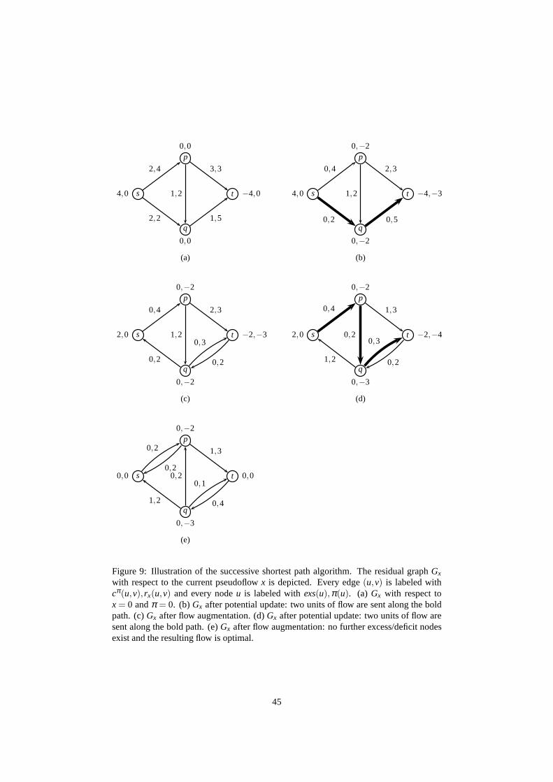
s4,0
p0,0
q
0,0
t −4,0
2,4
2,2
3,3
1,2
1,5
(a)
s4,0
p0,−2
q
0,−2
t −4,−3
(b)
0,4
0,2
2,3
1,2
0,5
s2,0
p0,−2
q
0,−2
t −2,−3
(c)
0,4
0,2
2,3
1,20,3
0,2
s2,0
p0,−2
q
0,−3
t −2,−4
(d)
0,4
1,2
1,3
0,20,3
0,2
s0,0
p0,−2
q
0,−3
t 0,0
(e)
0,2
0,2
1,2
1,3
0,20,1
0,4
Figure 9: Illustration of the successive shortest path algorithm. The residual graphGx
with respect to the current pseudoflowx is depicted. Every edge(u,v) is labeled withcπ(u,v), rx(u,v) and every nodeu is labeled withexs(u),π(u). (a) Gx with respect tox= 0 andπ = 0. (b)Gx after potential update: two units of flow are sent along the boldpath. (c)Gx after flow augmentation. (d)Gx after potential update: two units of flow aresent along the bold path. (e)Gx after flow augmentation: no further excess/deficit nodesexist and the resulting flow is optimal.
45

pseudoflow that we obtain fromx by sending∆ units alongP satisfies the reduced costoptimality conditions with respect toπ− δ .
It remains to be shown that the algorithm terminates. In eachiteration,∆ is chosen suchthat eithers or t become balanced or one of the edge onP becomes saturated. Eachiteration therefore strictly reduces the excess of the chosen source nodes. Since weassume that all input data is integral, the excess ofs is reduced by at least 1. The algorithmtherefore terminates after at mostnB iterations. Each iteration requires to solve a singlesource shortest path problem with respect tocπ . Because the reduced costscπ are non-negative, we can use Dijkstra’s algorithm which requiresO(m+nlogn) time. The overallrunning time of the successive shortest path algorithm is thusO(nB(m+nlogn)).
6.5 Primal-Dual Algorithm
We use linear programming duality to derive our third algorithm for the minimum costflow problem. We associate a dual variableπ(u) with every nodeu ∈ V andα(e) withevery edgee∈ E. The dual of the linear program (6) is as follows:
maximize ∑u∈V
b(u)π(u)−∑e∈E
w(e)α(e)
subject to π(u)−π(v)−α(u,v) ≤ c(u,v) ∀(u,v) ∈ Eα(e) ≥ 0 ∀e∈ E
(8)
As in the previous section, let the reduced cost of an edge(u,v) ∈ E be defined ascπ(u,v) = c(u,v)− π(u) + π(v). The above constraints then require that−α(u,v) ≤cπ(u,v) andα(u,v) ≥ 0 for every edge(u,v) ∈ E. Since the dual has a maximizationobjective and because capacities are nonnegative, an optimal solution to (8) satisfiesα(u,v) = max0,−cπ(u,v). In a sense, the dual variableα(u,v) are therefore redun-dant: Given optimal dual valuesπ(u) for everyu ∈ V, we can extend this solution to afeasible dual solution(π ,α) of (8) using the above relation.
We next derive thecomplementary slackness conditionsof the primal linear program (6)and the dual linear program (8):
1. Primal complementary slackness condition:for every edgee∈ E:
f (e)> 0 ⇒ α(e) =−cπ(e),
which is equivalent to
f (e) > 0 ⇒ cπ(e)≤ 0.
2. Dual complementary slackness condition:for every edgee∈ E:
α(e)> 0 ⇒ f (e) = w(e),
46

which is equivalent to
cπ(e)< 0 ⇒ f (e) = w(e).
Theorem 6.6(Complementary slackness optimality conditions). A feasible flow f of G isa minimum cost flow if and only if there exist dual valuesπ(u) for every u∈V satisfyingthat for every edge e∈ E:
1. If cπ(e)> 0 then f(e) = 0.2. If cπ(e)< 0 then f(e) = w(e).
Proof. The proof follows directly from the complementary slackness conditions.
The complementary slackness optimality conditions can actually be seen to be equivalentto the reduced cost optimality conditions that we introduced earlier:
Theorem 6.7. A feasible flow f satisfies the reduced cost optimality conditions with re-spect to node potentialsπ : V→ R if and only if f satisfies the complementary slacknessoptimality conditions with respect toπ .
Proof. Supposecπ(u,v)≥ 0 for every(u,v) ∈ Ef . Let (u,v) ∈ E and supposecπ(u,v)<0. Then(u,v) /∈ Ef and thusf (u,v) = w(u,v). Next supposecπ(u,v) > 0. Becausecπ(v,u) =−cπ(u,v)< 0, the backward edge(v,u) is not part ofGf and thusf (u,v) = 0.
Assume that the complementary slackness conditions are satisfied for every edge(u,v) ∈E. Consider a forward edge(u,v) ∈ Ef . Then f (u,v) < w(u,v) and thuscπ(u,v) ≥ 0.Next consider a backward edge(v,u) ∈ Ef . Then f (u,v)> 0 and thuscπ(u,v)≤ 0. Sincecπ(v,u) =−cπ(u,v), we conclude thatcπ(v,u)≥ 0.
The primal-dual algorithm for the minimum cost flow problem follows a generalprimal-dual paradigm: We start with an infeasible primal solutionx and a feasible dual solutionπ . We ensure that the algorithm satisfies the complementary slackness conditions withrespect tox andπ throughout the entire execution of the algorithm. The algorithm suc-cessively reduces the degree of infeasibility of the primalsolutionx with respect to thecurrent dual solutionπ . If no further improvement is possible, thenπ will be updated soas to ensure that the infeasibility ofx can be further reduced. The dual solutionπ remainsfeasible throughout the entire process. Eventually,x is a feasible primal solution and thusa minimum cost flow.
The algorithm works with a transformed instance of the problem having exactly one ex-cess and one deficit node: Augment the original graph by adding a super-sources anda super-target. Add an edge(s,u) for every nodeu ∈ V with b(u) > 0 of capacityw(s,u) = b(u) and costc(s,u) = 0. Similarly, add an edge(u, t) for every nodeu∈V withb(u) < 0 of capacityw(u, t) = −b(u) and costc(u, t) = 0. Let b(s) = ∑u∈V:b(u)>0b(u)andb(t) = ∑u∈V:b(u)<0b(u). All other balances are set to zero. Clearly, every minimumcost flow in the augmented network corresponds to a minimum cost flow in the originalnetwork and vice versa. Subsequently, we will use the augmented network.
47

The algorithm starts with the pseudoflowx(e) = 0 for everye∈ E and dualπ(u) = 0for everyu ∈ V. Note thatx is an infeasible primal solution andπ is a feasible dualsolution. Alsox andπ satisfy the complementary slackness conditions because for everyedgee∈ E, x(e) = 0 andcπ(e) = c(e)≥ 0.
In order to reduce the infeasibility ofx, the algorithm basically pushes as much flow aspossible froms to t along shortests, t-paths inGx. Let δ : V → R be the shortest pathdistances froms to all other nodesu ∈ V in Gx with respect tocπ . Defineπ ′ = π − δ .Then every shortests, t-path inGx with respect tocπ is a zero cost path with respect tocπ ′
and vice versa. Let theadmissible graph G0x be the subgraph ofGx = (V,Ex) that consistsof all edgese∈ Ex with cπ ′(e) = 0. The algorithm computes a maximum flowg0 in G0
x,where the capacities of the edges are their respective residual capacities. We can thenaugmentx by g0 in the obvious way: Increase the flow valuex(u,v) of every forward edge(u,v) ∈ E by g0(u,v) and decrease the flow valuex(u,v) of every backward edge(v,u)by g0(v,u). As a result, the excess ats is reduced by the flow value|g0|. It is not hardto see that the resulting flowx′ is a pseudoflow. Moreover, in light of Theorem6.7 andCorollary6.1, x′ satisfies the complementary slackness conditions with respect to the newfeasible dualπ ′.
The algorithm continues in this manner until eventually thetotal excess ofs is exhaustedand the pseudoflowx becomes a flow. Since the algorithm maintains the invariant thatxandπ satisfy the complementary slackness conditions andπ is a feasible dual solution,x(and alsoπ) are eventually optimal solutions to the respective linearprograms in (6) (and(8)).
The algorithm is summarized in Algorithm11; see Figure10 for an illustration.
Input : directed graphG= (V,E), capacity functionw : E→ R+, cost functionc : E→ R+ and balance functionb : V→R.
Output : minimum cost flowx : E→R+.
1 Initialize: x(u,v) = 0 for every(u,v) ∈ E andπ(u) = 0 for everyu∈V2 exs(s) = b(s)3 while exs(s)> 0 do4 compute shortest path distancesδ : V→ R from s to all other nodesu∈V in
Gx with respect tocπ
5 updateπ ← π− δ6 construct the admissible networkG0
x
7 compute a maximum flowg0 from s to t in G0x
8 augmentx by g0
9 updatex, exs(s), Gx andcπ
10 end11 return x
Algorithm 11: Primal-dual algorithm.
Theorem 6.8. The primal-dual algorithm computes a minimum cost flow in timeO(minnC,nB ·nm2).
48

s
4,0
p0,0
q0,0
x
0,0
y
0,0
t
−4,0
0,2
0,2
1,1
2,1
2,1
1,1
0,2
0,2
(a)
s
4,0
p0,0
q0,−1
x
0,0
y
0,−2
t
−4,−1
0,2
0,2
0,1
0,1
0,1
0,1
0,2
1,2
(b)
s
2,0
p0,0
q0,−1
x
0,0
y
0,−2
t
−2,−1
0,1
0,1
0,1
0,1
0,0
0,1
0,1
0,1
0,2
1,2
(c)
s
2,0
p0,0
q0,−2
x
0,0
y
0,−2
t
−2,−2
0,1
0,1
0,1
0,1
0,0
0,1
0,1
0,1
0,2
0,2
(d)
s
0,0
p0,0
q0,−2
x
0,0
y
0,−2
t
0,−2
0,2
0,2
0,0
0,1
0,1
0,1
0,2
0,2
(e)
Figure 10: Illustration of the primal-dual algorithm. The residual graphGx with respectto the current pseudoflowx is depicted. Every edge(u,v) is labeled withcπ(u,v), rx(u,v)and every nodeu is labeled withexs(u),π(u). (a) Gx with respect tox = 0 andπ = 0of the transformed network of the example instance depictedin Figure8(a). (b)Gx afterpotential update: max flow inG0
x has value 2. (c)Gx after flow augmentation. (d)Gx afterpotential update: max flow inG0
x has value 2. (e)Gx after flow augmentation: excess ofsource nodes is zero and the resulting flow is optimal.
49

Proof. The correctness of the algorithm follows from the discussion above.
Observe that in each iteration, the excess ofs is reduced by at least 1 (assuming integercapacities and balances). The maximum number of iterationsis thus at mostnB, which isthe maximum excess ofsat the beginning of the algorithm.
We can establish a second bound on the number of iterations: In each iteration,g0 is amaximum flow inG0
x. By the max-flow min-cut theorem, there is a cut(X, X) in G0x such
that for every edge(u,v) with u ∈ X andv ∈ X, g0(u,v) = rx(u,v). As a consequence,after the augmentation, all these edges vanish from the residual graphGx′ of the new flowx′. Thus, everys, t-path inGx′ has length at least 1 with respect tocπ ′(u,v) (because edgecosts are integral). The potential oft therefore reduces by at least 1 in the next iteration.Note that no node potentialπ(u) for u 6= s can ever be less than−nC (think about it!).The total number of iterations is therefore bounded bynC.
The running time of each iteration is dominated by the shortest path and max flow com-putations. The total running time is thus at mostO(minnC,nB ·nm2).
References
The presentation of the material in this section is based on [1, Chapter 9].
50
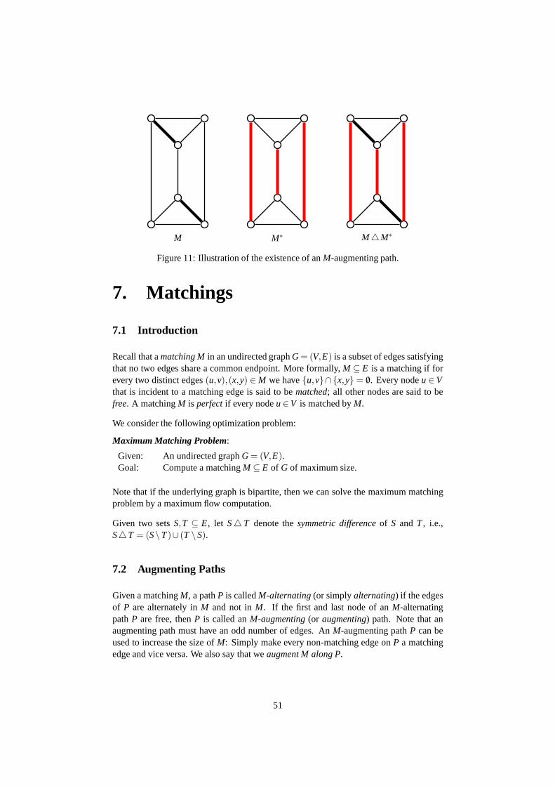
M M∗ MM∗
Figure 11: Illustration of the existence of anM-augmenting path.
7. Matchings
7.1 Introduction
Recall that amatching Min an undirected graphG= (V,E) is a subset of edges satisfyingthat no two edges share a common endpoint. More formally,M ⊆ E is a matching if forevery two distinct edges(u,v),(x,y) ∈M we haveu,v∩x,y = /0. Every nodeu∈Vthat is incident to a matching edge is said to bematched; all other nodes are said to befree. A matchingM is perfectif every nodeu∈V is matched byM.
We consider the following optimization problem:
Maximum Matching Problem:
Given: An undirected graphG= (V,E).Goal: Compute a matchingM ⊆ E of G of maximum size.
Note that if the underlying graph is bipartite, then we can solve the maximum matchingproblem by a maximum flow computation.
Given two setsS,T ⊆ E, let S T denote thesymmetric differenceof S and T, i.e.,ST = (S\T)∪ (T \S).
7.2 Augmenting Paths
Given a matchingM, a pathP is calledM-alternating(or simplyalternating) if the edgesof P are alternately inM and not inM. If the first and last node of anM-alternatingpathP are free, thenP is called anM-augmenting(or augmenting) path. Note that anaugmenting path must have an odd number of edges. AnM-augmenting pathP can beused to increase the size ofM: Simply make every non-matching edge onP a matchingedge and vice versa. We also say that weaugment M along P.
51

r
u v
Figure 12: Illustration of an alternating tree. The nodes inX andY are indicated in whiteand gray, respectively. Note that there is an augmenting path from r to v.
Theorem 7.1. A matching M in a graph G= (V,E) is maximum if and only if there is noM-augmenting path.
Proof. SupposeM is maximum and there is anM-augmenting pathP. Then augmentingM alongP gives a new matchingM′ = MP of size|M|+1, which is a contradiction.
Suppose thatM is not maximum. LetM∗ be a maximum matching. Consider the symmet-ric differenceMM∗. BecauseM andM∗ are matchings, the subgraphG′= (V,MM∗)consists of isolated nodes and node-disjoint paths and cycles. The edges of every suchpath or cycle belong alternately toM andM∗. Each cycle therefore has an even numberof edges. Because|M∗|> |M| there must exist one pathP that has more edges ofM∗ thanof M. P is anM-augmenting path; see Figure11for an illustration.
7.3 Bipartite Graphs
The above theorem gives an idea how to compute a maximum matching: Start with theempty matchingM = /0. Find anM-augmenting pathP and augmentM alongP. Repeatthis procedure until noM-augmenting path exists andM is maximum.
A natural approach to search for augmenting paths is to iteratively build analternatingtree. SupposeM is a matching andr is a free node. We inductively construct a treeTrooted atr as follows. We partition the node set ofT into two setsX andY: For everynodeu∈X, there is an even-length alternating path fromr to u in T; for every nodeu∈Y,there is an odd-length alternating path fromr to u in T. We start withX = r andY = /0and then iteratively extendT using the following operation:
EXTEND TREE USING(u,v):(Precondition:(u,v) ∈ E, u∈ X, v /∈ X∪Y and(v,w) ∈M)Add edge(u,v) to T, v to Y, edge(v,w) to T andw to X
This way we obtain a layered tree rooted atr (starting with layer 0); see Figure12 foran illustration. All nodes inX are on even layers and all nodes inY are on odd layers.Moreover, every node in layer 2i−1 (i ≥ 1) is matched to a node in layer 2i. In particular,|X|= |Y|+1.
52

Input : undirected bipartite graphG= (V,E).Output : maximum matchingM.
1 Initialize: M = /02 foreach r ∈V do3 if r is matchedthen continue4 else5 X = r, Y = /0, T = /06 while there exists an edge(u,v) ∈ E with u∈ X and v/∈ X∪Y do7 if v is freethen AUGMENT MATCHING USING (u,v)8 elseEXTEND TREE USING(u,v)9 end
10 end11 end12 return M
Algorithm 12: Augmenting path algorithm.
Suppose that during the extension of the alternating treeT we encounter an edge(u,v)∈Ewith u∈X andv /∈ X∪Y being a free node. We have then found an augmenting path fromr to v; see Figure12.
AUGMENT MATCHING USING (u,v)(Precondition:(u,v) ∈ E, u∈ X, v /∈ X∪Y free)AugmentM along the concatenation of ther,u-path inT with edge(u,v)
These two operations form the basis of the augmeting path algorithm given in Algo-rithm 12.
The correctness of the algorithm depends on whether alternating trees truly capture allaugmenting paths. Clearly, whenever the algorithm finds an augmenting path starting atr, this is an augmenting path. But can we conclude that there isno augmenting path ifthe algorithm does not find one? As it turns out, the algorithmworks correctly if theunderlying graph satisfies theunique label property: A graph satisfies theunique labelpropertywith respect to a given matchingM and a root noder if the above tree buildingprocedure uniquely assigns every nodeu∈V(T) to one of the setsX andY, irrespectiveof the order in which the nodes are examined.
Lemma 7.1. Suppose a graph satisfies the unique label property. If thereexists an M-augmenting path, then the augmenting path algorithm finds it.
Proof. Let P = 〈r, . . . ,u,v〉 be an augmenting path with respect toM. Because of theunique label property, the algorithm always ends up with adding nodeu to X and thusdiscovers an augmenting path via edge(u,v).
Using the above characterization, we can show that the augmenting path algorithm givenin Algorithm 12 is correct for bipartite graphs: Recall that in a bipartite graph, the nodesetV is partitioned into two setsV0 andV1. Every node that is part ofV(T) and belongs
53

r x b
p u
q v
z
(a)
r x b
z
(b)
Figure 13: Illustration of a blossom shrinking. (a) The odd cycle B = 〈b, p,u,v,q,b〉constitutes a blossom with baseb and stem〈r,x,b〉. Note that there is an augmentingpath fromz to r via edge(u,v). (b) The resulting graph after shrinking blossomB into asuper-nodeb.
to the setVi with r ∈ Vi is added toX; those that belong toV1−i are added toY. Thusbipartite graphs satisfy the unique label property.
Theorem 7.2. The augmenting path algorithm computes a maximum matching in bipar-tite graphs in time O(nm).
Proof. The correctness of the algorithm follows from the discussion above. Note that eachiteration can be implemented to run in timeO(n+m) and there are at mostn iterations.
7.4 General Graphs
It is not hard to see that graphs do in general not satisfy the unique label property. Consideran odd cycle consisting of three edges(r,u),(u,v),(v, r) and suppose that(u,v) ∈M andr is free. Then the algorithm addsu to Y if it considers edge(r,u) first, while it addsuto X if it considers edge(r,v) first. Odd cycles are precisely the objects that cause thisdilemma (and which are not present in bipartite graphs).
A deep insight that was first gained by Edmonds in 1965 is that one can “shrink” such oddcycles. Suppose during the construction of the alternatingtree, the algorithm encountersan edge(u,v) with u,v∈ X; see Figure13(a). Letb be the lowest common ancestor ofu andv in T. Note thatb∈ X. Consider the cycleB that follows the uniqueb,u-path inT, then edge(u,v) and then the uniquev,b-path inT. B is an odd length cycle, whichis also called ablossom. The nodeb is called thebaseof B. The even length path fromb to the root noder is called thestemof B; if r = b then we say that the stem ofB isempty. Suppose we shrink the cycleB to a super-node, which we identify withb; seeFigure13(b). Note that the super-nodeb belongs toX after shrinking.
SHRINK BLOSSOM USING(u,v):(Precondition:(u,v) ∈ E andu,v∈ X)Let b be the lowest common ancestor ofu andv in T.Shrink the blossomB= 〈b, . . . ,u,v, . . . ,b〉 to a super-nodeb.
54

Let G′ be the resulting graph and letM′ be the restriction ofM to the edges ofG′. Thenext two lemmas show that by shrinking blossoms, we do not addor lose any augmentingpaths.
Lemma 7.2. Suppose there is an M′-augmenting path P′ from r to v (or the respectivesuper-node) in G′. Then there is an M-augmenting path from r to v in G.
Proof. If P′ does not involve the super-nodeb, thenP′ is also an augmenting path inG.SupposeP′ contains the super-nodeb. There are two cases we need to consider:
Case 1:r 6= b. Let P′ = 〈r, . . . ,x,b,z, . . . ,v〉 be the augmenting path inG′. Let P′rx andP′zvrefer to the subpaths〈r, . . . ,x〉 and〈z, . . . ,v〉 of P′, respectively. Note that(x,b) ∈M′ and(b,z) /∈M′. If we expand the blossomB corresponding to super-nodeb, thenb is the baseof B with incident matching edge(x,b). Let p be the node ofB such that(p,z) is part ofG. Then there is an even lengthM-alternating pathPbp= 〈b, . . . , p〉 from b to p in B. ThepathP= 〈P′rx,(x,b),Pbp,(p,z),P′zv〉 is anM-augmenting path inG.
Case 2:r = b. Let P′ = 〈b,z, . . . ,v〉 be the augmenting path inG′. Let P′zv refer to thesubpath〈z, . . . ,v〉 of P′. If we expand the blossomB corresponding to super-nodeb, thenb is the base ofB which is free. Letp be the node ofB such that(p,z) is part ofG. Thenthere is an even lengthM-alternating pathPbp = 〈b, . . . , p〉 from b to p in B. The pathP= 〈b,Pbp,(p,z),P′zv〉 is anM-augmenting path inG.
Lemma 7.3. Suppose there is an M-augmenting path P from r to v in G. Then there is anM′-augmenting path from r to v (or the respective super-nodes)in G′.
Proof. We assume without loss of generality thatr andv are the only free nodes withrespect toM. (Otherwise, we can remove all other free nodes fromG without affectingP.) If P has no nodes in common with the nodes of the blossomB, thenP is an M′-augmenting path inG′ and we are done. SupposeP= 〈r, . . . ,v〉 contains some nodes ofB. We consider two cases:
Case 1: The stem ofB is empty. The baseb of B is then a free node and therefore coincideswith one of the endpoints ofP. Assume thatr = b; the other case follows similarly. Letpbe the last node ofP that is part ofB and letPpv= 〈p,z, . . . ,v〉 be the subpath ofP startingat p. Note that(p,z) /∈M. The pathP′ = 〈b,z, . . . ,v〉 is then anM′-augmenting path inG′.
Case 2: The stem ofB is non-empty. LetPrb = 〈r, . . . ,b〉 be the stem ofB. Consider thematchingM = MPrb. Thenr is matched inM and thusb andv are the only free nodeswith respect toM. Further,|M|= |M|. Note thatM is not a maximum matching (becausethere is anM-augmenting path inG) and thus alsoM is not a maximum matching. Thus,there is anM-augmenting pathP in G that starts atb and ends atv. Note that the stemof B with respect toP is empty and we can thus use the proof of Case 1 to show that thecontracted graphG′ contains anM′-augmenting path fromb to v. Note thatM′ is differentfrom M′. However, because|M′|= |M′| we conclude thatG′ must contain an augmentingpath with respect toM′ as well.
55

The matching algorithm for general graphs is also known as the blossom-shrinkingalgo-rithm. The algorithm maintains a graphG′ of super-nodes and a respective matchingM′
on the super-nodes throughout each iteration. At the end of each iteration, all super-nodesof G′ are expanded and the matchingM on the original graph is obtained fromM′ asdescribed in the proof of Lemma7.2.
Input : undirected graphG= (V,E).Output : maximum matchingM.
1 Initialize: M = /02 foreach r ∈V do3 if r is matchedthen continue4 else5 G′←G andM′←M.6 X←r, Y← /0, T ← /07 while there exists an edge(u,v) ∈ E′ with u∈ X and v/∈Y do8 if v is free, v6= r then AUGMENT MATCHING USING (u,v)9 else ifv /∈ X∪Y, (v,w) ∈M′ then EXTEND TREE USING(u,v)
10 elseSHRINK BLOSSOM USING(u,v)11 end12 ExtendM′ to a matchingM of G by expanding all super-nodes ofG′.13 end14 end15 return M
Algorithm 13: Blossom shrinking algorithm.
Theorem 7.3. The blossom-shrinking algorithm computes a maximum matching in gen-eral graphs in time O(nmα(n, m
n )).
Proof. The correctness of the algorithm follows from Lemmas7.2 and 7.3 and The-orem 7.1. It remains to show that the algorithm can be implemented to run in timeO(mα(n, m
n )) per iteration. The key here is to maintain an implicit representation ofthe graphG′ of super-nodes: We keep track of the partition of the original nodes intosuper-nodes by means of aunion-finddata structure. Considering an edge(u,v) ∈ E dur-ing an iteration, we need to check whether edge(u,v) is part ofG′. This can be done byverifying whetheru andv belong to the same set of the partition. Shrinking a blossom istantamount to uniting the node sets of the respective super-nodes. We have at most 2mfindandn union operations per iterations and these operations take timeO(n+mα(n, m
n )). Allremaining operations (extending the tree, augmenting the matching, extracting the match-ing onG) can be done in timeO(n+m) per iteration. The time bound follows.
There are algorithms with better running times for the matching problem. For the bipartitecase, Hopcroft and Karp showed that the running time of the augmenting path algorithmcan be reduced toO(
√nm). The basic idea is to augment the current matching in each
iteration by a maximal set of node-disjoint shortest paths (in terms of number of edges).Using this idea, one can show that the shortest path lengths increase with each iteration.
56
Now, fix an arbitrary matchingM and suppose|M| ≤ k−√
k, wherek = |M∗| is the car-dinality of a maximum matching. It is not hard to see that thenthere is anM-augmentingpath of length at most 2
√k+1. That is, after at most 2
√k+1 iterations, the algorithm
has found a matchingM of size at leastk−√
k. After at most√
k additional iterations,the algorithm terminates with a maximum matching. Each iteration can be implementedto run in timeO(n+m), which gives a total running timeO(
√km) = O(
√nm). A similar
idea can be used in the general case to obtain an algorithm that computes a maximummatching in timeO(
√nm).
References
The presentation of the material in this section is based on [1, Chapter 12] and [2, Chapter5].
57

b
b
b
b
b
bb
b bb
b bb
bb
b
S
(a)
b
b
b
b
b
bb
b bb
b bb
bb
b
b v
wTx≤ t
conv-hull(S)
(b)
Figure 14: (a) Finite point setS. (b) Convex hullconv-hull(S) and a separating inequalityfor v /∈ conv-hull(S).
8. Integrality of Polyhedra
8.1 Introduction
Many algorithms for combinatorial optimization problems crucially exploit min-max re-lations in order to prove optimality of the computed solution. We have seen examplesof such algorithms for the maximum flow problem, minimum costflow problem and thematching problem. A question that arises is whether there isa general approach to derivesuch min-max relations. As we will see in this section, such relations can often be derivedvia polyhedral methods.
8.2 Convex Hulls
Suppose we are given a finite setS= s1, . . . ,sk⊆Rn of n-dimensional vectors. A vectorx ∈ Rn is a convex combinationof the vectors inS if there exist non-negative scalarsλ1, . . . ,λk with ∑k
i=1 λi = 1 such thatx= ∑ki=1 λisi . Theconvex hullof S is defined as the
set of all convex combinations of vectors inS. Subsequently, we useconv-hull(S) to referto the convex hull ofS.
Suppose we want to solve the following mathematical programming problem: Givensomew ∈ Rn, maxwTx | x ∈ S. Intuitively, it is clear that this is the same as maxi-mizingwTx over the convex hull ofS.
Theorem 8.1. Let S⊆Rn be a finite set and let w∈ Rn. Then
maxwTx | x∈ S= maxwTx | x∈ conv-hull(S).
58

Proof. Let x∈ conv-hull(S). Then
wTx= λ1wTs1+ · · ·+λkwTsk ≤maxwTx | x∈ S.
Thus maxwTx | x∈ conv-hull(S) ≤maxwTx | x∈ S. Equality now follows becauseS⊆ conv-hull(S).
The next proposition states that ifv∈Rn\conv-hull(S) then there must exist aseparatinginequality wTx≤ t that separatesv from conv-hull(S), i.e.,wTx≤ t for all x∈ conv-hull(S)butwTv> t.
Theorem 8.2. Let S⊆ Rn be a finite set and let v∈ Rn \ conv-hull(S). Then there is aseparating inequality wTx≤ t that separates v from conv-hull(S).
Proof. Note that verifying whetherv ∈ conv-hull(S) is equivalent to checking whetherthere is a solution(λ1, . . . ,λk) to the following linear system:
k
∑i=1
λisi = v (9)
k
∑i=1
λi = 1 (10)
λi ≥ 0 ∀i ∈ 1, . . . ,k (11)
Conversely,v ∈ Rn \ conv-hull(S) iff the above linear system has no solution. UsingFarkas Lemma (see below) with
A=
s1,1 . . . sk,1... . . .
...s1,n . . . sk,n
1 . . . 1
, x=
λ1...
λk
and b=
v1...
vn
1
we obtain thatv∈ Rn \ conv-hull(S) iff there exists ay∈ Rn andz∈ R such that
(yT z)A≥ 0 and (yT z)b< 0,
or, equivalently,
yTsi ≥−z ∀i ∈ 1, . . . ,kyTv<−z.
By settingw=−y andt = z, we obtain thatwTsi ≤ t for everyi ∈ 1, . . . ,k. Theorem8.1implies thatwTx≤ t for everyx∈ conv-hull(S). Moreover,wTv> t, which concludes theproof.
We state the following proposition without proof.
59

(a)
b
bb
b
b
(b)
Figure 15: (a) Polytope described by five linear inequalities. (b) Faces of the polytope(indicated in bold).
Proposition 8.1(Farkas Lemma). The system Ax= b has a non-negative solution x≥ 0if and only if there is no vector y such that yTA≥ 0 and yTb< 0.
8.3 Polytopes
A polyhedron P⊆ Rn is described by a system of linear inequalities, i.e.,P = x ∈Rn | Ax≤ b. A polyhedronP is a polytopeif P is bounded, i.e., there existl ,u ∈ Rn
such thatl ≤ x≤ u for everyx∈ P.
An inequalitywTx≤ t is calledvalid for a polyhedronP if P⊆ x∈ Rn | wTx≤ t. Ahyperplaneis given byx∈Rn | wTx= t. It is called asupporting hyperplaneif wTx≤ tis valid for P andP∩x | wTx = t 6= /0. The intersection of a supporting hyperplanewith P is called aface. In the plane, the faces of a polyhedron are the edges and cornerpoints ofP.
Lemma 8.1. A non-empty set F⊆ P= x | Ax≤ b is a face of P if and only if for somesubsystem Ax≤ b of Ax≤ b, we have F= x∈ P | Ax = b. Moreover, if F is an(inclusionwise) minimal face of P, then the rank of A is equal to the rank of A.
A vectorv∈ P is avertexof P if v is a face ofP. A polyhedronP is pointedif it has atleast one vertex.
Lemma 8.2. If a polyhedron P is pointed then every minimal non-empty face of P is avertex.
Lemma 8.3. Let P= x | Ax≤ b and v∈ P. Then v is a vertex of P if and only if vcannot be written as a convex combination of vectors in P\ v.
Proof. Supposev is a vertex ofP and letAx≤ b be a subsystem ofAx≤ b such thatv = x∈ P | Ax = b. Supposev can be written as a convex combinationλ1x1+
60

· · ·+λkxk of vectorsx1, . . . ,xk ∈ P. ThenAxi = b for everyi ∈ 1, . . . ,k. But this is acontradiction to the assumption thatv is the unique solution to the systemAx= b.
Conversely, supposev cannot be written as a convex combination of vectors inP\ v.Let Ax≤ b consist of the inequalities ofAx≤ b which v satisfies with equality. LetF = x | Ax= b. It suffices to show thatF = v. Suppose that this is not true. Letu∈ F \v and consider the lineL= v+λ (u−v) | λ ∈R throughu andv. Clearly,L⊆F . For every inequalityaix≤ bi of Ax≤ b which is not part ofAx≤ b, we haveaix< bi .We can therefore determine a sufficiently smallε > 0 such thatv+ = v+ε(u−v)∈ P andv− = v− ε(u− v)∈ P. But v= 1
2(v++ v−), which is a contradiction.
Theorem 8.3. A polytope is equal to the convex hull of its vertices.
Proof. Let P be a polytope. SinceP is bounded,P must be pointed. LetV = v1, . . . ,vkbe the vertices ofP. Clearly, conv-hull(V) ⊆ P. It remains to be shown thatP ⊆conv-hull(V). Suppose there exists someu ∈ P\ conv-hull(V). Then by Theorem8.2,there exists an inequalitywTx≤ t that separatesu from conv-hull(V), i.e., wTx≤ t foreveryx∈ conv-hull(V) andwTu> t. Let t∗ = maxwTx | x∈ P and consider the faceF = x∈ P | wTx= t∗. Becauseu∈ P, we havet∗ ≥ wTu> t. That is,F contains novertex ofP, which is a contradiction.
Theorem 8.4. A set P is a polytope if and only if there exists a finite set V such that P isthe convex hull of V .
The above theorem suggests the following approach to obtaina min-max relation for acombinatorial optimization problem.
1. Formulate the combinatorial problemΠ as an optimization problem over a finitesetSof feasible solutions (e.g., by considering all characteristic vectors).
2. Determine a linear description ofconv-hull(S).3. Use duality of linear programming theory to obtain a min-max relation.
Note that by Theorem8.1, solving the problemΠ over S is equivalent to solving theproblem overconv-hull(S). By Theorem8.4, there must exist a polyhedral description ofconv-hull(S). Thus,Π can be described as a linear program. Dualizing and using strongduality, we can deduce a min-max relation for the problem.
We remark that the results given above show that the above approach as such is applicable.However, there are (at least) two difficulties here: (i) It isnot clear how to derive a lineardescription ofconv-hull(S) above. (ii) Even though such a description is guaranteed toexist, the number of linear inequalities might be by far larger than the size of the originalproblem. That is, even if we are able to come up with such a description, this might notlead to a polynomial-time algorithm.
We exemplify the above approach for theperfect matching problemin bipartite graphs.Let G= (V,E) be a bipartite graph. Recall that a matching isperfectif every node of thegraph is matched. DefinePM(G) ⊆ RE as the set of characteristic vectors of the perfectmatchings ofG.
Theorem 8.5(Birkhoff’s Theorem). Let G= (V,E) be a bipartite graph. The convex hull
61

of PM(G) is defined as
∑e=(u,v)∈E
xe = 1 ∀u∈V
xe ≥ 0 ∀e∈ E(12)
Proof. Let P be the polytope defined by (12). Clearly, each perfect matchingx∈ PM(G)
is contained inP. It suffices to show that all vertices ofP are integral. Suppose for the sakeof contradiction thatx is a vertex ofP that is not integral. LetE = e∈ E | 0< xe < 1be the fractional edges ofx. Because∑e=(u,v)∈E xe = 1 for every nodeu∈V, each nodeincident to an edge inE is incident to at least two edges inE. Thus, there exists a cycleC in E. Also,C must be even becauseG is bipartite. Letd ∈ RE be a vector that is 0 forall edges not inC and alternately 1 and−1 for the edges alongC. Because all edges ofC are contained inE, there is anε > 0 such thatx+ = x+ εd andx− = x− εd are inP.Note thatx= 1
2(x++ x−). But this is a contradiction to the assumption thatx is a vertex
of P.
8.4 Integral Polytopes
Many combinatorial optimization problems can naturally beformulated as an integer lin-ear program. Such programs are in general hard to solve. However, sometimes we areable to derive a polyhedral description of the problem: Suppose that by relaxing the in-tegrality constraints of the IP formulation of the optimization we obtain a linear programwhose feasible region is an integral polyhedron. We can thensolve the optimization prob-lem in polynomial time simply by computing an optimal solution to the LP, e.g., by usingKhachiyan’s ellipsoid method. An important question in this context is therefore whethera resulting polyhedron is integral. Proving integrality ofpolyhedra is often a difficult task.We next consider a technique that facilitates showing that apolyhedron is integral.
Subsequently, we concentrate on rational polyhedra, i.e.,polyhedra that are defined byrational linear inequalities. A rational polyhedronP is calledintegral if every non-emptyfaceF of P contains an integral vector. Clearly, it suffices to show that every minimalface ofP is integral because every face contains a minimal face. Notethat if P is pointedthen this is equivalent to showing that every vertex ofP is integral.
Lemma 8.4. Let B∈ Zm×m be an invertible matrix. Then B−1b is integral for everyintegral vector b if and only ifdet(B) =±1.
Proof. Suppose det(B) =±1. By Cramer’s Rule,B−1 is integral, which implies thatB−1bis integral for every integralb. Conversely, supposeB−1b is integral for every integralvectorb. Then alsoB−1ei is integral for alli ∈ 1, . . . ,m, whereei is theith unit vector.As a consequence,B−1 is integral. Thus, det(B) and det(B−1) are both integers. This incombination with det(B)det(B−1) = 1 implies that det(B) =±1.
A matrix A is totally unimodularif every square submatrix ofA has determinant 0, 1 or−1. Clearly, every entry in a totally unimodular matrix is 0, 1or−1.
62

Theorem 8.6. Let A∈ Zm×n be a totally unimodular matrix and let b∈ Zm. Then thepolyhedron P= x | Ax≤ b is integral.
Proof. Let F be a minimal face ofP. ThenF = x | Ax = b for some subsystemAx≤ b of Ax≤ b andA has full row rank. By reordering the columns ofA we maywrite A as(B N), whereB is a basis ofA. BecauseA is totally unimodular andB is abasis, det(B) = ±1. By Lemma8.4, it follows thatx = (B−1b
0 ) is an integral vector inF .
Let A∈ Rm×n be a matrix of full row rank. Abasis Bof A is a non-singular submatrix ofA of orderm. A matrix A of full row rank isunimodularif A is integral and each basisBof A has det(B) =±1.
Theorem 8.7. Let A∈ Zm×n be a matrix of full row rank. Then the polyhedron P=x | Ax= b, x≥ 0 is integral for every vector b∈ Zm if and only if A is unimodular.
Proof. SupposeA is unimodular. Letb∈Zm and letx be a vertex ofP. (Note that the non-negativity constraint ensures thatP has vertices.) Then there aren linearly independentconstraints satisfied byx with equality. The columns ofA corresponding to non-zeroentries ofx are linearly independent. We can extend these columns to a basis B of A.Note that det(B) = ±1 becauseA is unimodular. Thenx restricted to the coordinatescorresponding toB is B−1b, which is integral by Lemma8.4. The remaining entries ofxare zero. Thus,x is integral.
Assume thatP is integral for every integer vectorb. Let B be a basis ofA. We needto show that det(B) = ±1. By Lemma8.4, it suffices to show thatB−1v is integral forevery integral vectorv. Let v be an integral vector. Lety be an integral vector such thatz= y+B−1v≥ 0 and letb = Bz= B(y+B−1v) = By+ v. Note thatb is integral. Byadding zero components toz, we obtain a vectorz′ ∈ Zn such thatAz′ = Bz= b. Thenz′
is a vertex ofx | Ax= b, x≥ 0, becausez′ is in the polyhedron and satisfiesn linearlyindependent constraints with equality: them equationsAx= b and then−m equationsxi = 0 for the columnsi outside ofB. Soz′ is integral and thusB−1v= z−y is integral.
Theorem 8.8. Let A∈ Zm×n. The polyhedron P= x | Ax≤ b, x≥ 0 is integral forevery vector b∈ Zm if and only if A is totally unimodular.
Proof. It is not hard to show thatA is totally unimodular if and only if(A I) is unimodular,whereI is them×m identity matrix. By Theorem8.7, (A I) is unimodular if and onlyif P′ = z | (A I)z= b, z≥ 0 is integral for everyb ∈ Zm. The latter is equivalent toP= x | Ax≤ b, x≥ 0 being integral for everyb∈ Zm.
8.5 Example Applications
Theorem 8.9. A matrix A is totally unimodular if
1. each entry is0, 1 or −1;
63

2. each column contains at most two non-zeros;3. the set N of row indices of A can be partitioned into N1∪N2 so that in each column
j with two non-zeros we have∑i∈N1ai, j = ∑i∈N2
ai, j .
Proof. Suppose thatA is not totally unimodular. Lett be the smallest integer such thatBis a t× t square submatrix ofA with det(B) /∈ −1,0,1. SupposeB has a column witha single non-zero entry, saybk, j . By expanding the determinant along rowj (Laplaceexpansion), we obtain
det(B) =t
∑i=1
(−1)i+ jbi, jMi, j = (−1)k+ jbk, jMk, j
whereMi, j is theminordefined as the determinant of the submatrix obtained by removingrow i and columnj from B. By (1), bk, j ∈ −1,0,1 and because det(B) /∈ −1,0,1,Mk, j /∈ −1,0,1, which is a contradiction to the choice ofB. By (2), every column ofB must therefore contain exactly two non-zero entries. By (3), adding up the rows ofB(N1 with positive sign,N2 with negative sign) yields the zero vector. The row vectors aretherefore linearly dependent and thus det(B) = 0, which is a contradiction.
The incidence matrix A= (au,e) of an undirected graphG = (V,E) is ann×m matrix(n= |V| andm= |E|) such that for everyu∈V ande∈ E:
au,e =
1 if e= (u,v) ∈ E
0 otherwise.
The incidence matrix A= (au,e) of a directed graphG= (V,E) is ann×m matrix suchthat for everyu∈V ande∈ E:
au,e =
1 if e= (u,v) ∈ E
−1 if e= (v,u) ∈ E
0 otherwise.
The following corollary follows immediately from Theorem8.9.
Corollary 8.1. If A is an incidence matrix of an undirected bipartite graph or an inci-dence matrix of a directed graph, then A is totally unimodular.
Proof. The proof follows from Theorem8.9 by choosingN1 = V0 andN2 = V1 in thebipartite case (whereV =V0∪V1) andN1 =V andN2 = /0 in the directed case.
Recall that anode coverof an undirected graphG= (V,E) is a subsetC⊆V such that forevery edgee= (u,v) at least one of the endpoints is inC, i.e.,u,v∩C 6= /0. Letν(G) bethe size of a maximum matching ofG and letτ(G) be the size of a minimum node coverof G.
64

The size of a maximum matching can be formulated as an integerprogram:
ν(G) = maximize ∑e∈E
xe
subject to ∑e=(u,v)∈E
xe ≤ 1 ∀u∈V
xe ∈ 0,1 ∀e∈ E
Equivalently, we can write this IP in a more compact way:
ν(G) = 1Tx | Ax≤ 1, x≥ 0, x∈ Zm, (13)
whereA∈ Zn×m is the incidence matrix ofG with n= |V| andm= |E|.
Similarly, the size of a minimum node cover can be expressed as
τ(G) = minimize ∑u∈V
yu
subject to yu+ yv ≥ 1 ∀(u,v) ∈ Eyu ∈ 0,1 ∀u∈V
or, equivalently,
τ(G) = yT1 | ATy≥ 1, y≥ 0, y∈ Zn (14)
Theorem 8.10. Let G= (V,E) be a bipartite graph. The size of a maximum matching ofG is equal to the size of a minimum node cover of G, i.e.,ν(G) = τ(G).
Proof. Let A∈ Zn×m be the incidence matrix ofG with n= |V| andm= |E|. As observedabove, we can expressν(G) andτ(G) by the two integer linear programs (13) and (14).Consider the respective LP relaxations of (13) and (14):
ν ′(G) = 1Tx | Ax≤ 1, x≥ 0 (15)
τ ′(G) = yT1 | ATy≥ 1, y≥ 0 (16)
Note that both LPs are feasible. BecauseA is totally unimodular, both LPs have integraloptimal solutions and thusν(G) = ν ′(G) andτ(G) = τ ′(G). Finally, observe that (16) isthe dual of (15). By strong duality,ν ′(G) = τ ′(G), which proves the claim.
A matrix A is called aninterval matrixif every entry ofA is either 0 or 1 and the the 1’sof each row appear consecutively (without interfering zeros).
Theorem 8.11. Each interval matrix A is totally unimodular.
65

Proof. Let B be at× t submatrix ofA. Define at× t matrixN as follows:
N =
1 −1 0 . . . 0 00 1 −1 . . . 0 0...
......
. . ....
...0 0 0 . . . 1 −10 0 0 . . . 0 1
Note that det(N) = 1. ConsiderNBT . ThenNBT is a submatrix of an incident matrixof some directed graph. (Think about it!) Therefore,NBT is totally unimodular. Weconclude
det(B) = det(N)det(BT) = det(NBT) ∈ −1,0,1.
References
The presentation of the material in this section is based on [2, Chapter 6].
66

9. Complexity Theory
9.1 Introduction
The problems that we have considered in this course so far areall solvableefficiently.This means that we were always able to design an algorithm forthe respective optimiza-tion problem that solves every instance in time that is polynomially bounded in the sizeof the instance. For example, we have seen that every instance of theminimum spanningtree problemwith n vertices andm edges can be solved in timeO(m+nlogn). Unfortu-nately, for many natural and fundamental optimization problems efficient algorithms arenot known to exist. A well-known example of such a problem is the traveling salesmanproblem.
Traveling Salesman Problem (TSP):
Given: An undirected graphG= (V,E) and non-negative distancesd : E→Z+
on the edges.Goal: Find a tour that visits every vertex ofGexactly once (starting and ending
in the same vertex) and has minimum total length.
Despite 50 years of intensive research, no efficient algorithm has been found for the TSPproblem. On the other hand, researchers have also not been able to disprove the existenceof such algorithms. Roughly speaking, complexity theory aims to answer the questionif the research community has been too stupid or unlucky to find efficient algorithmsfor optimization problems such as the TSP problem, or that these problem are in factintrinsically more difficult than other problems. It provides a mathematical framework toseparate problems that are computationally hard to solve from the ones that are efficientlysolvable.
In complexity theory one usually considers decision problems instead of optimizationproblems.
Definition 9.1. A decision problemΠ is given by a set of instancesI. Each instanceI ∈ I specifies
• a setF of feasible solutions forI ;• a cost functionc : F → Z;• an integerK.
Given an instanceI = (F ,c,K) ∈ I, the goal is to decide whether there exists a feasiblesolutionS∈ F whose costc(S) is at mostK. If there is such a solution, we say thatI is a“yes-instance”; otherwise,I is a “no-instance”.
Example 9.1. The decision problem of the TSP problem is to determine whether for agiven instanceI = (G,d,K) ∈ I there exists a tour inG of total length at mostK.
Many decision problems can naturally be described without the need of introducing a costfunctionc and a parameterK. Some examples are the following ones.
67

Prime:
Given: A natural numbern.Goal: Determine whethern is a prime.
Graph Connectedness:
Given: An undirected graphG= (V,E).Goal: Determine whetherG is connected.
Hamiltonian Cycle:
Given: An undirected graphG= (V,E).Goal: Determine whetherG has a Hamiltonian cycle.
Subsequently, we will mostly focus on decision problems. For notational convenience wewill use the same naming as for the respective optimization counterparts (e.g.,TSPwillrefer to the decision problem of TSP); no confusion should arise from this.
Recall that an algorithmALG for a problemΠ is said to beefficient if it solves everyinstanceI ∈ I of Π in time that is bounded by a polynomial function of the size ofI .It is not hard to see that the decision version of an optimization problem is easier thanthe optimization problem itself. But in most cases, an efficient algorithm for solvingthe decision version can also be turned into an efficient algorithm for the optimizationproblem (e.g., by using binary search on the possible optimal value).
9.2 Complexity ClassesP and NP
Intuitively, the complexity classesP andNP refer to decision problems that can besolvedefficiently and those for which yes-instances can beverifiedefficiently, respectively. If weinsisted on formal correctness here, we would define these classes in terms of a specificcomputer model calledTuring machines. However, this is beyond the scope of this courseand we therefore take the freedom to introduce these classesusing a more high-level (butessentially equivalent) point of view.
We define the complexity classP (which stands forpolynomial-time).
Definition 9.2. A decision problemΠ belongs to the complexity classP if there existsan algorithm that for every instanceI ∈ I determines in polynomial time whetherI is ayes-instance or a no-instance.
All problems that we have treated so far in this course belongto this class. But also thelin-ear programming problem (LP)belongs to this class, even though the simplex algorithmis not a polynomial-time algorithm for LP (the interested reader is referred to Section 8.6in [6]). The simplex algorithm works almost always very fast in practice for any LP ofwhatever size, but as mentioned before the running time of analgorithm is determined byits worst-case running time. For most pivoting rules devised for the simplex algorithm,there have been constructed instances on which the algorithm has to visit an exponentialnumber of basic feasible solutions in order to arrive at an optimal one. A polynomial-timealgorithm for LP is theellipsoid method(the interested reader is referred to Section 8.7 in
68

[6]). This algorithm is an example where the time bound is polynomial in the logarithmof the largest coefficient in the instance next to the number of variables and number ofrestrictions. One of the most interesting open research questions in Operations Researchis whether there exists an algorithm for LP whose running time is a polynomial in thenumber of variables and the number of restrictions only.
Next we define the complexity classNP. NP does not stand for “non-polynomial-time”as one might guess, but for “non-deterministic polynomial-time” because this class isformally defined in terms of non-deterministic Turing machines.
Given a yes-instanceI ∈ I of a decision problemΠ, we say thatS is a certificateforI if S∈ F andc(S) ≤ K. Note that every yes-instanceI must have a certificate. Thespecialty of a problem inNP is that yes-instances admit certificates that can be verifiedinpolynomial time.
Definition 9.3. A decision problemΠ belongs to the complexity classNP if every yes-instanceI ∈ I admits a certificate whose validity can be verified in polynomial time.
Note that the polynomial-time verifiability ofS implies that the size ofS must be poly-nomially bounded in|I | (because we need to look atS to verify its validity). That is, thedefinition above also states that yes-instances of problemsin NP haveshort, i.e., polyno-mially bounded, certificates.
We consider some examples:
Example 9.2. The Hamiltonian cycle problem is inNP: A certificate for a yes-instancecorresponds to a set of edgesS⊆ E. One can verify inO(n) time whetherSconstitutes acycle inG that visits all vertices exactly once.
Example 9.3. Consider the decision variant of the linear programming problem:
Linear Programming Problem (LP):
Given: A setF of feasible solutionsx= (x1, . . . ,xn) defined bym linear constraints
F =
(x1, . . . ,xn) ∈ Rn≥0 :
n
∑i=1
ai j xi ≥ b j for every j = 1, . . . ,m
together with an objective functionc(x) = ∑ni=1cixi and a parameterK.
Goal: Determine whether there exists a feasible solutionx ∈ F that satisfiesc(x)≤ K.
LP is in NP: A certificate for a yes-instance corresponds to a solutionx= (x1, . . . ,xn). WeneedO(n) time to verify each of themconstraints andO(n) time to compute the objectivefunction valuec(x). The total time needed to check whetherx∈ F andc(x) ≤ K is thusO(nm).
69

9.3 Polynomial-time Reductions andNP-completeness
After thinking for a little while, we conclude thatP⊆ NP. Several decades of intensiveresearch seem to suggest that there are problems inNP that are intrinsically more difficultthan the ones inP and thusP 6= NP: Despite the many research efforts, no polynomial-time algorithms have been found for problems inNP such asTSP, Hamiltonian cycle,Steiner tree, etc. On the other hand, all attempts to show that these problems are in factharder than the ones inP failed as well. The question whetherP 6= NP is one of thebiggest mysteries in mathematics to date and constitutes one of the seven millennium-prize problems; seehttp://www.claymath.org/millenniumfor more information.
Complexity theory attempts to give theoretical evidence tothe conjecture thatP 6= NP. Itdefines within the complexity classNPa subclass of most difficult problems, the so-calledNP-completeproblems. This subclass is defined in such a way that if foranyof theNP-complete problems there will ever be found a polynomial-time algorithm then this impliesthat foreveryproblem inNP there exists a polynomial-time algorithm, and thusP= NP.The definition of this class crucially relies on the notion ofpolynomial-time reductions:
Definition 9.4. A polynomial-time reductionfrom a decision problemΠ1 to a decisionproblemΠ2 is a functionϕ : I1→I2 that maps every instanceI1∈ I1 of Π1 to an instanceI2 = ϕ(I1) ∈ I2 of Π2 such that:
1. the mapping can be done in time that is polynomially bounded in the size ofI1;2. I1 is a yes-instance ofΠ1 if and only if I2 is a yes-instance ofΠ2.
If there exist such a polynomial-time reduction fromΠ1 to Π2 then we say thatΠ1 can bereduced toΠ2, and we will writeΠ1Π2.
Lets think about some consequences of the above definition interms of polynomial-timecomputability. SupposeΠ1Π2. ThenΠ2 is more difficult to solve thanΠ1 (which alsojustifies the use of the symbol). To see this, note that every polynomial-time algorithmALG2 for Π2 can be used to derive a polynomial-time algorithmALG1 for Π1 as follows:
1. Transform the instanceI1 of Π1 to a corresponding instanceI2 = ϕ(I1) of Π2.2. RunALG2 on I2 and report thatI1 is a yes-instance if and only ifALG2 concluded
thatI2 is a yes-instance.
By the first property of Definition9.4, the transformation in Step 1 above takes time poly-nomial in the sizen1 = |I1| of I1. As a consequence, the sizen2 = |I2| of I2 is polynomiallybounded inn1. (Think about it!) In Step 2,ALG2 solvesI2 in time polynomial in the sizen2 of I2, which is polynomial in the sizen1.3 The overall time needed byALG1 to outputa solution forI1 is thus bounded by a polynomial inn1. Note that the second property ofDefinition9.4ensures thatALG1 correctly identifies whetherI1 is a yes-instance or not.
Observe the existence of a polynomial-time algorithm forΠ1 has in general no implica-tions for the existence of a polynomial-time algorithm forΠ2, even if we assume that wecan compute the inverse ofϕ efficiently. The reason for that is thatϕ is not necessarily aone-to-one mapping and may thus map the instances ofΠ1 to a subset of the instances of
3Observe that we exploit here that ifp1, p2 are polynomial functions inn then p2(p1(n)) is a polynomialfunction inn.
70

Π2 which correspond to easy instances ofΠ2. Thus, being able to efficiently solve everyinstance ofΠ1 reveals nothing about the problem of solvingΠ2.
It is not hard to show that polynomial-time reductions are transitive:
Lemma 9.1. If Π1Π2 andΠ2Π3 thenΠ1Π3.
We can now define the class ofNP-completeproblems.
Definition 9.5. A decision problemΠ is NP-completeif
1. Π belongs toNP;2. every problem inNP is polynomial-time reducible toΠ.
Intuitively, the above definition states that anNP-complete problem is as difficult as anyother problem inNP. The above definition may not seem very helpful at first sight:Howdo we prove thateveryproblem inNP is polynomial-time reducible to the problemΠ weare interested in? Lets assume for the time being that there are some problems that areknown to beNP-complete. In order to proveNP-completeness ofΠ it is then sufficient toshow thatΠ is in NP and thatsome NP-complete problem is polynomial-time reducibleto Π. (Think about it!) That is, showingNP-completeness of a problem becomes mucheasier now because we “just” need to find an appropriateNP-complete problem that canbe reduced to it. Nevertheless, we remark that the reductions of manyNP-completenessproofs are highly non-trivial and often require a deep understanding of the structural prop-erties of the problem.
The classNP has a very precise definition in terms of executions of non-deterministicTurning machines (which we skipped and persist in skipping), which enabled StevenCook in 1974 to prove that any such execution can be reduced toan instance of a fa-mous problem in Boolean logic called thesatisfiability problem (SAT)(stated below).Thus, Cook provided us with a problem that isNP-complete. Starting from this, manyother problems were proven to beNP-complete.
In a way, proving that a problem isNP-complete is a beautiful way of stating:4
“I can’t find an efficient algorithm, but neither can all thesefamous people.”
4The illustration is taken from the book [4], which is an excellent book on the complexity of algorithmscontaining many fundamentalNP-completeness proofs.
71
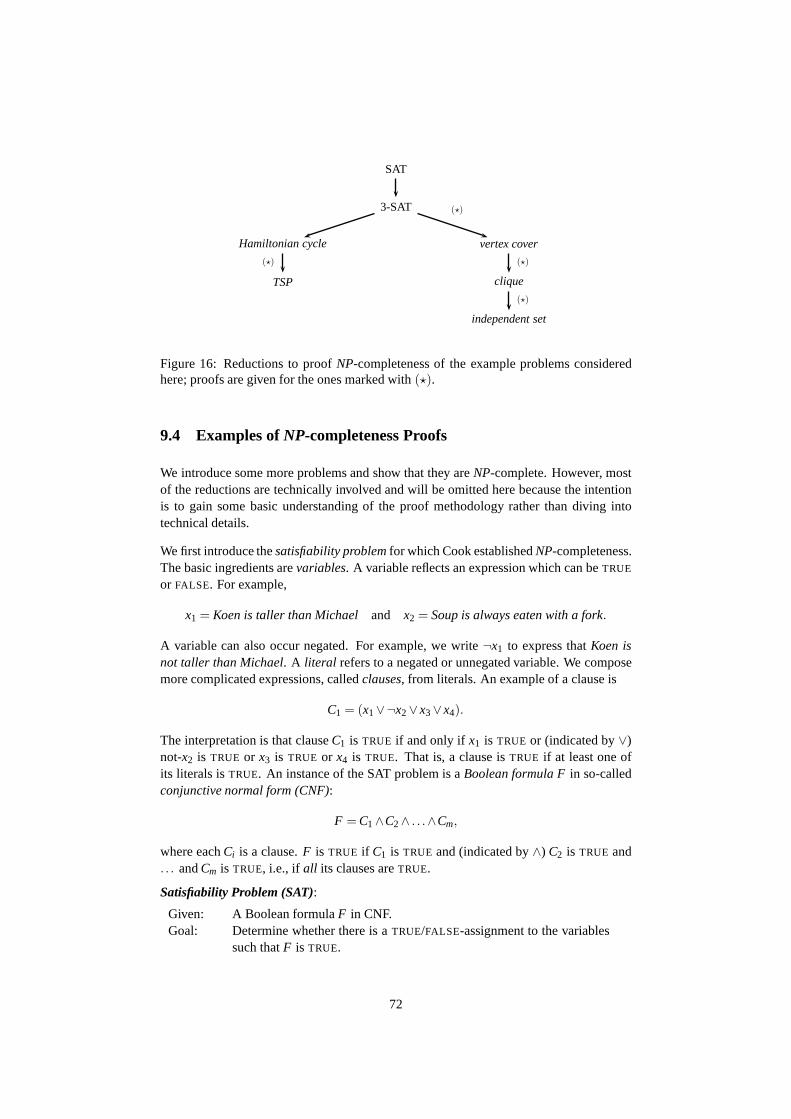
SAT
3-SAT
vertex cover
clique
independent set
Hamiltonian cycle
TSP
(⋆)
(⋆)
(⋆)
(⋆)
Figure 16: Reductions to proofNP-completeness of the example problems consideredhere; proofs are given for the ones marked with(⋆).
9.4 Examples ofNP-completeness Proofs
We introduce some more problems and show that they areNP-complete. However, mostof the reductions are technically involved and will be omitted here because the intentionis to gain some basic understanding of the proof methodologyrather than diving intotechnical details.
We first introduce thesatisfiability problemfor which Cook establishedNP-completeness.The basic ingredients arevariables. A variable reflects an expression which can beTRUE
or FALSE. For example,
x1 = Koen is taller than Michael and x2 = Soup is always eaten with a fork.
A variable can also occur negated. For example, we write¬x1 to express thatKoen isnot taller than Michael. A literal refers to a negated or unnegated variable. We composemore complicated expressions, calledclauses, from literals. An example of a clause is
C1 = (x1∨¬x2∨x3∨x4).
The interpretation is that clauseC1 is TRUE if and only if x1 is TRUE or (indicated by∨)not-x2 is TRUE or x3 is TRUE or x4 is TRUE. That is, a clause isTRUE if at least one ofits literals isTRUE. An instance of the SAT problem is aBoolean formula Fin so-calledconjunctive normal form (CNF):
F =C1∧C2∧ . . .∧Cm,
where eachCi is a clause.F is TRUE if C1 is TRUE and (indicated by∧) C2 is TRUE and. . . andCm is TRUE, i.e., if all its clauses areTRUE.
Satisfiability Problem (SAT):
Given: A Boolean formulaF in CNF.Goal: Determine whether there is aTRUE/FALSE-assignment to the variables
such thatF is TRUE.
72

Theorem 9.1. SAT is NP-complete.
The proof is involved and skipped here (the interested reader is referred to Section 15.5in [6].)
The following restriction ofsatisfiabilityis alsoNP-complete.
3-Satisfiability Problem (3-SAT):
Given: A Boolean formulaF in CNF with each clause consisting of 3 literals.Goal: Determine whether there is aTRUE/FALSE-assignment to the variables
such thatF is TRUE.
Theorem 9.2. 3-SAT is NP-complete.
The proof reducesSATto 3-SAT. We refer the reader to [6, Theorem 15.2].
We introduce some more problems and give some examples ofNP-completeness proofs.
Let G= (V,E) be an undirected graph. We need the following definitions: Acliqueof Gis a subsetV ′ of the vertices that induces a complete subgraph, i.e., for every two verticesu,v∈ V ′, (u,v) ∈ E. An independent setof G is a subsetV ′ of vertices such that no twoof them are incident to the same edge, i.e., for every two verticesu,v∈V ′, (u,v) /∈ E. Avertex coverof G is a subsetV ′ of vertices such that every edge has at least one of its twoincident vertices inV ′, i.e., for every edge(u,v) ∈ E, u,v∩V′ 6= /0.
Clique:
Given: An undirected graphG= (V,E) and an integerK.Goal: Determine whetherG contains a clique of size at leastK.
Independent Set:
Given: An undirected graphG= (V,E) and an integerK.Goal: Determine whetherG contains an independent set of size at leastK.
Vertex Cover:
Given: An undirected graphG= (V,E) and an integerK.Goal: Determine whetherG contains a vertex cover of size at mostK.
Theorem 9.3. Vertex cover is NP-complete.
Proof. We first argue thatvertex coveris in NP. A certificate of a yes-instance is a subsetV ′ ⊆ V of vertices with|V ′| ≤ K that forms a vertex cover ofG = (V,E). This can beverified in time at mostO(n+m) by checking whether each edge(u,v) ∈ E has at leastone of its incident vertices inV ′.
In order to prove thatvertex cover is NP-complete, we will show that3-SATvertex cover. Note that this is sufficient because3-SATis NP-complete.
We transform an instance of3-SATto an instance ofvertex coveras follows: Consider aBoolean formulaF in CNF with each clause having three literals. Letn andm denote the
73

x1 ¬x1 x2 ¬x2 x3 ¬x3 x4 ¬x4
C1 C2 C3
Figure 17: Illustration of the construction in the proof of Theorem9.3 for the formulaF = (x1∨x2∨¬x3)∧ (¬x1∨x2∨x4)∧ (¬x2∨x3∨x4). The red vertices constitute a vertexcover of sizeK = n+2m= 10.
number of variables and clauses ofF , respectively. We create avariable-gadgetfor eachvariablex consisting of two verticesx and¬x that are connected by an edge. Moreover,we create aclause-gadgetfor each clauseC = (l1∨ l2∨ l3) consisting of three verticesl1, l2, l3 that are connected by a triangle. Finally, we connect each vertex representing aliteral in a clause-gadget to the corresponding vertex representing the same literal in thevariable-gadget. LetG = (V,E) be the resulting graph; see Figure17 for an example.Note that this transformation can be done in polynomial time.
We show thatF is satisfiable if and only ifG has a vertex cover of size at mostK = n+2m.First note that every assignment satisfyingF can be turned into a vertex cover of sizeK: For each variable-gadget we pick the vertex that corresponds to the literal which isTRUE. This covers all edges in the variable-gadgets and their respective connections to theclause-gadgets. For each clause-gadget we choose two additional vertices so as to ensurethat all remaining edges are covered. The resulting vertex cover has sizeK = n+ 2mas claimed. Next suppose that we are given a vertex coverV ′ of G of size at mostK.Note that every vertex cover has to pick at least one vertex for every variable-gadget andtwo vertices for each clause-gadget just to cover all edges inside these gadgets. Thus,V ′ contains exactlyK vertices. The vertices inV ′ now naturally induce an assignmentas described above that satisfiesF. We conclude that yes-instances correspond under theabove reduction, which completes the proof.
Theorem 9.4. Clique is NP-complete.
Proof. We first argue thatclique is in NP. A certificate for a yes-instance is a subsetV ′
of vertices that forms a clique. To verify this, we just need to check that there is an edgebetween every pair of vertices inV ′. This can be done inO(n+m) time.
We prove thatvertex cover clique in order to establishNP-completeness ofclique. Weneed the notion of acomplement graphfor this reduction. Given a graphG= (V,E), thecomplement graph ofG is defined as the graphG= (V, E) with (u,v) ∈ E if and only if(u,v) /∈ E.
Given an instanceG= (V,E) with parameterK of vertex cover, we create the complementgraph ofG and letG with parametern−K be the respective instance ofclique. Note that
74

this mapping can be done in polynomial time by adding an edge(u,v) to E for every pairof verticesu,v∈V with (u,v) /∈ E. This takes at mostO(n2) time.
It remains to show that yes-instances correspond. We claim thatV ′ is a vertex cover inGif and only if V \V ′ is a clique inG. V ′ is a vertex cover inG if and only if every edge(u,v) ∈ E has not both its endpoints inV \V ′, or, equivalently, every edge(u,v) /∈ E hasnot both its endpoints inV \V′. The latter statement holds if and only if for every pairof verticesu,v∈V \V′ there exists an edge(u,v) ∈ E in G, which is equivalent toV \V ′
being a clique ofG. This proves the claim. We conclude thatV ′ is a vertex cover of sizeK in G if and only if V \V′ is a clique of sizen−K in G.
Theorem 9.5. Independent set is NP-complete.
Proof. We first argue thatindependent setis in NP. A certificate for a yes-instance is asubsetV ′ of vertices that forms an independent set. To verify this, wejust need to checkthat there is no edge between every pair of vertices inV ′. This can be done inO(n+m)
time.
We prove thatclique independent setin order to establishNP-completeness ofindepen-dent set. We need the notion of acomplement graphfor this reduction. Given a graphG= (V,E), the complement graph ofG is defined as the graphG= (V, E) with (u,v) ∈ Eif and only if (u,v) /∈ E.
Given an instanceG= (V,E) with parameterK of clique, we create the complement graphof G and letG with parameterK be the respective instance ofindependent set. Note thatthis mapping can be done in polynomial time by adding an edge(u,v) to E for every pairof verticesu,v∈V with (u,v) /∈ E. This takes at mostO(n2) time.
It remains to show that yes-instances correspond. We claim thatV ′ is a clique ofG if andonly if V ′ is an independent set ofG. Note thatV ′ is a clique ofG if and only if for eachpair of vertices inV ′ there is an edge inE. The latter is true if and only if for each pair ofvertices inV ′ there is no edge inE, which is equivalent toV ′ being an independent set ofG. This proves the claim. We conclude thatV ′ is a clique of sizeK in G if and only if V ′
is an independent set of sizeK in G.
Theorem 9.6. Hamiltonian cycle is NP-complete.
The proof follows by reducing3-SATto Hamiltonian cycle. The reader is referred to [6,Theorem 15.6].
Theorem 9.7. TSP is NP-complete.
Proof. We argued before thatTSP is in NP. The proof now follows trivially becauseHamiltonian cycleis a special case of TSP: Given an instanceG= (V,E) of Hamiltoniancyclewe construct an instance ofTSPas follows: LetG′ = (V,E′) be the complete graphonV and definede = 1 if e∈ E andde = 2 otherwise. Now a tour inG′ of length at mostK = n relates to a Hamiltonian cycle inG and vice versa.
75

The above proof actually shows that the restriction ofTSPin which all distances are either1 or 2 isNP-complete. BecauseTSPis in NP and it is a generalization of this problem,NP-completeness ofTSP follows immediately. The same holds true forsatisfiability:If we would not know that it isNP-complete but we would know that3-SAT is NP-complete, thenNP-completeness ofSAT followed automatically using the fact that3-SATis a special case ofSAT. While restrictions can create an easier subclass of probleminstances, generalizations always create more difficult problems. This gives sometimeseasy ways to showNP-completeness of problems.
We list some moreNP-complete problems (without proof) that are often used in reduc-tions.
2-Partition:
Given: Integerss1, . . . ,sn.Goal: Decide whether there is a setS⊆1, . . . ,n such that∑i∈Ssi =
12 ∑n
i=1si .
3-Partition:
Given: Rational numberss1, . . . ,s3n with 14 < si <
12 for everyi = 1, . . . ,3n.
Goal: Determine whether the set1, . . . ,3n can be partitioned inton tripletsS1, . . . ,Sn such that∑i∈Sk
ai = 1 for everyk= 1, . . . ,n.
Set Cover.:
Given: A universeU = 1, . . . ,n of n elements, a family ofm subsetsS1, . . . ,Sm⊆U and an integerK.
Goal: Determine whether there is a selection of at mostK subsets such thattheir union isU .
9.5 More on Complexity Theory
9.5.1 NP-hard Problems
Sometimes we may be unable to prove that a problemΠ is in NP but nevertheless canshow that all problems inNP are reducible toΠ. According to Definition9.5, Π doesnot qualify to be anNP-complete problem because it is not inNP. Yet, Π is as hard asany other problem inNP and thus probably a difficult problem. We call such problemNP-hard. An example of such a problem is theLth heaviest subset problem:
Lth Heaviest Subset Problem:
Given: Integersw1, . . . ,wn,L and a parameterK.Goal: Determine whether the weight of theLth heaviest subset of1, . . . ,n
is at leastK. (Formally, determine whether there areL distinct subsetsS1, . . . ,SL ⊆ 1, . . . ,n such thatw(Si) = ∑ j∈Si
wj ≥ K for every i =1, . . . ,L.)
It can be proven that all problems inNPare polynomial-time reducible to theLth HeaviestSubsetproblem (see [6, Theorem 16.8]). However, a proof that short certificates exist foryes-instance is non-existent. How else could we provide a certificate for a yes-instance
76

other than explicitly listingL subsets that are heavier thanK? (Note that this is not a shortcertificate becauseL can be exponential inn.)
9.5.2 Complexity Class co-NP
Another complexity class that is related toNP is the classco-NP (which stands forcom-plement of NP). Here one considers complements of decision problems. As an example,the complement ofHamiltonian cyclereads as follows:
Hamilton Cycle Complement:
Given: An undirected graphG= (V,E).Goal: Determine whetherG doesnot contain a Hamiltonian cycle.
There are noshortcertificates known for yes-instances of this problem.
Definition 9.6. A decision problemΠ belongs to the class co-NP if and only if its com-plement belongs to the classNP. Said differently, a decision problem belongs to co-NP ifevery no-instanceI ∈ I admits a certificate whose validity can be verified in polynomialtime.
It is not hard to see that every problem inP also belongs to co-NP. Thus,P⊆NP∩co-NP.Similar to theP 6= NP conjecture, it is widely believed thatNP 6= co-NP.
Theorem 9.8. If the complement of an NP-complete problem is in NP, then NP= co-NP.
Proof. Assume that the complementΠ2 of anNP-complete problemΠ2 is is in NP. Wewill show that the complementΠ1 of anarbitrary problemΠ1 ∈ NP is also inNP thusshowing thatNP= co-NP.
BecauseΠ2 is NP-complete, we know thatΠ1 is polynomial-time reducible toΠ2. Notethat the reductionϕ from Π1 to Π2 is also a polynomial-time reduction fromΠ1 to Π2.We can therefore exhibit a short certificate for every yes-instanceI1 of Π1 as follows: Wefirst transformI1 to I2 = ϕ(I1) and then use the short certificate for the yes-instanceI2(which must exist becauseΠ2 ∈ NP). We conclude thatΠ1 is in NP which finishes theproof.
Note that the above theorem also implies that if the complement of a problem inNP isalso inNP then (unlessNP= co-NP) this problem is notNP-complete. Said differently,a problem that belongs toNP∩ co-NP is unlikely to beNP-complete. As an example,consider the linear programming problemLP. Using duality theory, it is not hard to seethatLP ∈ NP∩ co-NP. BeforeLP was known to be polynomial-time solvable, it was infact the above observation that gave strong evidence to the conjecture thatLP∈ P.
Exercise 9.1.Show that LP∈ NP∩co-NP.
77
9.5.3 Pseudo-polynomiality and StrongNP-completeness
Sometimes the running time of an algorithm is polynomial in the size of the instanceandthe largest number in the input. As an example, consider theinteger knapsack problem.
Integer Knapsack Problem:
Given: Integersc1, . . . ,cn and a parameterK.Goal: Determine whether there exist integersx1, . . . ,xn such that∑n
k=1ckxk =
K.
This problem can be solved as follows: Create a directed graph G = (V,A) with K +1verticesV = 0,1, . . . ,K andO(nK) arcs:
A= (i, j) | 0≤ i < j ≤ K and j = i + ck for somek.
It is not hard to prove that an instanceI of the integer knapsackproblem is a yes-instanceif and only if there exists a path from 0 toK in G. The latter problem can be solved intime O(n+m) = O(nK). This running time isnot polynomial in the size ofI . To seethis, recall that we defined the size|I | of I to be the number of bits that are needed torepresentI in binary. Making the (reasonable) assumption thatc1, . . . ,cn < K, the sizeof I is therefore at mostO(nlogK). The running time of the algorithm is therefore notpolynomially bounded in general. However, ifK is bounded by a polynomial function ofn then the algorithm would be a polynomial-time algorithm. That is, depending on theapplication the above algorithm might indeed be consideredto be reasonably efficient,despite the fact that the problem isNP-complete (which it is).
The above observation gives rise to the following definition. Given an instanceI , letnum(I) refer to the largest integer appearing inI .
Definition 9.7. An algorithmALG for a problemΠ ispseudo-polynomialif it solves everyinstanceI ∈ I of Π in time bounded by a polynomial function in|I | and num(I).
Problems that remainNP-complete even if the largest integer appearing in its descriptionis bounded polynomially in the size of the instance is calledstrongly NP-complete.
Definition 9.8. A problemΠ is strongly NP-complete if the restriction ofΠ to instancesI ∈ I satisfying that num(I) is polynomially bounded in|I | is NP-complete.
Note that many problems that we showed to beNP-complete do not involve any numericaldata that is larger than the input size itself. For example, all graph problems such asHamiltonian cycle, clique, independent set, vertex cover, etc. satisfy num(I) = O(n) andare therefore even stronglyNP-complete by definition. In fact, alsoTSPis stronglyNP-complete because we establishedNP-completeness even for instances with distances 1 or2.
As the theorem below shows, we cannot expect to find a pseudo-polynomial algorithm fora stronglyNP-complete problem (unlessP= NP).
Theorem 9.9. There does not exist a pseudo-polynomial algorithm for a strongly NP-
78

complete problem, unless P= NP.
Proof. Let Π be a stronglyNP-complete problem and suppose thatALG is a pseudo-polynomial algorithm forΠ. Consider the restrictionΠ of Π to instancesI ∈ I thatsatisfy that num(I) is polynomially bounded in|I |. By Definition9.8, Π is NP-complete.But ALG can solve every instanceI of Π in time polynomial in|I | and num(I), which ispolynomial in|I |. This is impossible unlessP= NP.
9.5.4 Complexity ClassPSPACE
The common criterion that we used to define the complexity classesP andNPwas time:Prefers to the set of problems that are solvable in polynomialtime;NPcontains all problemsfor which yes-instances can be verified in polynomial time. There are other complexityclasses that focus on the criterionspaceinstead: The complexity classPSPACErefers tothe set of problems for which algorithms exist that only require a polynomial amount ofspace (in the size of the input).
Definition 9.9. A decision problemΠ belongs to the complexity classPSPACEif thereexists an algorithm that for every instanceI ∈ I determines whetherI is a yes-instance ora no-instance using space that is polynomially bounded in the size ofI .
Clearly, every polynomial-time algorithm cannot consume more than polynomial spaceand thusP ⊆ PSPACE. However, even exponential-time algorithms are feasible aslong as they only require polynomial space. We can use this observation to see thatNP⊆ PSPACE: Consider an arbitrary problemΠ in NP. We know that every yes-instances ofΠ admits a short certificate. We can therefore generateall potential shortcertificates one after another and verify the validity of each one. If we encounter a validcertificate throughout this procedure then we report that the instance is a yes-instance;otherwise, we report that it is a no-instance. The algorithmmay take exponential time be-cause the number of certificates to be checked might be exponential. However, it can beimplemented to use only polynomial space by deleting the previously generated certificateeach time.
As a final remark: We actually just got a tiny glimpse of the many existing com-plexity classes. There is a whole “zoo” of complexity classes; see, for example, thewiki pagehttp://qwiki.stanford.edu/index.php/ComplexityZoo if you want to learn moreabout many other complexity classes and their relations.
References
The presentation of the material in this section is based on [6, Chapters 8, 15 & 16].
79

10. Approximation Algorithms
10.1 Introduction
As we have seen, many combinatorial optimization problems are NP-hard and thus thereis very little hope that we will be able to develop efficient algorithms for these problems.Nevertheless, many of these problems are fundamental and solving them is of great im-portance. There are various ways to cope with these hardnessresults:
1. Exponential Algorithms: Certainly, using an algorithm whose running time is ex-ponential in the worst case might not be too bad after all if weonly insist onsolving instances of small to moderate size.
2. Approximation Algorithms: Approximation algorithms are efficient algorithmsthat compute suboptimal solutions with a provable approximation guarantee. Thatis, here we insist on polynomial-time computation but relaxthe condition that thealgorithm has to find an optimal solution by requiring that itcomputes a feasiblesolution that is “close” to optimal.
3. Heuristics: Any approach that solves the problem without a formal guarantee onthe quality of the solution can be considered as a heuristic for the problem. Someheuristics provide very good solutions in practice. An example of such an ap-proach islocal search: Start with an arbitrary solution and perform local improve-ment steps until no further improvement is possible. Moreover, heuristics are oftenpractically appealing because they are simple and thus easyto implement.
We give some more remarks:
Some algorithms might perform very well in practice even though their worst-case run-ning time is exponential. The simplex algorithm solving thelinear programmingproblemis an example of such an algorithm. Most real-world instances do not correspond to worst-case instances and thus “typically” the algorithms’ performance in practice is rather good.In a way, the worst-case running time viewpoint is overly pessimistic in this situation.
A very successful approach to attack optimization problemsoriginating from practicalapplications is to formulate the problem as aninteger linear programming (ILP)problemand to solve the program byILP-solvers such as CPLEX. Such solvers are nowadays veryefficient and are capable to solve large instances. Constructing the rightILP-method forsolving a given problem is a matter of smart engineering. Some ILP-problems can besolved by just running an ILP-solver; others can only be solved with the help of moresophisticated methods such as branch-and-bound, cutting-plane, column generation, etc.Especially rostering problems, like classes of universities or schedules of personnel inhospitals, are notorious for being extremely hard to solve,already for small sizes. SolvingILP-problems is an art that can be learned only in practice.
Here we will focus on approximation algorithms in order to cope with NP-hardness ofproblems. We give a formal definition of these algorithms first.
Definition 10.1. An algorithmALG for a minimization problemΠ is anα-approximationalgorithmwith α ≥ 1 if it computes for every instanceI ∈ I in polynomial time a feasible
80

solutionS∈ F whose costc(S) is at mostα times the costOPT(I) of an optimal solutionfor I , i.e.,c(S)≤ α ·OPT(I).
The definition is similar for maximization problems. Here itis more natural to assumethat we want to maximize a weight (or profit) functionw :F →R that maps every feasiblesolutionS∈ F of an instanceI ∈ I to some real value.
Definition 10.2. An algorithmALG for a maximization problemΠ is anα-approximationalgorithmwith α ≥ 1 if it computes for every instanceI ∈ I in polynomial time a feasiblesolutionS∈ F whose weight (or profit)w(S) is at least1α times the weightOPT(I) of anoptimal (i.e., maximum weight) solution forI , i.e.,w(S)≥ 1
α ·OPT(I).
Note that we would like to design approximation algorithms with the approximation ra-tio α being as small as possible. A lot of research in theoretical computer science anddiscrete mathematics is dedicated to the finding of “good” approximation algorithms forcombinatorial optimization problems.
10.2 Approximation Algorithm for Vertex Cover
We start with an easy approximation algorithm for thevertex coverproblem, which hasbeen introduced before: Given a graphG = (V,E), find a vertex coverV ′ ⊆V of small-est cardinality. Recall that we showed that the decision variant of vertex coveris NP-complete.
One of the major difficulties in the design of approximation algorithms is to come up witha good estimate for the optimal solution costOPT(I). (We will omit I subsequently.)Recall that a matchingM is a subset of the edges having the property that no two edgesshare a common endpoint. We call a matchingM maximumif the cardinality ofM ismaximum; we call itmaximalif it is inclusion-wisemaximal, i.e., we cannot add anotheredge toM without rendering it infeasible. Note that a maximum matching is a maximalone but not vice versa.
Lemma 10.1. Let G= (V,E) be an undirected graph. If M is a matching of G thenOPT≥ |M|.
Proof. Consider an arbitrary vertex coverV ′ of G. Every matching edge(u,v) ∈M mustbe covered by at least one vertex inV ′, i.e.,u,v∩V′ 6= /0. Because the edges inM donot share any endpoints, we have|V ′| ≥ |M|.
We conclude that we can derive an easy 2-approximation algorithm for vertex coverasfollows:
Theorem 10.1. Algorithm14 is a2-approximation algorithm for vertex cover.
Proof. Clearly, the running time of Algorithm14 is polynomial because we can find amaximal matching in time at mostO(n+m). The algorithm outputs a feasible vertex
81

Input : Undirected graphG= (V,E).Output : Vertex coverV ′ ⊆V.
1 Find a maximal matchingM of G.2 Output the setV ′ of matched vertices.
Algorithm 14: Approximation algorithm forvertex cover.
cover because of the maximality ofM. To see this, suppose that the resulting setV ′ isnot a vertex cover. Then there is an edge(u,v) with u,v /∈ V ′ and thus bothu andv areunmatched inM. We can then add the edge(u,v) to M and obtain a feasible matching,which contradicts the maximality ofM. Finally, observe that|V ′| = 2|M| ≤ 2OPT byLemma10.1.
Note that it suffices to compute a maximal (not necessarily maximum) matching in Algo-rithm 14, which can be done in linear timeO(m).
An immediate question that comes to ones mind is whether the approximation ratio is bestpossible. This indeed involves two kinds of questions in general:
1. Is the approximation ratioα of the algorithm tight?2. Is the approximation ratioα of the algorithm best possible forvertex cover?
The first question essentially asks whether the analysis of the approximation ratio is tight.This is usually answered by exhibiting an example instance for which the algorithm com-putes a solution whose cost isα times the optimal one. The second one asks for muchmore: Can one show that there is no approximation algorithm with approximation ratioα−ε for everyε > 0? Such aninapproximability resultusually relies on some conjecturesuch as thatP 6= NP.
Lets first argue that the approximation ratio of Algorithm14 is indeed tight.
Example 10.1.Consider a complete bipartite graph withn vertices on each side. Theabove algorithm will pick all 2n vertices, while picking one side of the bipartition con-stitutes an optimal solution of cardinalityn. The approximation ratio of 2 is thereforetight.
The answer to the second question is not clear, despite intensive research. The currentlybest known lower bound on the inapproximability ofvertex coveris as follows (statedwithout proof).
Theorem 10.2.Vertex cover cannot be approximated within a factor of1.3606, unlessP= NP.
10.3 Approximation Algorithms for TSP
As introduced before, thetraveling salesman problemasks for the computation of a short-est tour in a given graphG= (V,E) with non-negative edge costsc : E→R+.
82
We first show the following inapproximability result.
Theorem 10.3.For any polynomial-time computable functionα(n), TSP cannot be ap-proximated within a factor ofα(n), unless P= NP.
Proof. Suppose we have an algorithmALG that approximatesTSPwithin a factorα(n).We show that we can useALG to decide in polynomial time whether a given graph has aHamiltonian cycle or not, which is impossible unlessP= NP.
Let G = (V,E) be a given graph onn vertices. We extendG to a complete graph andassign each original edge a cost of 1 and every other edge a cost of nα(n). Run theα(n)-approximation algorithmALG on the resulting instance. We claim thatG containsa Hamiltonian cycle if and only if the TSP tour computed byALG has cost less than orequal tonα(n).
SupposeG has a Hamiltonian cycle. Then the optimal TSP tour in the extended graphhas costn. The approximate TSP tour computed byALG must therefore have cost lessthan or equal tonα(n). SupposeG does not contain a Hamiltonian cycle. Then everyfeasible TSP tour in the extended graph must use at least one edge of costnα(n), i.e., thecost of the tour is greater thannα(n) (assuming thatG has at leastn≥ 2 vertices). Thus,the cost of the approximate TSP tour computed byALG is greater thannα(n). The claimfollows.
The above inapproximability result is extremely bad news. The situation changes if weconsider themetric TSPproblem.
Metric Traveling Salesman Problem (Metric TSP):
Given: An undirected complete graphG = (V,E) with non-negative costsc :E → R+ satisfying thetriangle inequality, i.e., for everyu,v,w ∈ V,cuw≤ cuv+ cvw.
Goal: Compute a tour inG that minimizes the total cost.
Themetric TSPproblem remainsNP-complete: Recall that we showed that theTSPprob-lem isNP-complete by reducingHamiltonian Cycleto this problem. The reduction onlyused edge costs 1 and 2. Note that such edge costs always constitute a metric. Thus, thesame proof shows thatmetric TSPis NP-complete.
We next derive two constant factor approximation algorithms for this problem.
Given a subsetQ⊆ E of the edges, we definec(Q) as the total cost of all edges inQ, i.e.,c(Q) = ∑e∈Q ce.
The following lemma establishes a lower bound on the optimalcost:
Lemma 10.2. Let T be a minimum spanning tree of G. ThenOPT≥ c(T).
Proof. Consider an optimalTSPtour and remove an arbitrary edge from this tour. Weobtain a spanning tree ofG whose cost is at mostOPT. The cost ofT is thus at mostOPT.
83

This lemma leads to the following idea:5
Input : Complete graphG= (V,E) with non-negative edge costsc : E→R+
satisfying the triangle inequality.Output : TSPtour ofG.
1 Compute a minimum spanning treeT of G.2 Double all edges ofT to obtain a Eulerian graphG′.3 Extract a Eulerian tourC′ from G′.4 TraverseC′ and short-cut previously visited vertices.5 Output the resulting tourC.
Algorithm 15: Approximation algorithm formetric TSP.
Theorem 10.4. Algorithm15 is a2-approximation algorithm for metric TSP.
Proof. Note that the algorithm has polynomial running time. Also, the returned tour is aTSP tour by construction. Because edge costs satisfy the triangle inequality, the tourCresulting from short-cutting the Eulerian tourC′ in Algorithm 15 has cost at most 2c(T),whereT is the minimum spanning tree computed in Step1. By Lemma10.2, the cost ofC is thus at most 2OPT.
We can actually derive a better approximation algorithm by refining the idea of Algo-rithm 15. Note that the reason for doubling the edges of a minimum spanning treeT wasthat we would like to obtain a Eulerian graph from which we canthen extract a Euleriantour. Are there better ways to construct a Eulerian graph starting with a minimum span-ning treeT? Certainly, we only have to take care of the odd degree vertices, sayV ′, of T.Note that in a tree there must be an even number of odd degree vertices.
So one way of making these odd degree vertices become even degree vertices is to addthe edges of a perfect matching onV ′ to T. Intuitively, we would like to keep the totalcost of the augmented tree small and thus compute a minimum cost perfect matching. Asthe following lemma shows, the cost of this matching can be related to the optimal cost.
Lemma 10.3. Let V′ ⊆V be a subset containing an even number of vertices. Let M be aminimum cost perfect matching on V′. ThenOPT≥ 2c(M).
Proof. Consider an optimalTSPtourC of lengthOPT. Traverse this tour and short-cut allvertices inV \V′. Because of the triangle inequality, the resulting tourC′ onV ′ has lengthat mostOPT. C′ can be seen as the union of two perfect matchings onV ′. The cheapermatching of these two must have cost at most1
2OPT. We conclude that a minimum costperfect matchingM onV ′ has cost at most12OPT.
We combine the above observations in the following algorithm, which is also known asChristofides’ algorithm.
5Recall that aEulerian graphis a connected graph that has no vertices of odd degree. AEulerian tour is acycle that visits every edge of the graph exactly once. Givena Eulerian graph, we can always find a Euleriantour.
84

Input : Complete graphG= (V,E) with non-negative edge costsc : E→R+
satisfying the triangle inequality.Output : TSPtour ofG.
1 Compute a minimum spanning treeT of G.2 Compute a perfect matchingM on the odd degree verticesV ′ of T.3 CombineT andM to obtain a Eulerian graphG′.4 Extract a Eulerian tourC′ from G′.5 TraverseC′ and short-cut previously visited vertices.6 Output the resulting tourC.
Algorithm 16: Approximation algorithm formetric TSP.
Theorem 10.5. Algorithm16 is a 32-approximation algorithm for metric TSP.
Proof. Note that the algorithm can be implemented to run in polynomial time (computinga perfect matching in an undirected graph can be done in polynomial time). The prooffollows because the Eulerian graphG′ has total costc(T)+c(M). Because of the triangle-inequality, short-cutting the Eulerian tourC′ does not increase the cost. The resultingtour C has thus cost at mostc(T)+ c(M), which by Lemmas10.2and10.3 is at most32OPT.
The algorithm is tight (example omitted). Despite intensive research efforts, this is stillthe best known approximation algorithm for themetric TSPproblem.
10.4 Approximation Algorithm for Steiner Tree
We next consider a fundamental network design problem, namely the Steiner tree prob-lem. It naturally generalizes theminimum spanning tree problem:
Steiner Tree Problem:
Given: An undirected graphG= (V,E) with non-negative edge costsc : E→R+ and a set of terminal nodesR⊆V.
Goal: Compute a minimum cost treeT in G that connects all terminals inR.
The nodes inR are usually calledterminals; those inV \R are calledSteinernodes. TheSteiner treeproblem thus asks for the computation of a minimum cost tree,also calledSteiner tree, that spans all terminals inR and possibly some Steiner nodes. The decisionvariant of the problem isNP-complete. Note that if we knew the setS⊆V \R of Steinernodes that are included in an optimal solution, then we couldsimply compute an optimalSteiner tree by computing a minimum spanning tree on the vertex setR∪S in G. Thus,the difficulty of the problems is that we do not know which Steiner nodes to include.
We first show that we can restrict our attention without loss of generality to the so-calledmetric Steiner tree problem. In the metric version of the problem, we are given acom-pletegraphG= (V,E) with non-negative edge costsc : E→ R+ that satisfy thetriangle
85

inequality, i.e., for everyu,v,w∈V, cuw≤ cuv+ cvw.
Given a subsetQ⊆ E of the edges, we definec(Q) as the total cost of all edges inQ, i.e.,c(Q) = ∑e∈Q ce.
Theorem 10.6.There is an approximation preserving polynomial-time reduction fromSteiner tree to metric Steiner tree.
Proof. Consider an instanceI = (G,c,R) of theSteiner tree problemconsisting of a graphG = (V,E) and edge costsc : E → R+. We construct a corresponding instanceI ′ =(G′,c′,R) of metric Steiner treeas follows. LetG′ = (V,E′) be the complete undirectedgraph on vertex setV and letE′ be its set of edges. Define the costc′e of edgee= (u,v) ∈E′ as the cost of a shortest path betweenu andv in G. (G′,c′) is called themetric closureof (G,c). The set of terminals inI andI ′ is identical.
Suppose we are given a Steiner treeT in G. Then the cost of the Steiner treeT in (G′,c′)can only be smaller. Next suppose we are given a Steiner treeT ′ of (G′,c′). Each edgee= (u,v) ∈ T ′ corresponds to a shortestu,v-path inG. The subgraph ofG induced by alledges inT ′ connects all terminals inRand has cost at mostc′(T ′) but may contain cyclesin general. If so, remove edges to obtain a treeT in G. Clearly,c(T)≤ c′(T ′).
In light of Theorem10.6, we concentrate on themetric Steiner tree problemsubsequently.
As mentioned before, the key to derive good approximation algorithms for a problem isto develop good lower bounds on the optimal costOPT. One such lower bound is thefollowing:
Lemma 10.4. Let T be a minimum spanning tree on the terminal set R of G. ThenOPT≥12c(T).
Proof. Consider an optimal Steiner tree of costOPT. By doubling the edges of this tree,we obtain a Eulerian graph of cost 2OPT that connects all terminals inR and a (possiblyempty) subset of Steiner vertices. Find a Eulerian tourC′ in this graph (e.g., by traversingvertices in their depth-first search order). We obtain a Hamiltonian cycleC on R bytraversingC′ and short-cutting Steiner vertices and previously visitedterminals. Becauseof the triangle inequality, this short-cutting will not increase the cost and the cost ofC isthus at mostc(C′) = 2OPT. Delete an arbitrary edge ofC to obtain a spanning tree onRof cost at most 2OPT. The cost of a minimum spanning treeT on R is less than or equalto the cost of this spanning tree, which is at most 2OPT.
Lemma10.4gives rise to the following approximation algorithm.
Theorem 10.7. Algorithm17 is a2-approximation algorithm for metric Steiner tree.
Proof. Certainly, the algorithm has polynomial running time and outputs a feasible solu-tion. The approximation ratio of 2 follows directly from Lemma10.4.
86

Input : Complete graphG= (V,E) with non-negative edge costsc : E→R+
satisfying the triangle inequality and a set of terminal verticesR⊆V.Output : Steiner treeT onR.
1 Compute a minimum spanning treeT on terminal setR.2 OutputT.
Algorithm 17: Approximation algorithm formetric Steiner tree.
Figure 18: Example graph
The analysis of Algorithm10.4 is tight as the followingexample shows:
Example 10.2. Consider a complete graph that consists ofk outer terminal verticesR= t1, . . . , tk that are connectedto one inner Steiner vertex; see Figure18 for an examplewith k = 8. The edges to the Steiner vertex have cost 1;all remaining ones have cost 2. Note that these edge costssatisfy the triangle inequality. A minimum spanning treeon the gray vertices has total cost 2(k−1) while the min-imum Steiner tree has costk. That is, the approximation ratio of Algorithm10.4on thisinstance is 2−2/k. As k goes to infinity, this ratio approaches 2.
There are much better approximation algorithms for this problem. The current best ap-proximation ratio is 1.386. Inapproximability results show that the problem cannot beapproximated arbitrarily well. In particular, there is no 96/95-approximation algorithmfor themetric Steiner treeproblem.
10.5 Approximation Scheme forKnapsack
We next consider theknapsack problem:
Knapsack Problem:
Given: A setN = 1, . . . ,n of n items with each itemi ∈ N having a profitpi ∈ Z+ and a weightwi ∈ Z+, and a knapsack whose (weight) capacityis B∈ Z+.
Goal: Find a subsetX ⊆ N of items whose total weightw(X) = ∑i∈X wi is atmostB such that the total profitp(X) = ∑i∈X pi is maximum.
We will assume without loss of generality thatwi ≤ B for everyi ∈ N and thatpi > 0 foreveryi ∈ N; items not satisfying one of these conditions can safely be ignored.
Theknapsack problemis NP-hard and we therefore seek a good approximation algorithmfor the problem. As we will see, we can even derive anapproximation schemefor thisproblem:
Definition 10.3. An algorithmALG is anapproximation schemefor a maximization prob-lem Π if for every given error parameterε > 0 and every instanceI ∈ I, it computes a
87

feasible solutionS∈ F of profit p(S)≥ (1− ε)OPT(I). An approximation schemeALG
is a
• polynomial time approximation scheme (PTAS)if for every fixedε > 0 its runningtime is polynomial in the size of the instanceI ;• fully polynomial time approximation scheme (FPTAS)if its running time is poly-
nomial in the size of the instanceI and 1ε .
Note that the running time of a PTAS might grow exponentiallyin 1ε , e.g., likeO(21/εn2),
while this is not feasible for a FPTAS.
10.5.1 Dynamic Programming Approach
The algorithm is based on the followingdynamic programmingapproach. Let the max-imum profit of an item in a given instanceI be denoted byP(I) (we will omit I subse-quently). A trivial upper bound on the total profit that any solution for I can achieve isnP. Define for everyi ∈N and everyp∈ 0, . . . ,nP:
A(i, p) = minimum weight of a subsetS⊆ 1, . . . , i whose profitp(S) is exactlyp.
Let A(i, p) = ∞ if no such set exists. Suppose we were able to computeA(i, p). We canthen easily determine the total profit of an optimal solution:
OPT= maxp∈ 0, . . . ,nP | A(n, p)≤ B.
Clearly, A(1, p1) = w1 and A(1, p) = ∞ for every p > 0 with p 6= p1. We further setA(i,0) = 0 for everyi ∈ N and implicitly assume thatA(i, p) = ∞ for everyp< 0. Letssee how to computeA(i + 1, p) for i ≥ 1 andp > 0. There are two options: either weinclude itemi +1 into the knapsack or not. If we include itemi +1, then it contributesa profit of pi+1 and thus the minimum weight of a subset of1, . . . , i +1 with profit pis equal to the minimum weightA(i, p− pi+1) of the firsti items yielding profitp− pi+1
plus the weightwi+1 of item i+1. If we do not include itemi+1, thenA(i+1, p) is equalto A(i, p). Thus
A(i +1, p) = minwi+1+A(i, p− pi+1), A(i, p). (17)
We can therefore compute the table of entriesA(i, p) with i ∈ N and p ∈ 0, . . . ,nP intimeO(n2P).
Note that the dynamic program haspseudo-polynomialrunning time (cf. Definition9.7),i.e., the running time of the algorithm is polynomial in the size of the instance (heren) andthe largest integer appearing in the instance (hereP). However, we can use this pseudo-polynomial algorithm in combination with the following rounding idea to obtain a fullypolynomial-time approximation scheme for this problem.
88

Input : A setN = 1, . . . ,n of items with a profitpi ∈ Z+ and a weightwi ∈ Z+ forevery itemi ∈ N and a knapsack capacityB∈ Z+.
Output : SubsetX′ ⊆ N of items.
1 Sett =⌊
log10
( εPn
)⌋
.2 Definetruncated profitspi = ⌊pi/10t⌋ for everyi ∈ N.3 Use the dynamic program (17) to compute an optimal solutionX′ for the
knapsack instance(N,(pi),(wi),B).4 OutputX′.
Algorithm 18: Approximation scheme forknapsack.
10.5.2 Deriving a FPTAS forKnapsack
Note that the above algorithm runs in polynomial time if all profits of the items are smallnumbers, e.g., if they are polynomially bounded inn. The key idea behind deriving aFPTAS is to ignore a certain number (depending on the error parameterε) of least sig-nificant bits of the items’ profits. The modified profits can be viewed as numbers thatare polynomially bounded in|I | and 1
ε . As a consequence, we can compute an optimalsolution for the modified profits in time polynomial in|I | and 1
ε using the above dynamicprogram. Because we only ignore the least significant bits, this solution will be a(1− ε)-approximate solution with respect to the original profits. Subsequently, we elaborate onthis idea in more detail.
Suppose we truncate the lastt digits of each item’s profit. That is, define thetruncatedprofit pi of item i as pi = ⌊pi/10t⌋. Now use the dynamic program above to computean optimal solutionX′ for the instance with truncated profits. This takes time at mostO(n2P/10t).
Certainly,X′ may be sub-optimal for the original problem, but its total profit relates to theone of an optimal solutionX for the original problem as follows:
∑i∈X′
pi ≥ ∑i∈X′
10t pi ≥ ∑i∈X
10t pi ≥ ∑i∈X
(pi−10t)≥ ∑i∈X
pi−n10t .
Here, the first and third inequalities hold because of the definition of truncated profits. Thesecond inequality follows from the optimality ofX′. Thus, the total profit ofX′ satisfies
p(X′)≥ p(X)−n10t =OPT
(
1− n10t
OPT
)
≥ OPT
(
1− n10t
P
)
.
Note that the last inequality holds becauseOPT ≥ P. Suppose we wish to obtain anapproximation ratio of 1− ε. We can accomplish this by lettingt be the smallest integersuch thatn10t/P≤ ε, or, equivalently,
t =
⌊
log10
(
εPn
)⌋
.
With this choice, the running time of the dynamic program isO(n2P/10t) = O(n3/ε).
89

That is, for anyε > 0 we have an(1−ε)-approximation algorithm whose running time ispolynomial in the size of the instance and1
ε .
We summarize the result in the following theorem.
Theorem 10.8. Algorithm 18 is a fully polynomial time approximation scheme for theknapsack problem.
References
The presentation of the material in this section is based on [9, Chapters 1 & 3].
90

References
[1] R. K. Ahuja, T. L. Magnanti, and J. B. Orlin,Network flows: Theory, algorithms, andapplications, Prentice Hall, New Jersey, 1993.
[2] W. J. Cook, W. H. Cunningham, W. R. Pulleyblank, and Schrijver A., Combinatorialoptimization, Wiley, 1998.
[3] T. H. Cormen, C. Leiserson, R. L. Rivest, and C. Stein,Introduction to algorithms,MIT Press, 2001.
[4] M. R. Garey and D. S. Johnson,Computers and intractability: A guide to the theoryof NP-completeness, W. H. Freeman & Co., New York, NY, USA, 1979.
[5] B. Korte and J. Vygen,Combinatorial optimization: Theory and algorithms,Springer, 2008.
[6] C. H. Papadimitriou and K. Steiglitz,Combinatorial optimization: Algorithms andcomplexity, Prentice-Hall, Inc., Upper Saddle River, NJ, USA, 1982.
[7] A. Schrijver,Combinatorial optimization: Polyhedra and efficiency, Springer, Berlin,Heidelberg, New York, 2003.
[8] R. E. Tarjan,Data structures and network algorithms, Society for Industrial and Ap-plied Mathematics, Philadelphia, Pennsylvania, 1983.
[9] Vijay V. Vazirani, Approximation algorithms, Springer, Berlin, Heidelberg, New-York, 2001.