lecture notes for astrophysics i spring...
TRANSCRIPT

Lecture Notes for Astrophysics I
Spring 2011
Lecturer: Professor Lam HuiTranscriber: Alexander Chen
July 8, 2011
Contents
1 Lecture 1 31.1 Gravitational Lensing . . . . . . . . . . . . . . . . . . . . . . . . . . . . . . . . . . . . . . . 31.2 Example . . . . . . . . . . . . . . . . . . . . . . . . . . . . . . . . . . . . . . . . . . . . . . . 4
2 Lecture 2 62.1 Gravitational Lensing Continued . . . . . . . . . . . . . . . . . . . . . . . . . . . . . . . . . 62.2 Magnification in Gravitational Lensing . . . . . . . . . . . . . . . . . . . . . . . . . . . . . . 62.3 Stellar Structure . . . . . . . . . . . . . . . . . . . . . . . . . . . . . . . . . . . . . . . . . . 8
3 Lecture 3 93.1 Stellar Structure Continued . . . . . . . . . . . . . . . . . . . . . . . . . . . . . . . . . . . . 93.2 Stellar Structure Equations . . . . . . . . . . . . . . . . . . . . . . . . . . . . . . . . . . . . 93.3 Virial Theorem . . . . . . . . . . . . . . . . . . . . . . . . . . . . . . . . . . . . . . . . . . . 103.4 Stellar Structure Equations Continued . . . . . . . . . . . . . . . . . . . . . . . . . . . . . . 10
4 Lecture 4 144.1 Opacity . . . . . . . . . . . . . . . . . . . . . . . . . . . . . . . . . . . . . . . . . . . . . . . 144.2 Energy Generation . . . . . . . . . . . . . . . . . . . . . . . . . . . . . . . . . . . . . . . . . 144.3 Explanation of the Main Sequence . . . . . . . . . . . . . . . . . . . . . . . . . . . . . . . . 17
5 Lecture 5 205.1 Main-Sequence Continued . . . . . . . . . . . . . . . . . . . . . . . . . . . . . . . . . . . . . 205.2 White Dwarves . . . . . . . . . . . . . . . . . . . . . . . . . . . . . . . . . . . . . . . . . . . 21
6 Lecture 6 266.1 Chandrasekar Limit . . . . . . . . . . . . . . . . . . . . . . . . . . . . . . . . . . . . . . . . 266.2 Coulomb Effect . . . . . . . . . . . . . . . . . . . . . . . . . . . . . . . . . . . . . . . . . . . 276.3 Inverse β-decay . . . . . . . . . . . . . . . . . . . . . . . . . . . . . . . . . . . . . . . . . . . 28
1
7 Lecture 7 307.1 Neutron Stars . . . . . . . . . . . . . . . . . . . . . . . . . . . . . . . . . . . . . . . . . . . . 317.2 Stellar Structure for Neutron Star . . . . . . . . . . . . . . . . . . . . . . . . . . . . . . . . 33
8 Lecture 8 358.1 Neutron Stars Mass Limit . . . . . . . . . . . . . . . . . . . . . . . . . . . . . . . . . . . . . 358.2 Neutron Star Magnetic Field - Dipole Model . . . . . . . . . . . . . . . . . . . . . . . . . . 368.3 Beyond the Dipole Model . . . . . . . . . . . . . . . . . . . . . . . . . . . . . . . . . . . . . 38
9 Lecture 9 409.1 Black Holes . . . . . . . . . . . . . . . . . . . . . . . . . . . . . . . . . . . . . . . . . . . . . 40
10 Lecture 10 4510.1 Kerr Black Hole Continued . . . . . . . . . . . . . . . . . . . . . . . . . . . . . . . . . . . . 4510.2 Accretion on the Black Hole . . . . . . . . . . . . . . . . . . . . . . . . . . . . . . . . . . . . 47
11 Lecture 11 4911.1 Generation of Gravitational Waves . . . . . . . . . . . . . . . . . . . . . . . . . . . . . . . . 49
12 Lecture 12 5412.1 Calculation of Gravitational Wave Production . . . . . . . . . . . . . . . . . . . . . . . . . . 5412.2 Energy of Graviton . . . . . . . . . . . . . . . . . . . . . . . . . . . . . . . . . . . . . . . . . 55
13 Lecture 13 5813.1 Gravitational Wave Braking . . . . . . . . . . . . . . . . . . . . . . . . . . . . . . . . . . . . 5813.2 Hawking Radiation . . . . . . . . . . . . . . . . . . . . . . . . . . . . . . . . . . . . . . . . . 5913.3 Crush Course on Quantum Field Theory . . . . . . . . . . . . . . . . . . . . . . . . . . . . . 61
14 Lecture 14 63
2
Astrophysics I Lecture 1
1 Lecture 1
The study of astrophysics is divided into two parts. One is cosmology, which studies the universe as awhole, and the other one is just astrophysics which considers the objects in the universe individually. Wewill talk about almost everything in astrophysics, but not cosmology. The subject we are going to coverspans a wide range, so there is no one textbook that can cover everything. We want to use the first coupleof weeks to cover gravitational lensing and gravitational waves, especially how the latter is produced. Afterthat we will be talking about stars, or main-sequence stars, and then will go to compact objects like whitedwarves and neutron stars, and finally get to black holes. In the end, just for fun, we will talk aboutHawking radiation, which is the quantum aspects of black holes.
1.1 Gravitational Lensing
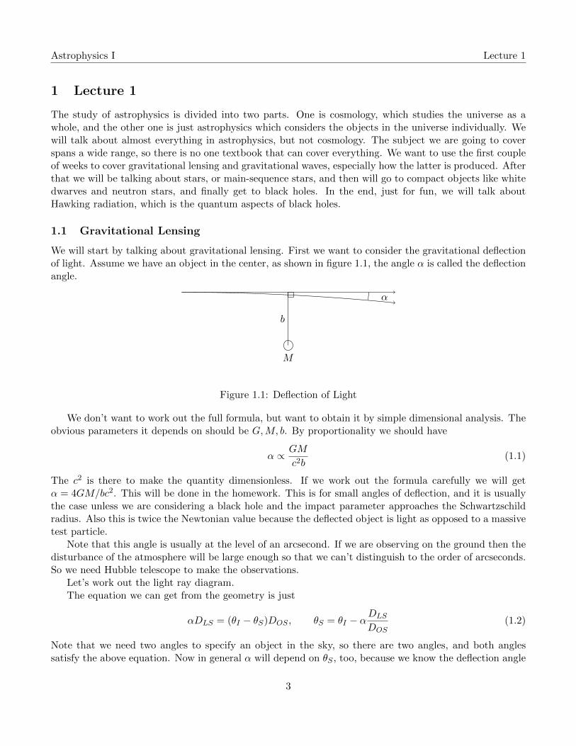
We will start by talking about gravitational lensing. First we want to consider the gravitational deflectionof light. Assume we have an object in the center, as shown in figure 1.1, the angle α is called the deflectionangle.
α
M
b
Figure 1.1: Deflection of Light
We don’t want to work out the full formula, but want to obtain it by simple dimensional analysis. Theobvious parameters it depends on should be G,M, b. By proportionality we should have
α ∝ GM
c2b(1.1)
The c2 is there to make the quantity dimensionless. If we work out the formula carefully we will getα = 4GM/bc2. This will be done in the homework. This is for small angles of deflection, and it is usuallythe case unless we are considering a black hole and the impact parameter approaches the Schwartzschildradius. Also this is twice the Newtonian value because the deflected object is light as opposed to a massivetest particle.
Note that this angle is usually at the level of an arcsecond. If we are observing on the ground then thedisturbance of the atmosphere will be large enough so that we can’t distinguish to the order of arcseconds.So we need Hubble telescope to make the observations.
Let’s work out the light ray diagram.The equation we can get from the geometry is just
αDLS = (θI − θS)DOS , θS = θI − αDLS
DOS(1.2)
Note that we need two angles to specify an object in the sky, so there are two angles, and both anglessatisfy the above equation. Now in general α will depend on θS , too, because we know the deflection angle
3

Astrophysics I Lecture 1
O
S
I
θSθI
α
L
DOL DLS
Figure 1.2: Light Ray of Deflection
is dependent on the impact parameter, so this equation is not linear in general. Because this equation hasmultiple solutions, there will be multiple images for the same object.
1.2 Example
Let’s consider an example of a point lense. We should have the following equation
αi =4GM
c2 |θI |DOLθiI (1.3)
This is just from the deflection equation above and we have taken the impact parameter to be b = DOLθI .Now we can put this into the above equation and get and equation for the image position
θS = θI −4GM
c2DOL
DLS
DOS
1
θI= θI − θ2
E
1
θI(1.4)
The quantity θE is called the Einstein angle. It is apparent that this equation is a quadratic one and hastwo solutions
θI =θS ±
√θ2S + 4θ2
E
2(1.5)
The Einstein angle has a nice interpretation as when θS = 0 then the image position will be exactly atthe Einstein angle. Typical numbers for the Einstein angle are about θE ∼ 3′′ for M = 1012Msun andD = 1 Gpc.
Now there is something puzzling about this. If this result is always true, why don’t we see a lot ofdouble imaging in the sky? The answer lies in the magnitude of the image. Actually the luminosity of theimage is also contained inside the lense equation. When the source angle is large, but not so large that thesmall angle approximation breaks down, then we will expect that one of the images will just be θI ≈ θSwhich is just light directly from the source. However we have another solution which is a negative rootwith
θI =θS −
√θ2S + 4θ2
E
2≈ −
θ2E
θS(1.6)
4
Astrophysics I Lecture 1
This is usually the case because we rarely see the objects in the sky to line up exactly. We can determinethe apparent magnitude of this image by studying the so called magnification matrix defined by
Aij =∂θiI∂θjS
(1.7)
The fact that this matrix is not identity will tell us how the shape of the image becomes distorted fromthe original shape. Our hope is that this matrix will tell us that the image we considered above will besignificantly demagnified. We can figure it out by taking derivative directly on the lense equation (1.2).We will finish this next time.
5
Astrophysics I Lecture 2
2 Lecture 2
2.1 Gravitational Lensing Continued
We will postpone the discussion of gravitational waves because of prerequisite issues. So we will first discussstellar structure, namely main-sequence stars, white dwarves, neutron stars, etc. Recall last time we weretalking about gravitational lensing. The lensing equation was obtained from geometry
αiDLS = (θiI − θiS)DOS , θiS = θiI − αiDLS
DOS(2.1)
Note that any object in the sky is characterized by two angles, so we have an index on the above equation.Combined with the deflection of light by gravitation we get the image equation
θiS = θiI −θ2E∣∣θiI ∣∣ θiI (2.2)
where θE is the Einstein angle. Note that this equation tells us that there are always at least two images ifwe approximate the lensing object as a point lense. The Einstein angle is the image angle when the sourceangle becomes zero.
When θS is large, but not so large that the small-angle approximation breaks down, then one imagewill be at approximately the same position as θS , and the other image will be very close to the lensingobject at the other side. However of the source angle is very close to zero, then one image will be justoutside of the Einstein angle, and the other will be just inside of the angle. Today we want to work outthe apparent magnitude of the images.
2.2 Magnification in Gravitational Lensing
In nature none of the realistic objects is a point source, so any object in the sky should span some angle∆θ. We want to figure out the relation between ∆θI and ∆θS . We define the following matrix
Aij =∂θiS∂θjI
(2.3)
The inverse of this matrix is basically (A−1
)ij=∂θiI∂θjS
(2.4)
This matrix is called the magnification matrix, because by definition we have the following relation
∆θiI =(A−1
)ij∆θjS (2.5)
Note that this matrix not only tells us the magnification, but also tells us the distortion of the image inany direction. The reason we defined the matrix indirectly is because the matrix Aij is easier to calculate:just differentiate the lensing equation. The magnification matrix is always symmetric, although it is notvery obvious in the way we define it. The area spanned by the image is the determinant of A−1 times thearea spanned by the source.
6

Astrophysics I Lecture 2
Let’s take the derivative of the lensing equation and calculate the matrix Aij
Aij =∂θiS∂θjI
= δij −θ2E
|θI |2δij + 2θ2
E
θiIθjI
|θI |4
= δij(
1−θ2E
|θI |2
)+ 2θ2
E
θiIθjI
|θI |4
(2.6)
Now if we choose ij to be among x, y, and choose the axis such that the source and image and lensingpoint are all on the y axis, so θxI = 0. Then the matrix becomes diagonal and we have
Aij =
(1− θ2
E/ |θI |2 0
0 1 + θ2E/ |θI |
2
)(2.7)
Note that as one entry is larger than 1 and the other is smaller than 1, the image is squeezed in onedirection and stretched in the other direction. The magnification matrix is actually
A−1 =
(1
1−θ2E/θ2I
0
0 11+θ2E/θ
2I
)(2.8)
Now if our source looks like a circle, then it will be stretched in the x direction and squeezed in the ydirection and the image will look like an ellipse. Now in the first case where the image is very close tothe source, we know that both θS and θI are much larger than θE , so the stretch and squeeze in bothdirections are very tiny. Now if we consider θI close to zero, then θE/θI 1, and the first entry in theabove matrix will be negative. The magnitude of both entries become much smaller than 1, so the imagewill be significantly demagnified, and we can hardly observe these images. This is the weak-lensing limit.
The other limit is the strong-lensing limit. In this limit θS is very close to 0 and θI of both images willbe close to the Einstein angle and one is outside Einstein ring while the other is inside. Under this limitwe can see that θE/θI ≈ 1. Then the first entry in the magnification matrix is very large while the secondentry is close to 1/2. So the image is strongly stretched in the x direction. So the images will look likewhat is shown in figure 2.1.
Figure 2.1: Strong lensing limit
Note that the matrix element blows up when θS becomes 0. Now this is resolved because we don’treally have a point source, and the magnification should be smeared out across a finite region. Also thatfor large magnification we need to take into account of the second and higher order derivatives.
Recall last time we defined the Einstein angle to be
θ2E =
4GM
c2
DLS
DOLDOS(2.9)
7

Astrophysics I Lecture 2
And a typical angle is about 3′′. The gravitational lensing phenomenon is a very interesting one because ittells us the mass of the lensing object, and we can extract a lot about the mass profile about the lense fromthe distribution of the images. This also gives us a compelling evidence of dark matter in our universe.
Another useful thing to measure about the gravitational lensing is from the fact that the two lightrays coming from two images will have a relative time delay, because the lengths of the rays are actuallydifferent. If the source is variable, like a quasar, then we can see a delay of the variable pattern. We canactually predict the time delay by the lense model, and use that to measure the exact distance of the sourcefrom us, which can be used to plot the Hubble diagram. The time delay also comes from the fact that onelight ray comes closer to the lensing object and is more affected by gravitational redshift. It is found thatthese two effects are actually comparable.
Note that if our lense is a star instead of a galaxy. The Einstein angle will be too small so that wecan hardly resolve the image. But then if the source is moving with respect to the lensing object, thengravitational lensing will make the apparent magnitude of the source to increase largely when the twoobjects are aligned. So we can observe the pattern of this variation. Note that this variation differs froman ordinary variable star because gravitational lensing is independent of wavelength, so in principle thiseffect has an obvious signature.
2.3 Stellar Structure
We now shift subject to stars. We begin by some numbers that any respectable astrophysicist should know.The mass of the sun is
M = 2× 1033 kg (2.10)
This can actually be calculated by Newton’s laws. The distance between the sun and the earth is calledan astronomical unit, or an AU
r = 1 AU = 1.5× 1013 cm (2.11)
The radius of the sun isR = 7× 1010 cm (2.12)
This also can be memorized as the distance light travels in 8.5 minutes. From the radius and mass we canget the average density of the sun to be ρ = 1.4 g cm−3. The luminosity of the sun is
L = 3.8× 1033 erg s−1 (2.13)
And from the blackbody radiation law we can get the temperature of the sun’s surface
Tsurface = 5800 K (2.14)
Finally the age of the sun is about 4.5× 10⁹ years.Over the years astronomers measure two things about the stars across the sky. One is the luminosity
and the other is the spectrum, which tells us the temperature of the star. Astronomers call the temperature“color” because higher temperature objects emits light shifted to the blue direction. So high temperatureobjects will be called “blue” and low temperature objects will be called “red”. People plot the relationbetween these two variables in a diagram called HR diagram. They find that by far most of the starslie on one curve, and they call these stars “main-sequence”. There are also stars lying away from themain sequence. One kind of star is very bright, but relatively cool, which we call red giants. They aregiants because they have very large radius. There are also dwarves which have high temperature but smallluminosity, which implies they have small radius, thus called dwarves.
8

Astrophysics I Lecture 3
3 Lecture 3
3.1 Stellar Structure Continued
The luminosity of various stars versus their temperature is plotted in the so-called Hertzsprung-Russel(HR)Diagram The middle curve is what we call the “main-sequence” star. Today we focus on the main-sequence
T
L100M
0.1Mwhite dwarves
red giants
Figure 3.1: Schematic HR Diagram
stars and we want to understand the luminosity-temperature slope of the curve, and the relation betweenluminosity and mass for stars in the main sequence. We will find for stars that are more massive than thesun, the luminosity is proportional to M3 whereas for those lighter than the sun it is proportional to M5.
3.2 Stellar Structure Equations
There are four equations governing the stellar structure of the main-sequence stars. The first one is formass conservation. Assuming the star has a spherically symmetric mass distribution M(r), which denotesthe mass interior to radius r. We have, almost trivially, the following equation
M(r) =
∫ r
04πr′ρ(r′) dr′,
dM
dr= 4πr2ρ(r) (3.1)
The second equation has to do with what we call “hydrostatic equilibrium”. Because the star generateshuge amount of gravitation, and for the star to not collapse, there must be some pressure inside the starto balance the gravitational attraction force. This is a reasonable assumption, because if there were nopressure, then we can calculate the time it needs to collapse into nothing. Consider a test mass at thesurface of the collapsing star with mass m = 1, then by energy conservation we have
1
2r2 − GM
r= −GM
r0(3.2)
We assume that during the collapse the mass of the star remains constant. To get the time of collapse wecan use the above equation and get
T =
∫dt =
∫dr√
2GM(r0r − 1
)/r0
=
√r3
0
2GM
∫ 1
0
√x
1− xdx =
π
2
√r3
0
2GM(3.3)
9

Astrophysics I Lecture 3
So if we rewrite it a little and get
tcollapse =
√3π
32Gρ∼ 1800 s (3.4)
So it takes only 1800 s for the sun to collapse into a dot. Note also this is a term that often occur inastrophysics, which is called the dynamic time, having the general structure t ∼ 1/
√Gρ. It is the time
that an object with density ρ can respond to gravity. This argument only tells us that the sun doesn’tcollapse, but the fact that its luminosity does not change very much means that its size doesn’t changemuch in our time scale. So hydrodynamic equilibrium is feasible.
Let’s consider a shell of mass at radius r in a star. The gravitational attraction is totally due toeverything inside the shell, and the difference in pressure between outside and inside should balance thegravity, so
GM(r)
r24πr2ρ(r) dr = −dP 4πr2 (3.5)
There is a minus sign because the pressure should be larger inside. We can combine the dr and dP to geta differential equation
dP
dr= −GM(r)ρ
r2(3.6)
3.3 Virial Theorem
Before proceeding further, let’s take a little detour and discuss the Virial theorem which is important inour discussion. Consider an object of mass m orbiting a star of mass M , then we have the force balancing
GMm
r2=mv2
r(3.7)
We want to get a relation between the kinetic energy of the system with the potential energy. The totalenergy is
E =1
2mv2 − GMm
r= −GMm
2r(3.8)
This is basically the Virial theorem, which says that the kinetic energy of an object in the central 1/rpotential is minus a half of the gravitational potential energy for a bound system.
〈K〉 = −1
2〈V 〉 (3.9)
3.4 Stellar Structure Equations Continued
Let’s consider the total thermal energy of the sun. We know that
Ethermal =3
2
∫nkT dV =
3
2
∫P dV (3.10)
So the hydrodynamic equilibrium equation is essentially a relation between the thermal energy and thegravitational potential energy. Now we want to see if the sun satisfy a sort of Virial theorem. Let’s multiplythe hydrodynamic equilibrium equation by 4πr3 and integrate over r∫
4πr3dP
drdr = −
∫GMρ
r24πr3 dr (3.11)
10
Astrophysics I Lecture 3
If we do an integration by parts on the left hand side, we can get∫4πr3dP
drdr = −
∫ r
012πr2P dr (3.12)
This looks like the total thermal energy. The term on the right hand side is just the gravitational bindingenergy. So in the end we have
Ethermal =1
2
∫ r
012πr2P dr = −1
2Egrav (3.13)
Therefore we can see that even for a system like a star the Virial theorem still holds. From this we can getthe average internal temprature for the kinetic energy of the internal particles to balance the gravitationalpotential energy. We do this in a very rough way
3
2NkTv =
1
2
GMr
(3.14)
If we plug in the constants for the sun, we get the average internal temperature as T ∼ 4 × 10⁶ K. Thishigh temperature justifies that the hydrogen atoms in the sun are ionized. This also makes possible nulcearfusion, which is ultimately the energy source of the sun.
Let’s talk about the third equation, or the “radiative transfer” equation. What is going on is thata photon is going to scatter in a plasma due to Compton scattering. We know that due the the hightemperature inside the star, the hydrogen atoms are all ionized to form a plasma. Let’s use n to denotethe number density of scatterers and σ to denote the scattering cross section, then the mean free path isjust
` =1
nσ(3.15)
We can use typical cross section of about 6.7× 10⁻²⁵ cm2 to compute the mean free path of photon in thesun. It turns out to be ` ∼ 1 mm. Note this number is obviously not constant, as the number densityvaries in the star. Astronomers define the mean free path using another term
` =1
ρκ(3.16)
where ρ is the mass density and κ is called opacity, which is just the cross section per unit mass.Let’s now do a random walk calculation. Consider N steps of scattering events, and the total displace-
ment after N scatterings isx = x1 + · · ·+ xN (3.17)
the mean displacement of each step is 0, because the scattering is isotropic. Therefore the mean totaldisplacement is also zero. However we can ask the mean square displacement which is not zero
〈x · x〉 =⟨x2
1
⟩+ · · ·+
⟨x2N
⟩+ 〈x1 · x2〉+ . . . (3.18)
However we can argue that the cross terms vanish because there is no correlation between two scatteringevents. So the mean square displacement is
〈x · x〉 = N`2, D =√〈x · x〉 =
√N` (3.19)
11

Astrophysics I Lecture 3
where D is the so-called root mean square displacement. The actual path the photon travels is actuallyL = N`. So the time it takes to travel those distance is
T =N`
c=D2
`c(3.20)
So for the sun if we want a photon to go from the center to the surface, with D = r, we can calculate thetime it takes directly using the above expression and get T = 1.6× 10¹² s, which is thousands of years.
We actually want an equation that governs the radiative transfer. Let’s define the energy density ofphotons to be u(r). Consider a shell at radius r, and define L(r) the luminosity on the shell at r which isthe energy that escapes the shell per unit time. Now we can only get a net flux of energy across a shell ifwe have a gradient in energy density profile, so consider a shell of thickness ∆r, we should have
L(r) = −4πr2∆r∆u
∆r2/`c(3.21)
where the term in the denominator is just the characteristic time the photon takes to travel distance ∆r.So we get a differential equation
L(r) = −4πr2
3`cdu
dr(3.22)
The minus sign means that in order to get an outward energy flux we need a negative energy gradient.There is also a factor of 3, which will be worked out in the homework. We know that for photon gases theenergy density is u = σT 4. People usually replace energy density with temperature in the above equationto get the equation distribution in radius r. Also that the opacity is often used instead of the mean freepath. So we have the following equivalent equation
dT
dr= − 3Lκρ
16πr2cσT 3(3.23)
In general L and κ will both be functions of r. This is because that at different regions the strength ofscattering is different. From this equation we can estimate the luminosity of the sun
L ∼4πr2
3
c`σT 4v
r∼ 2× 1033 erg s−1 (3.24)
This is actually pretty close to the real luminosity which is 3.8× 1033 erg s−1.The fourth equation is related to nuclear reactions in the stars. It is actually due to energy conservation,
and we expect thatdL = 4πr2ρεdr (3.25)
where ε is the energy generation rate per unit mass. This means that the infinitesimal flux across a shellis the same as the energy generated inside the shell. In differential equation form it is
dL
dr= 4πr2ρε (3.26)
This is the last equation we have for stellar structure. The strategy to find a set of solutions to theseequations is to integrate L,M,P, T with boundary conditions
M(r = 0) = 0, L(r = 0) = 0, P (r = r) = 0, M(r = r) = M (3.27)
12

Astrophysics I Lecture 3
We also need some extra inputs. For example, we need to specify the energy production rate ε whichdepends on ρ, T and the composition of the star. Likewise we need also to specify the opacity κ whichalso depends on these parameters. Finally we need the equation of state for the matter that composes thestar, which is necessary to give the relation of pressure to other thermal quantities. However there are twodifferent pressures, i.e. from the thermal pressure of the gas of matter inside the star, and the pressure ofthe relativistic photon gas. For very massive stars the photon pressure becomes important, but for starswith solar mass or less, then photon pressure is subdominant.
13
Astrophysics I Lecture 4
4 Lecture 4
Recall the equations for stellar structure
dM
dr= 4πr2ρ (4.1)
dP
dr= −GMρ
r2(4.2)
dT
dr= − 3Lκρ
16πr2cσT 3(4.3)
dL
dr= 4πr2ρε (4.4)
Last time we didn’t have time to explain the opacity κ and energy generation ε. We will do this today.
4.1 Opacity
Remember the opacity κ is defined as the cross-section per unit mass. One of the largest contributions forphoton scattering is from scattering with electrons, which is also known as the Thompson scattering. Ifthis were the only scattering process then we have
κρ = neσT , κ =neσTρ
(4.5)
where ne is the number density of free electrons, and σT is the Thompson scattering cross section. Evenif this were the only source for scattering, the ratio ne/ρ depends on the ionization of the atoms, so theopacity is in general not uniform inside a star.
Now on top of this scattering, we also have the photon scattering with atoms. It turns out that one ofthe useful approximation for the complicated process is that
κ ∝ ρ
T 3.5(4.6)
It is a hard calculation to obtain the exact formula, because there are two different kinds of scatteringgoing on. This is only an approximation, but for range of temperature for typical stars this is a pretty goodfit. This is also called the Kramer’s opacity, and it is relevant mostly for low mass stars, i.e. M ≤M. Athigh mass and high temperature the Thompson scattering will be dominant and the scattering with atomsis not very relevant.
4.2 Energy Generation
Recall the definition of ε, it is basically the amount of energy generated per unit mass per unit time. Therelevant nulcear process inside the sun is the fusion of protons into Heliums. The reason that most of thefuel in the sun is hydrogen is that hydrogen is simply the most abundant element in the universe. Thisis a result of the big bang nucleosynthesis, which results in an abundance for light atoms. This is alsoconfirmed by experiments.
The nuclear reactions in the sun form the so-called pp chain:
p+ p −→ d+ e+ + νe (4.7)
p+ d −→ He3 + γ (4.8)
He3 + He3 −→ He4 + p+ p (4.9)
14

Astrophysics I Lecture 4
The energy generated from the whole chain is approximately just
c2(m4 protons −m He4
)∼ 26 MeV ∼ 0.7% of 4 protons (4.10)
This energy is almost what fuels the sun, modulo some energy carried away by neutrinos which does notinteract much with the stellar matter. Of the 26 MeV there is about 0.52 MeV escapes as neutrinos, 2 perpp-chain.
Let’s use this to estimate the age of the sun using this process. Let’s take a tenth of the solar mass andlet it go through the pp-chain, convert to energy and divide by the observed solar luminosity, then we get
0.1M × 0.7%
L∼ 1010 yrs (4.11)
and this is more or less correct.Let’s look at the three interactions which form the pp-chain. It turns out that the first reaction
is the least efficient, because it involves weak interaction whereas the others are purely due to stronginteraction. We can estimate the amplitude of the process by a simple tunnelling model, where the twoprotons overcome the Coulomb barrier to bond under strong nuclear force. Suppose we have two nucleiwith number of protons ZA and ZB. The potential between them is just the Coulomb potential, except atsmall distance it becomes attractive due to strong interaction.
r
V (r)
r0
Figure 4.1: Inter-Nuclei Potential
We take the range of the strong force r0 to be about the Compton wavelength of the pion, which is
r0 ≈ 1.4× 10⁻¹³ cm (4.12)
We want to get how does tunnelling probability depend on nuclear charges ZA and ZB. In principle weneed to solve the Schrodinger equation [
− ~2
2µ∇2 + V (r)
]ψ = Eψ (4.13)
with the potential as described above. We can write it as
V (r) =ZAZBe
2
r=Er1
r, E =
ZAZBe2
r1(4.14)
15
Astrophysics I Lecture 4
where r1 is the distance of closest approach in the classical sense, and also the place where the solutiongoes from classically allowed area to classically forbidden area.
We don’t want to solve the whole problem here, which requires separating variables and solving anontrivial radial equation. Instead, we want to approximate V − E as a number, integrating V − E fromr0 to r1 and do a volume average. It turns out to be V − E ∼ 3E/2. So we have
~2
2µ∇2ψ ∼ 3
2Eψ =⇒ ~2
2µ
1
r2
d
dr
(r2dψ
dr
)∼ 3
2Eψ (4.15)
It is easy now to check that the solution is
ψ ∝ e+βr
r, β =
õE
~2(4.16)
Note the plus sign in the exponential. This is understandable because nearer to the potential well at r0
we should have smaller amplitude. So the tunnelling probability is just
T ∼ |ψ(r0)|2 4πr20 dr
|ψ(r1)|2 4πr21 dr
∼ exp
(− π√
2
õE
~2
ZAZBe2
E
)(4.17)
We take E = Ethermal ∼ 1 KeV for the sun. We can also write the result as
T ∼ e−√EG/E , EG = (παZAZB)2 2µc2 (4.18)
where α is the fine structure constant and the Gamow energy EG is approximately 500 KeV for each pp-chain. Note for the sun the ratio
√EG/E is a big number and the probability of two protons to fuse is
T ∼ e−22 ∼ 10−10. But it is remedied by the large number of protons inside the sun, which is 1027. Aninteresting comparison is to find the probability of the proton to have a thermal energy high enough toovercome the barrier classically. That is easy to do because it will be just a Boltzmann suppression factor,and we will find it to be much smaller than e−22. So it is necessary to have quantum tunnelling for thesun to work.
From the above discussion to energy generation rate, we need some extra steps. The energy generationrate should be approximately
ε(r) ∼ ∆EnAnBσvABρ
∼ exp
[−3
(EG4kT
)1/3]
(4.19)
where ∆E is just energy release per reaction or pp-chain, σ is the cross section for the collision and vABthe relative velocity of the two nuclei.
There are also alternative energy generation methods than the pp-chain. For the sun the only processis the pp-chain, but as it is very slow, there are some other processes which can compete with it in somemore massive stars. The following so-called CNO cycle is more efficient:
p+ C12 −→ N13 + γ (4.20)
N13 −→ C13 + e+ + νe (4.21)
p+ C13 −→ N14 + γ (4.22)
p+ N14 −→ O15 + γ (4.23)
O15 −→ N15 + e+ + νe (4.24)
p+ N15 −→ C12 + He4 (4.25)
16
Astrophysics I Lecture 4
Note the heavy nuclei are there just as catalysts and the net reaction is actually 4p → He4 . Howeverbecause there is a much larger Coulomb barrier now, it takes a much higher temperature for this chain ofprocesses to initiate.
From the pp-chain description we can also get the solar neutrino flux, which is equal to
Φν =Φγ
26 MeV× 2 ∼ 6.7× 10¹⁰ s−1cm−2 (4.26)
This is actually a very robust conclusion. However for a very long time people only observe about 1/3of this flux on earth, which people now understand is because of neutrino oscillation, which converts theeletron neutrino to other flavors.
Note the energy production goes up when temperature increases. However if this is true then when thetemperature goes up, more energy is generated and temperature will go up. This is a runaway process andthe sun wouldn’t be very stable if there is no other process involved. Suppose we raise the temperatureby some perturbation, then ε should increase, so does L. But remember the energy takes a long time toescape, so the total energy of the sun will increase. Remember
Etot = −Ethermal =1
2Egrav ∝ −
GM2
R(4.27)
Because the mass of the sun is conserved, the way to increase total energy is to increase the radius, butthen this will cool the sun. This is the mechanism that maintains the stability of the sun.
4.3 Explanation of the Main Sequence
Let’s get some order-of-magnitude estimates from the stellar equations. From the first equation we getM ∼ ρr3 which makes sense. From the second equation we get P ∼ GMρ/r. From the third equationwe get T 4r/κρ ∼ L. These three equations are what we need to observe some scaling that we see in theHR-diagram.
Let’s first consider medium mass stars, which means M ∼M. Remember from idea gas law we have
P ∼ ρT =⇒ T ∼ M
r(4.28)
We plug this into the third equation and assume κ to be a constant and get
L ∼ M4
r4
r
M/r3∼M3 (4.29)
For medium mass stars this is basically what have been observed. For low mass stars, we repeat the logic,but replace κ by κ ∼ ρ/T 3.5 which is Kramer’s law. For low mass stars the temperature will be about thelower bound where nuclear reactions can happen, so we take T to be a constant, therefore T ∼ M/r is aconstant. Then we wil get a scaling
L ∼ r
ρ2∼ r7
M2∼M5 (4.30)
For high mass stars, the crucial difference is that the pressure is dominated by radiation pressure. Thenwe get P ∼ T 4, and we again assume κ to be a constant. So we get the following scaling
L ∼ Pr
ρ∼M (4.31)
17
Astrophysics I Lecture 4
This is also in agreement with what have been observed. Note that these scalings do not depend on theenergy generation. Roughly speaking we can approximately say, for medium or low mass stars we have theuniversal scaling L ∼M4. Remember the luminosity is also
L ∼ T 4surfacer
2 ∼ T 4surfaceM
2 (4.32)
So we get the power law in the HR-diagram:
L ∼ T 8surface (4.33)
Note from the scaling L ∼ M4 we can deduce the dependence of the lifetime of the star on the mass.Note the upper bound of the total energy of a star is just its mass, so the lifetime scales like
tlife ∼M
L∼M−3 (4.34)
For M ∼ 1M the lifetime is about t ∼ 1010 yr. For M = 0.5M we have roughly t ∼ 5 × 10¹⁰ yr. For10M we have t ∼ 2×10⁷ yr. If we calculate in more detail then we will see that our sun is almost halfwaythrough its lifetime.
We conclude this lecture by doing an honest calculation. We want to study the first two stellar equations.To close these equations we assume P ∼ ργ which is called Polytropic equation of state. In general thisis not true, but we assume this for simplicity and it turns out that this condition combined with the firsttwo stellar equations give a description of an object that is self-supported under gravity. Let’s rearrangethe second equation and differentiate
d
dr
(r2
ρ
dP
dr
)= −G4πr2ρ (4.35)
From the form of the equation we can see if we plug in the equation of state, we can solve for ρ explicitly.Let’s assume P = Bργ , and plug in to get
Bd
dr
(r2
ρ
dργ
dr
)= −G4πr2ρ (4.36)
This equation is actually pretty common in astrophysics, and is called Lane-Emden equation. In order tohave a unique solution, we need two boundary conditions. Usually we should have
dργ
dr= 0, at r = 0; ρ = 0, at r = R (4.37)
Let’s solve the above equation under the assumption γ = 1. This is meaningful because it is just thecase for an ideal gas when T is constant, so it is often called the isothermal equation of state. Then theequation is reduced to
d
dr
(r2
ρ
dρ
dr
)∝ r2ρ (4.38)
This equation is very easy to integrate. In fact it can be done using dimension counting and we can getρ ∼ r−2. However this is not a very realistic model because the density drops to zero at infinity, and thetotal mass diverges. But this model turns out to be applicable to galaxies. This is because we can think
18
Astrophysics I Lecture 4
of stars in galaxies as particles in an ideal gas. The isothermal sphere model can, however, be applied tosome parts of the star, such as the core. This is because the core is almost in a uniform temperature.
We chose γ = 1 for simplicity. Other common choices of γ are, say, γ = 5/3. This is for monoatomicgas under adiabatic changes. From the change of energy we get
dE = −P dV + T dS, =⇒ 3
2Nk
dT
T= −NkdV
V+ dS (4.39)
So if the change is adiabatic and dS = 0 we can integrate the above equation and get
T ∝ V −2/3, P =NkT
V∝ V −5/3 (4.40)
We can also show that for radiation dominated gas, we should have γ = 4/3. We will show this in theproblem set.
19

Astrophysics I Lecture 5
5 Lecture 5
5.1 Main-Sequence Continued
Let’s start by reconsidering the HR diagram in figure 5.1.
Figure 5.1: HR Diagram
When a star depletes its fuel of hydrogen, it will start burning helium. The process is
He4 + He4 + He4 −→ C12 + γ (5.1)
He4 + C12 −→ O16 (5.2)
When it depletes hydrogen the star grows bigger and grows into a red giant. Note that the luminosityis related to radius and temperature by
L = 4πR2σT 4surface (5.3)
So for red giants its temperature is low and luminosity is high, so the radius must be large, justifying thename “red giant”. Typical radius of a red giant can be 1AU which is about the same as the distancebetween the earth and the sun.
20

Astrophysics I Lecture 5
People can look at globular clusters of stars, and plot the HR diagram for this cluster. If we assumethe cluster was formed at roughly the same time, then the larger mass stars will deplete the fuel earlierand become red giants and turn away from main-sequence. So looking at the HR diagram of a cluster wecan roughly get its age by looking at the main-sequence turn-off. One HR diagram of a cluster is as shownin figure 5.2. The red giants will eventually turn into white dwarves when it starts to burn helium in itscore, then it becomes very hot and a kind of wind forms to blow away the envelope and what is left is justa small core. The white dwarves are so named because they are faint but very hot, therefore it must bevery small.
Figure 5.2: HR Diagram of Globular Cluster M55
5.2 White Dwarves
We will start to use the book by Shapiro & Teukolsky. White dwarves are objects with about the samemass as the sun
M ∼M (5.4)
The radius is typically aboutr ∼ 2× 109 cm (5.5)
which is about 30 times smaller than the radius of the sun. The typical center density is about
ρc ∼ 106 g cm−3 (5.6)
21

Astrophysics I Lecture 5
which is about 104 times that of the sun.The first thing we want to know about these objects is what hold them up? As the fuel has been
depleted in earlier stages, there is no way to keep the temperature up, and it will eventually cool down.As there is not enough energy generation, what is it that prevents it from collapsing?
Let’s consider the electrons inside the star. We can consider electrons having a finite size, which is thede Broglie wavelength of the electron
λe =h
p(5.7)
For now we consider nonrelativistic electrons and E = p2/2me = 3kBT/2. We can estimate the energyusing the Virial theorem
GMmp
r∼ 3
2kBT (5.8)
The left hand side is something like the gravitational binding energy per proton, and the right hand sideis about the thermal energy per proton. This should give a pairly accurate estimate of the equilibriumtemperature. So we can plug this into the above eletron wavelength and we can get
λe ∼h√
GMmpme/r(5.9)
Note that this wavelength is much larger than the wavelength of a proton. So we first enter the quantumregime of electrons when we compress a compact object. A quantum gas is where λe & (1/n)1/3, i.e. thede Broglie wavelength is larger than the interparticle distance. Now we need an estimate of the electrondensity. It is about the same as density of protons, which is
ne ∼M
4πr3mp/3(5.10)
If we put everything together, and denote the mean separation of electrons in a typical white dwarf∆x, we can get
∆x
λe∼ 6
(M
M
)1/6( r
r
)1/2
(5.11)
So for the sun we know it is not in the quantum regime because ∆x ∼ 6λe. For white dwarves this ratiois of order 1, so we need to consider quantum effects. This is why these compact objects are interesting,and we need both condense matter physics and general relativity to study them.
The star consists of electrons, protons and some heavy nuclei like carbon. We will find that it is thequantum degeneracy pressure of the electrons that supports the white dwarves. So even when the wholesystem cools to very low temperature the degeneracy pressure is always there and it won’t collapse undergravity. In order to do that, let’s review some statistical mechanics of Fermi gases. The average occupancyof an energy level E is the Fermi-Dirac distribution
n(E) =1
e(E−µ)/kT + 1(5.12)
Now we will consider finite temperature, but eventually we are interested in the regime kT µ, or T → 0.Given this distribution we can find the number density ne of electrons, the degeneracy pressure P , and theenergy density E .
22

Astrophysics I Lecture 5
The number density can be obtained by integrating the distribution function over the density of state
ne =
∫d3p
(2π~)3
2
e(E−µ)/kT + 1(5.13)
Similarly the energy density will just be
E =
∫d3p
(2π~)3
2E
e(E−µ)/kT + 1(5.14)
We want to keep our expression of energy general, so we will use E =√p2c2 +m2
ec4. The pressure can be
shown to be
P =
∫d3p
(2π~)3
1
3p · v 2
e(E−µ)/kT + 1(5.15)
where v is the velocity v = pc2/E. The factor of 1/3(p·v) can be obtained from considering the momentumtransfer that produces the pressure. Now that we have the three expressions, our goal is to get an equationof state of the white dwarves. We want to find a kind of equation like the polytropic equation of state
P ∝ ργ (5.16)
Note that the ρ here is mainly from the mass density of protons or heavier ions, but the pressure on theleft hand side is provided by electrons. We can write the mass density as
ρ = nImI =nemI
Z(5.17)
where I means ions inside the star, and Z is average charge ratio of the ions and the electron. There aretwo regimes that we will consider, i.e. kT µ which is the classical regime, and kT µ which is theFermi regime or quantum regime.
Let’s consider the second limit which is T → 0. In fact the white dwarves are far from at zerotemperature, but they are very hot. So what we are really doing is kT µ. In this limit the distributionfunction is just
1
e(E−µ)/kT + 1=
1 if E < µ
0 if E > µ(5.18)
In this case the energy levels are just filled up to the chemical potential, which coincides with the Fermienergy εF . In this limit the number density integral of the eletrons is very easy to do. It is just
ne =8π
3(2π~)3p3F (5.19)
where pF is the Fermi momentum, the momentum associated with the Fermi energy
EF =√p2F c
2 +m2ec
4 (5.20)
The other integrals are easy to evaluate, too. The pressure is
P =8π
3(2π~)3
∫ pF
0
p2c2
Ep2 dp =
8π
3(2π~)3m4ec
5
∫ xF
0
x4 dx√1 + x2
(5.21)
23
Astrophysics I Lecture 5
The integral can be done analytically, but there is no need to do it because it is just a dimensionlessnumber. Similarly we can work out the energy density, and it will be left as an exercise. The upper limitxF can be taken as an indication of relativistic effect. If xF 1 then it is highly relativistic, whereas ifxF 1 then it is nonrelativistic. This seems to contradict with low temperature, but we know that therelativistic effect comes due to high density and high pressure.
Let’s first work out the nonrelativistic case xF 1. In this limit the pressure integral will go like x5F ,
and we know thatP ∼ x5
F (5.22)
whereas the number density will always bene ∼ x3
F (5.23)
The mass density is proportional to the electron number density, so we have an equation of state
P ∝ ρ5/3 (5.24)
We can even work out the proportionality constant
κ ≈ ~2Z5/3
mem5/3I
(5.25)
So this is indeed a polytropic equation of state with γ = 5/3.In the relativistic case xF 1 we will have P ∼ x4
F and the equation of state will be
P = κρ4/3, κ ∼ ~cZ4/3
m4/3I
(5.26)
We will now try to derive the Chandrasekar limit on the white dwarf mass. This derivation is due toLandau. Let’s consider a relativistic Fermi gas where the Fermi energy is
EF ∼ pF c ∼ ~n1/3c ∼ ~c(N
R3
)1/3
(5.27)
where N is the total number of electrons inside the star. This is like the energy of a typical particle insidethe system, and this will be the source for thermal support. The gravitational energy per typical ionparticle is just
EG ∼ −GMmI
R∼ −
GNm2I
R(5.28)
The total energy per particle will beE = EF + EG (5.29)
And the equilibrium configuration of the star is such that this total energy per particle is minimized. TheChandrasekar limit is where the minimum of the energy can’t be found. We can find
E =~cN1/3
R−GNm2
I
R(5.30)
For nonrelativistic case we know instead that EF ∼ N2/3/R2.
24

Astrophysics I Lecture 5
For small N regime the first term will dominate in the energy and the energy will be larger thanzero for small R. However when R becomes larger, then the relativistic behavior will be replaced by thenonrelativistic behavior and eventually the second term will dominate at some large R. So there must besome turning point in the regime of nonrelativistic but R not so large.
Now let’s consider large N regime, such that even for very large R the density is still large enough tocreate relativistic effect. In this case the energy is always dominated by the gravitational part −GNm2
I/Rand there is no stable equilibrium. So the critical N is just
E =~cN1/3
max
R−GNmaxm
2I
R= 0 (5.31)
And the maximum number of particles is
Nmax ∼(
~cGm2
I
)3/2
∼ 2× 1057 (5.32)
And the Chandrasekar mass is about
Mmax ∼ mINmax ∼ 1.4M (5.33)
We get this mass by essentially balancing the relativistic thermal energy and the gravitational energy. Aremark about the above maximum number. The term inside the bracket is ~c/Gm2
I . If we take the ion tobe proton, then we find that it is just the ratio
Gmp
~/mpc(5.34)
This is just calculating the gravitational potential of a proton at its Compton wavelength. This quantity,taken to some power, gives us the maximum number of particles that we can pack into a compact region.
25
Astrophysics I Lecture 6
6 Lecture 6
6.1 Chandrasekar Limit
We found last time for degenerate Fermi gas that the pressure is
P ∝
ρ5/3 for nonrelativistic case
ρ4/3 for relativistic case(6.1)
We can derive these power laws pretty easily using heuristic integral argument by looking at n and P andtheir dependency on pF .
Remember our stellar structure equation
dP
dr= −GM
r2ρ =⇒ d
dr
(r2
ρ
dP
dr
)= −4πGρr2 (6.2)
We can extract some information from this equation using dimensional analysis. Let’s suppose the poly-tropic equation of state P ∝ ργ , then we have
r−2ργ−1 ∼ ρ (6.3)
This means that we haveρ ∼ r
2γ−2 , M ∼ ρr3 ∼ r
3γ−4γ−2 (6.4)
From this expression we can invert it and infer that the radius of the star depends on the mass by
r ∼Mγ−23γ−4 (6.5)
Now for γ = 5/3 as in our nonrelativistic case of degenerate Fermi gas, we have r ∼M−1/3. So for largermass the radius actually shrinks. But when the radius gets small to some degree the electrons will getrelativistic. Let’s say the radius has shrunk to ε+ 4/3, then we will get
r ∼M−2/9ε (6.6)
However in this expression we have the problem when ε→ 0 the radius r → 0. So there will be somethingwrong when the electrons go to extreme relativistic regime. This is an alternative argument of our previousdiscussion on Chandrasekar limit. It tells us that there is a limit on the stellar mass, but again we wantto know what the limit is.
The number density of electrons in a degenerate Fermi gas is
ne =8π
3h3p3F (6.7)
But we can also get an estimate of the number density from the macroscopic data about the star
ne =M
4πr3/3
1
mp
Z
A(6.8)
The pressure is then
P =8πc
12h3p4F (6.9)
26

Astrophysics I Lecture 6
where we have assumed relativistic regime. We can combine the above equations to eliminate the Fermimomentum. The Chandrasekar mass can be obtained from solving the stellar structure equation in therelativistic limit
P ∼(M
r3
)4/3
∼ 1
4π
GM2
r4(6.10)
where the second part is due to Virial theorem. If we just take the above equation and simplify we canfind that the radius actually disappears, and we will get an expression for M . The solution to the equationwill be the Chandrasekar mass, which is
MChandra ∼ 0.2
(Z
A
)2( hc
Gm2p
)3/2
mp ∼ 1.4M (6.11)
where we have taken Z/A ≈ 1/2, which means that there are about the same number of neutrons asprotons. Another comment is that, although the pressure is from the degeneracy pressure of electrons, themass limit does not depend on the electron mass at all. It only depends on the masses of the nucleonswhich is the main constituent of the star. This is because we have taken the relativistic limit where theenergy comes almost purely from the momentum, so electron mass doesn’t really matter.
6.2 Coulomb Effect
Up to now we have only considered the degenerate electrons in the star, but there are other things alsocontributing to the energy. For example, there will be electron repulsion when they are sufficiently close toeach other, and there is the Coulomb attraction energy between the nuclei and electrons. Let’s do a quickestimate how large is this effect.
Consider a non-degenerate situation, which means just a classical ideal gas. We want to compare theCoulomb energy per particle with the thermal energy kT . The Coulomb energy is proportional to e2/rwhere r is the mean distance between charged particles. The ratio is
ECoulomb
kT∼ e2/r
kT∝ n1/3
e (6.12)
We can check this for the sun and will find that this is not very important.Let’s consider the degenerate situation, where quantum effect is important. Now the temperature effect
is not very important, and we don’t want to compare the Coulomb energy with kT , but to the Fermi energywhich charaterizes the energy of the quantum particles. In particular, when it is nonrelativistic we haveEF = mec
2 + p2F /2me. The ratio we want to study is
ECoulomb
p2F /2me
∼ e2/r
p2F /2me
∝ n1/3e
n2/3e
∼ n−1/3e (6.13)
So we have exactly the opposit situation. This is because when we compress all the way, the Fermi energyis going to be dominant over the Coulomb energy and for white dwarves with high mass, the Coulombcorrection is also unimportant. The place where Coulomb energy is important is then somewhere inbetween, for low mass white dwarves.
Now we want to calculate this in more detail and get what this ratio is exactly. Now recall from ourdiscussion of the Fermi pressure we have
Pfermi =
c~n4/3e relativistic
~2
men5/3e nonrelativistic
(6.14)
27

Astrophysics I Lecture 6
We can also get a “Coulomb” pressure by taking the derivative of the Coulomb energy against the volumefor constant entropy. This is just the usual thermodynamic definition of pressure P = (∂E/∂V )S . Let’sevaluate the Coulomb pressure explicitly. Assume we have an electron cloud of radius r0 around a nucleusof charge Z. Let’s assume all the Z electrons are confined inside the cloud and for r > r0 the nucleusis completely screened. Because of this screening approximation, we only need to consider the Coulombrepulsion in each cloud. This is called Wigner-Seitz approximation, where the electrons are uniformlydistributed inside the spherical cloud. The Coulomb energy then can be evaluated very simply
ECoulomb = Eee + Een
=
∫ r0
0
q(r)
rdq + Ze
∫ r0
0
dq
r
=3
5
Z2e2
r0− 3
2
Z2e2
r0
= − 9
10
Z2e2
r0
(6.15)
where q(r) is the total charge inside the sphere of radius r which is q(r) = −Zer3/r30. Note that the
total energy is negative, so the attractive force actually wins over the repulsive force. This is becausethe positive charge all concentrates at the center, so this is a very general result and is robust for othercharge distributions. This is the Coulomb energy per cloud, so the Coulomb energy per electron is basicallyECoulomb/Z.
But what is r0 above? At the end of the day it should be related to the mean separation betweennuclei. So the energy per electron can be written as
EC = − 9
10
Ze2
r0∼ −Z2/3e2n1/3
e (6.16)
Now we need to work out the pressure of the gass due to this energy. We start from the first law ofthermodynamics dE = −PdV + TdS. Then we can get
d (E/n) = −Pd(1/n) + Td(S/n), =⇒ P = −∂(E/n)
∂(1/n)= n2
e
∂EC∂ne
≈ −Z2/3e2n4/3e (6.17)
Now let’s compare in the relativistic limit
PCoulomb
PFermi∼ −Z
2/3e2
~c(6.18)
So if we take the fine structure constant to be 1/137 then this is a small number. But note the negativesign, so the Coulomb effect actually decreases the degeneracy pressure.
6.3 Inverse β-decay
There is another correction to the pressure, which comes from the so-called inverse β-decay
p+ e− −→ n+ νe (6.19)
and also the formation of heavy nuclei. Note we assumed that (Z/A) ≈ 1/2. However for heavier nucleithere will be more neutrons than protons because the protons repell each other and more neutron is needed
28
Astrophysics I Lecture 6
to bind it together. This is also what happens in a white dwarf. As we increase the mass, the radius shrinksand heavier nuclei will be formed inside the star which are more neutron rich. This makes Z/A smaller.
For example let’s consider carbon C126 which has 6 protons and 6 neutrons. Now it can absorb an
electron to become a Boron B125 . This reaction only happens when the density goes to some level, or it is
equivalent to say that the Fermi energy of the electron must reach a certain level. This process starts atabout ρ & 108 g/cm3. For higher density, say ρ & 1011 g/cm3, free neutrons start to be released in additionto heavy nuclei.
However, because n is a little heavier than p, it should decay spontaneously. The reason that theneutron decay is forbidden in dense systems is that the electron Fermi energy is higher than the energygain you get from neutron decay. The latter density is called the “neutron drip” and it is when a neutronstar is formed.
Let’s consider this in more quantitative detail. Consider a gas of free electrons, protons, and neutronswithout nuclei and consider the above inverse β-decay in chemical equilibrium. This is when
µp + µe = µn (6.20)
We don’t consider the chemical potential for neutrinos because they just escape and there is no particlenumber conservation for them. Let’s further assume that all three gases are degenerate, or quantum. Thisrequires very high density because neutron and proton Compton wavelengthes are much smaller than thatof the electron. So the above relation traslates to
EFp + EFe = EFn (6.21)
We need to plug in the Fermi momentum and the relation n ∝ p3F , and convert the above equation into
a relation between the number densities of the three species. In addition we require the star to be chargeneutral, so that ne = np. In relativistic limit we can send the masses of these particles to zero and we get
2n1/3p = n1/3
n =⇒ nnnp
= 8 (6.22)
So in this limit the neutron-to-proton number ratio is really large. This is why we call such star a neutronstar.
Let’s go to the opposite limit where free neutrons can’t even exist. This is the limit where nn = 0 orpFn = 0, thus no free neutrons. This gives us an estimate when the neutron decay process is just startingto be blocked. Let’s further assume that at this kind of density the proton particles are not relativistic, sowe ignore the Fermi momentum of the protons. Under these assumptions we get√
n2/3e c2 +m2
ec4 = mn −mp (6.23)
Solving this equation for ne, we get the critical density above which free neutrons start to appear. It turnsout this density is about ne ∼ 7× 1030 cm−3 or in mass density it is ρ ∼ 107 g cm−3.
The ratio nn/np does not increase linearly. There is a maximum at some ρ which is about 400 neutronsper proton. But when we reach ultra relativistic limit it drops to 8. To get the exact behavior we need tosolve the whole equation.
29

Astrophysics I Lecture 7
7 Lecture 7
Let’s start by looking at the equation of state. The following figure is taken from the book by Schapiro.
Figure 7.1: Equations of State
The CH dashed line is the Chandrasekar equation of state, which is just when e− degeneracy pressuresupports the star. We can see from the log-log plot that P ∝ ργ where γ ∼ 5/3 at low ρ and increasessmoothly to γ ∼ 4/3 at high ρ. The FMT curve is very similar, which just includes the Coulomb interactionwe introduced last time. The n-p-e− curve corresponds to a degenerate gas of free e−, p, and n. Thereis free neutrons starting at about ρ ∼ 107 g cm−3. Finally there is the HW curve which is closest to thenature and describes a gas of e−, p, nuclei, and n. Here free neutrons are suppressed by formation of heavynuclei and the neutron drip does not happen until ρ ∼ 1011 g cm−3. Beyond 1014 the density becomesnuclear density, and we don’t really know what happens there. It is possible to use the measurements ofvery dense neutron stars to give some constraints on high density QCD processes.
30

Astrophysics I Lecture 7
7.1 Neutron Stars
Let’s recall some typical numbers about stars. The size of the sun is about r ∼ 7× 1010 cm. The size ofa white dwarf is about rWD ∼ 5× 108 cm and the radius of a neutron star is about rN ∼ 106 cm = 10 km.Observationally neutron stars almost always manifest themselves as pulsars. People see them using radiotelescopes, by observing very regular pulses. In fact the regularity is comparable to even our best atomicclock. The intensity variation of the famous Crab pulsar is shown below
Figure 7.2: Crab Pulsar
The period of a pulsar varies around 10−3 s to 1 s. For example the Crab pulsar has a period of τ ∼ 33 ms.The period of a pulsar is relatively stable, and for the Crab pulsar we have dτ/dt ∼ 4× 10⁻³ ∼ 1 ms/75yr.So the pulsar spins down very slowly. This is usually the case for an isolated pulsar, unless the neutron starhas a companion and gets the accretion from it. Pulsars are usually what is left behind after supernovaexplosion, so they are also called supernova remnants. The Crab pulsar actually is a remnant of a historicsupernova explosion which was recorded in human history.
Let’s figure out the mechanism of a pulsar. Note for the 1 ms pulsar, if we multiply it by the speedof light we will get 300 km. Because the object emits at a good regularity, it should have radius smallerthan 300 km for its components to pulse at the same rate. This is the first thing we can infer from theinformation at hand. Now what can have that regularity. In cosmic context we can have a binary whichorbits around at somewhat fixed period. It could also be a pulsation or oscillation of the star itself. Or itcould be due to the rotation or spinning of the star. The challenge is to come up with a system that canactually have a period which we observe.
Let’s say if the system is a binary. How close should the two objects be if they have a period of 1 ms?
31

Astrophysics I Lecture 7
We can approximate
GM
r∼ v2 =⇒ r ∼
(GM
ω
)1/3
(7.1)
so if we take M ∼M and ω ∼ 190 s−1, we will get r ∼ 200 km = 2× 107 cm. This is already smaller thana white dwarf, so the two objects must be neutron stars. But if they are neutron stars they will emit a lotof energy through gravitational waves, and they will get closer and spin up, instead of spin down. We willshow the production of gravitational waves of a binary in several weeks.
What of pulsation? People showed that the period of oscillation is about τ ∼ ρ−1/2. So for whitedwarves τ ∼ 100 s and for neutron stars τ . 10−3 s. Neither falls in the observed range, so we are forcedto have rotation. But is it a rotation of a neutron star or a white dwarf?
If we spin a star, it will feel centrifugal force, and if we spin it fast enough it will overcome thegravitational attraction and fly apart. This is essentially the same calculation we had just now, and wewould expect physical spin to satisfy
ω2 .GM
r3(7.2)
This is an inequality because we also have the pressure inside the star and it also counteracts gravity. Let’sput in some numbers. The density of the star is just
ρ =M
4πr3/3&
3ω2
4πG(7.3)
So for ω ∼ 190 s−1 the density will be about ρ & 1011 g cm−3 which corresponds to neutron stars. So forτ ∼ 1 ms we are pushed to the limit ρ & 1014 g cm−3. We are almost forced to have a neutron star.
This explains also the luminosity of the supernova remnant. For example the luminosity of the Crabsupernova remnant is about L ∼ 5 × 1038 erg s−1. We know that the pulsar is spinning down and itsrotational energy must go somewhere, and it works out that
L ∼ −dErot
dt= − d
dt
(1
2Iω2
)= −Iωdω
dt(7.4)
and we can plug in numbers, taking I ∼ Mr2, and we will get a consistent equation. So the rotationalenergy of the pulsar actually goes to lighting up the surrounding of the supernova remnant, and that iswhy we see the Crab nebula.
Another consistency check is to consider our sun and contract it to neutron star size. Because of angularmomentum conservation it will radically spin up, and in the end it should spin like a pulsar. The frequencyscales like
ω =IωIn
= ω
(rrn
)2
, τ ∼ 5× 10⁻⁴ s (7.5)
The period of the sun is about 25.4 days. This result is a little too fast, but remember it also spins down,so the theory hangs together.
Before we proceed, we need two new ingredients to study the stellar structure of neutron stars. Firstis the equation of state of matter at neutron star densities ρ & 1011 g cm−11 up to dense QCD plasmas. Tothe higher end we don’t yet know how matter behave. The second is that because the gravity is strongwe now need GR. Remember the Schwarzschild radius r = 2GM/c2 and for solar mass it is 3 km. Whenthe distance approaches the Schwarzschild radius we need to consider GR effects, which is the case for aneutron star whose radius is about 10 km. So we will need to work out the stellar structure equation inGR.
32

Astrophysics I Lecture 7
7.2 Stellar Structure for Neutron Star
Remember the unique vacuum spherically symmetric solution for the Einstein equations is the Schwarzschildmetric
ds2 = −(
1− 2GM
r
)dt2 +
(1− 2GM
r
)−1
dr2 + r2(dθ2 + sin2 θ dφ2
)(7.6)
At large r this metric will become the flat metric in spherical coordinates
ds2 = −dt2 + dr2 + r2(dθ2 + sin2 θ dφ2
)(7.7)
and for r → 2GM the metric becomes singular, and this radius is called the Schwarzschild radius.However we are not interested in the vacuum solution now. Outside the neutron star this will be
the metric, but we are primarily interested in the metric inside the star. So we will do it right now andrederive the stellar structure equation in a fully relativistic way. We will still assume spherical symmetrybut without setting Tµν = 0. It can be shown that under spherical symmetry and static assumption wecan always write the metric in the following way
ds2 = −e2α(r)dt2 + e2β(r)dr2 + r2 dΩ (7.8)
We will use Tµν for a perfect fluid
Tµν = (ε+ P )uµuν + Pgµν (7.9)
where ε is the energy density, because we have been using ρ for something else. Now the four-velocity ofthe static fluid is just
uµ =dxµ
dτ=
(dt
dτ, 0, 0, 0
)=(e−α, 0, 0, 0
), uµ = gµνu
ν = (−eα, 0, 0, 0) (7.10)
Let’s work out the components of the energy-momentum tensor. We have
Ttt = εe2α, Trr = Pe2β, Tθθ = Pr2, Tφφ = Pr2 sin2 θ (7.11)
This constitutes the right hand side of the Einstein equation. Now we need to calculate the componentsof the affine connection and the curvature tensor. We will just quote the result here (check it!)
Gtt =1
r2e2(α−β)
(2rdβ
dr− 1 + e2β
), Grr =
1
r2
(2rdα
dr+ 1− e2β
)(7.12)
Gθθ = r2e−2β
[d2α
dr2+
(dα
dr
)2
− dα
dr
dβ
dr+
1
r
(dα
dr− dβ
dr
)](7.13)
Gφφ = sin2 θGθθ (7.14)
Now we can just invoke the equation Gµν = 8πGTµν , equating the corresponding terms above. Let usnow change the definition a little bit
e2β(r) =
(1− 2Gm(r)
r
)−1
, β = −1
2ln
(1− 2Gm
r
)(7.15)
33

Astrophysics I Lecture 7
Now this redefinition makes the metric terribly similar to the Schwarzschild metric, but with an m(r)instead of the total mass M . Now we can plug the β into the first equation Gtt = 8πGTtt and we get
1
r2e−2β
(2rdβ
dr− 1 + e2β
)= 8πGε =
2G
r2
dm
dr(7.16)
From this we getdm
dr= 4πr2ε (7.17)
This is just our first stellar structure equation, just calling our original ρ now by ε. So we can integrate toget
m =
∫ε4πr2 dr (7.18)
Note if we define M =∫ R
0 4πεr2 dr where R is the radius of the star, observers outside will see aSchwarzschild metric with mass M . So from measurement view this is actually the total “mass” of thestar. But then this is not quite the volume integral of the density, because the volume above is not thephysical volume. Now to get the “physical mass” we need to evaluate over the physical volume
M =
∫ R
0εeβ dr r dθr sin2 φdt (7.19)
Note that M is bigger than M . This is due to the gravitational binding energy which is negative. This isan important concept that the total mass you measure is not the same as the amount of mass you add upinside the star.
Now let’s do the second part of the equation. The equation becomes
dα
dr=Gm+ 4πGr3P
r(r − 2Gm)
Newtonian−−−−−−−→ Gm
r2(7.20)
so α is just like the gravitational potential in the Newtonian limit. Now we need one more equation toclose the set of equations. We can do the third component of the Einstein equation, but that is very messy.Another way is to invoke energy conservation ∇µTµν = 0. The result is just
(ε+ P )dα
dr= −dP
dr(7.21)
And this equation is very appealing because it is just “gravitation balances pressure”. We can combinethe above two equations and eliminate the derivative of α to get
dP
dr= −
(ε+ P )[Gm+ 4πGr3P
]r(r − 2Gm)
(7.22)
In Newtonian limit this reduces to our old friend
dP
dr= −Gm
r2ε (7.23)
Now with a equation of state P = P (ε) we can solve the equations and obtain the general stellar structure.
34
Astrophysics I Lecture 8
8 Lecture 8
8.1 Neutron Stars Mass Limit
Last time we wrote down the general relativistic structure equation for stars, which is applicable to starswith radius R ∼ 10 km and mass M ∼ 1M. Today let’s derive the Chandrasekar mass limit for neutronstars first using our previous argument, and then do it using the proper GR way.
Our previous way to derive the mass limit was using the Virial theorem. The pressure times volume ofthe star should be about the gravitational potential energy of the star
P × 4π
3R3 ∼ GM2
R(8.1)
where we use the Fermi degenerate pressure
P ∼ p4F ∼ n4/3 (8.2)
Note for the white dwarves the degeneracy pressure is coming from the electrons and the mass density isfrom the nuclei. We estimated the relation between the elecron number density and the mass as
ne ∼M
4πR3/3
1
mp
Z
A(8.3)
If we plug this into the above equation about the pressure and taking Z/A ∼ 1/2, we found that the radiusdrops out and we had M ∼ 1.4M. Now let’s run this argument on neutron stars. Let’s do an idealizedneutron star where neutron dominates both the mass and pressure, so that n is really nn the neutrondensity and it is related to the mass as
nn ∼M
4πR3/3
1
mn(8.4)
So we just drop the factor of Z/A. If we work out the argument we can see that M ∼ (Z/A)2, so theanswer of mass will be larger by a factor of 4, so the Chandrasekar mass for a neutron star should be
M ∼ 5.6M (8.5)
However if we work out the GR maximal mass, we will get instead M ∼ 0.7M. To derive this weneed to use the GR stellar equation. However we can do some heuristic argument. One effect is that thegravitational binding energy which is negative will also contribute the the mass. Note the mass limit wehave above is the observed mass which is what goes into Tµν , which is smaller than the simple integrationof the physical mass over the physical volume, so the mass should be lowered for GR effect. The secondeffect is that the pressure also gravitates, because it also goes into the energy-momentum tensor Tµν .
Observation has already told us that the neutron stars in our universe are heavier than this GR masslimit. There were two observations not long ago nailed down neutron stars which are about 2 solar masses.So these neutron stars can’t be just neutrons like we assumed. There are various models like nuclei star,pion condensate, or quark condensate, etc. Some of them have already been ruled out by observation, butnot all.
If we look at the interior of the neutron stars, it will be a very interesting condense matter system.The neutrons inside the neutron stars will likely pair up to give n-n pairs and they form a superfluid.Also the protons will also form p-p pairs and this will give us a superconductor. So it makes up a veryinteresting system in general, which combines condense matter system and high density QCD, and alsogeneral relativistic effects.
35

Astrophysics I Lecture 8
8.2 Neutron Star Magnetic Field - Dipole Model
The popular theory about the neutron star magnetic field is that it forms like a dipole field, and itsmagnetic poles do not align with the spining axis. Radiation goes out from the magnetic poles and takesaway energy and cause the neutron star to spin down. This is called the dipole model of the neutron star.
Let’s review some electromagnetism. We have the equations about magnetic fields
∇ ·B = 0, ∇×B =4π
cJ (8.6)
We will ignore electric fields and charge density for now and focus on these two equations. The firstequation gives us a constraint which we can exploit to write
B = ∇×A, ∇× (∇×A) = ∇(∇ ·A)−∇2A =4π
cJ (8.7)
We choose a gauge for A to simplify the equation of motion. The standard gauge is to choose ∇ ·A = 0which is the Coulomb gauge where we have the Poisson equation for the vector potential
∇2A = −4π
cJ (8.8)
We can solve this using the standard Green function for empty space
A(r) =1
c
∫J(r′)
|r− r′|d3r′ (8.9)
This expression can be Taylor expanded at large |r− r′| using spherical harmonics to give us multipole ex-pansion, and we know that the monopole contribution vanishes and the first term is the dipole contribution.The dipole term is just
A(r) =1
cr2
∫J(r′)r · r′ d3r′ (8.10)
and the magnetic field is
B = ∇×A =1
r3[3(m · r)−m] , m =
1
2c
∫r′ × J(r′) d3r′ (8.11)
where m is the dipole moment due to the localized current distribution. So if m is pointing towards zdirection then we can write it as
B =2m cos θ
r3er +
m sin θ
r3eθ (8.12)
The magnetic field astronomers usually quote is the magnetic field at the north magnetic pole, which isequal to
Bp =2m
R3(8.13)
Let’s investigate what this dipole does for us. We know that the dipole is spinning along an axis whichis different from m, and this gives us a radiation. We want to work out the energy loss due to this radiation,and it is just
L =2
3c3|m|2 (8.14)
36

Astrophysics I Lecture 8
Now that we have this formula it will be simple to work out the radiation of the neutron star. Let’s saym can be written as
m = m (sinα cos Ωt, sinα sin Ωt, cosα) (8.15)
where α is the angle of misalignment of the dipole with respect of spin axis, and Ω is the spin frequency.We can then just plug into the above formula, working out the double dot of m
m = mΩ2 (− sinα cos Ωt, − sinα sin Ωt, 0) (8.16)
So the luminosity is
L =2
3c3m2Ω4 sin2 α =
B2pR
6Ω4
6c3sin2 α (8.17)
The energy associated with spinning motion is
Espin =1
2IΩ2 (8.18)
so we can identify the change rate of energy with the radiation above
Espin = IΩΩ = −L = −B2pR
6Ω4
6c3sin2 α, Ω ∝ −Ω3 (8.19)
The proportionality is just a constant, so we can readily integrate this equation, which is
Ω = −Ω3 ×B2pR
6 sin2 α
6c3I= − Ω3
TΩ20
=⇒ 1
Ω2=
2t
TΩ20
+1
Ω2i
(8.20)
where Ω0 is the spin rate we observe now. A little rearrangement will give us the final expression
Ω = Ωi
(1 +
2tΩ2i
TΩ20
)−1/2
(8.21)
where the integration constant Ωi is just the initial spin frequency of the neutron star when it was formed.So we have
Ω
Ω
∣∣∣∣∣t=t0
=1
T(8.22)
And for late time limit where Ωi Ω0 then we can get a simpler expression
Ω0 ∼ Ωi
(2tΩ2
i
TΩ20
)−1/2
=⇒ t0 ∼T
2=
1
2
Ω
Ω
∣∣∣∣today
(8.23)
So this gives us an estimate of the age of the neutron star. Now let’s put in some realistic numbers andsee what we get. We know the age of the Crab pulsar, and we can work the right hand side out usingobservations. At 1972 the data is about 918 yrs and the right hand side was 1243 yrs. It does not quitematch. One effect is that the Crab is not very old, and we shouldn’t probably have taken Ωi & Ω0. It mightalso be that the neutron star could emit gravitational waves, but this requires the star to be nonsymmetricto more than dipole order. And in the end it turns out that Ω ∝ −Ωn but according to observation n isnot quite 3. It turns out that n lies between 2 and 2.5. We will discuss this effect which is due to plasmaphysics and the magneto sphere of the neutron star.
37

Astrophysics I Lecture 8
The dipole model described above makes sense to some degree, and there are two further support forthis model. The first is what we have discussed last time. Because E = IΩΩ we can measure all thethings on the right hand side and calculate the energy change to be about 1039 erg s−1 and this is about theluminosity of the Crab nebula. Also we can use these data to work out the Bp which is about 1012 Gauss.If we compress the sun by the appropriate amount and assume the magnetic flux is conserved, we can getthe Bp of the neutron star and it works out pretty close. So the dipole model is not too far off from reality.
8.3 Beyond the Dipole Model
We assumed in our dipole model that the space around the star is vacuum and there is no current norcharge. We assumed all the current is inside the star and solved the magnetic field accordingly. Wecan solve the problem of a spinning magnetic dipole and show that the above picture is not quite right.Let’s assume that the magnetic field is just what we had in equation (8.12) and we will deduce somecontradiction. Let’s also assume that the star is a perfect conductor and that there is no electric fieldinside the star in its rest frame. So whatever we get in our lab frame for E and B we should set
Elab +v
c×Blab = 0 (8.24)
This equation actually implies that E · B = 0 which is actually a good Lorentz invariant. This is thecondition that we can’t change into a frame where only E is nonzero, and can be taken to be the conductorcondition. If we assume that the magnetic field penetrates somewhat into the surface, we can work outthe electric field under the surface of the star using the above condition. We need the velocity everywhereand it can be taken as
v = Ω× r (8.25)
and for simplicity we can take Ω = Ωz and show that there is inconsistency even when the dipole is alignedwith the axis of rotation. It works out that
E(r = R− ε) = −1
c(Ω× r)×B = −1
cΩRBp sin θ cos θ eθ +
Bpc
ΩRsin2 θ
2er (8.26)
From this expression and that the tangential component of the electric field is continuous we can infer thatthe electric field immediately outside of the star should be
Eθ(r = R+ ε) = −1
cΩRBp sin θ cos θ = −ΩRBp
2c
∂
∂θ(sin2 θ) (8.27)
Now the sin2 θ term obviously comes from a quadrupole term, and from vacuum condition outside we knowthat this boundary condition fixes the solution everywhere outside to be the quadrupole electric field
ϕ(r, θ) = −R2ΩBp3c
P2(cos θ)R3
r3= −R
5ΩBp3cr3
3
2
(sin2 θ − 2
3
)(8.28)
And the electric field outside is
E =RΩBpc
R4
r4
(3
2cos2 θ − 1
2
)er −
RΩBpc
R4
r4cos θ sin θ eθ (8.29)
38

Astrophysics I Lecture 8
Now we can check that immediately inside the surface we have E ·B = 0 from the above equation (8.26),but outside of the star, along the north pole we have E ∼ er and E ·B 6= 0. We can plug in numbers andwork out the electric field immediately outside the north pole which is
E ∼ 108 V cm−1 (8.30)
which is enormous. This electric field will produce an electric force on electrons which is much larger thanthe gravitational force, and it will pull out charges which will populate the magnetosphere and will changethe radiation of the neutron star drastically. It turns out the charge density outside is
q ∼ −Ω ·Bc
(8.31)
which is called the Goldreich-Julian density. They will form a plasma around the neutron star and theyhave interesting physics to study. This concludes our discussion of the neutron stars.
39

Astrophysics I Lecture 9
9 Lecture 9
9.1 Black Holes
We will be talking about black holes in the following two weeks, and the material can be found in Schapiroand Carroll, but we won’t follow one particular book closely. Today we will mainly talk about the GRsolutions and try to understand them, and next week we will introduce some observational techniques weuse to find black holes.
Remember we have the Schwarzschild metric for a vacuum and spherical GR solution
ds2 = −(
1− 2GM
r
)dt2 +
(1− 2GM
r
)−1
dr2 + r2dΩ2 (9.1)
Now we knew this solution will give us a horizon. But apart from this we can also infer the existence ofblack holes from what we have studies so far this semester. We know there is a maximum mass for thecompact objects like white dwarves and neutron stars, and what happens for massive stars when it doesn’tshed most of its mass in their lifetime? We will naturally get a black hole. So theoretically black holes arenatural objects to consider.
Let’s first consider Schwarzschild black holes. Let’s consider the gravitational redshift in this spacetime,for a photon that travels from r1 to r2. For photon trajectory we know that ds2 = 0, and we assume thephoton travels radially and dΩ = 0, so the trajectory is described by(
1− 2GM
r
)dt2 =
(1− 2GM
r
)−1
dr2 =⇒∫ t2
t1
dt =
∫ r2
r1
dr
(1− 2GM/r)(9.2)
Now if someone sends a pulse from r1 at time tA, and another at a later time tB, then the time interval ∆tfor the receiver at r2 to receive the two pulses is the same as the time interval tB − tA. This can be seenfrom the above equality because it is just a shift in integration limits. However, for someone sitting at thefixed position r2, the time he measures is not ∆t but ∆τ where τ is his proper time. They are related by
dτ =
√1− 2GM
rdt (9.3)
So the time difference at emission and at reception are indeed different, where
∆τemit =
√1− 2GM
r1∆t, ∆τobs =
√1− 2GM
r2∆t,
νobs
νemit=
∆τemit
∆τobs=
√1− 2GM/r1
1− 2GM/r2(9.4)
So for r2 > r1 the frequency of the photon gets smaller, or it is redshifted. Note when r1 = 2GM then nomatter where the observer is, the photon is infinitely redshifted. So the black hole appears black becauseall the photons emitted will not be visible to any observer outside the horizon. However also due to thiseffect, if we try to observe the gravitational collapse of a star, we will see the light emitted turning redderand redder, and the process becomes slower and slower, and we will never see it reach the horizon.
Let’s try to figure out the trajectory of particles outside the black hole. The geodesic equation for aparticle trajectory is
Uβ∇βUα = 0 (9.5)
where Uα = dxα/dλ and λ is an affine parameter, being proper time for massive particles and just aconvenient parameter for massless particles so that the equation of motion assumes this form. For our
40

Astrophysics I Lecture 9
purpose it is convenient to lower the index α, which we can always do because the covariant derivative onthe metric is zero. The geodesic equation reads:
Uβ(∂βUα − ΓγβαUγ
)=dUαdλ− 1
2gγσ (∂βgσα + ∂αgσβ − ∂σgαβ)UβUγ = 0 (9.6)
Now notice in the second form of the equation, we can combine the gγσ with Uγ to get Uσ. Now thevelocity term is symmetric in β and σ, whereas two terms inside the bracket are antisymmetric in theseindices, so they cancel. In the end the equation simplifies to
dUαdλ− 1
2(∂αgβσ)UβUσ = 0 (9.7)
The equation, written in this way, is very useful because whenever ∂αgµν = 0 for some α, then we havedUα/dλ = 0 and we have conservation of the corresponding component along the trajectory. Note thatthe Schwarzschild metric does not depend on time and the angle φ, so Ut and Uφ are conserved. Theycorrespond to energy and angular momentum that we are familiar with in Newtonian mechanics. We willcall
Ut = −E = const, Uφ = L = const (9.8)
For our purpose we can fix θ which means that the particle moves on the equatorial plane, which correspondsto θ = π/2. In this case we have Uθ = 0 and we only have one more unknown. To fix that we note we havethe normalization condition for timelike trajectory, or massive particles:
gµνUµUν = −1 (9.9)
and this equation gives us an equation for U r. Now let’s write out the components and the equation reads:
−(
1− 2GM
r
)−1
E2 +L2
r2+
(1− 2GM
r
)−1( drdλ
)2
= −1 (9.10)
Note for photons we have 0 on the right hand side, so we denote it as −m where m is 1 for a massiveparticle and 0 for massless particles. We then have(
dr
dλ
)2
= E2 −(m+
L2
r2
)(1− 2GM
r
)(9.11)
Now suppose we don’t know GR and just use Newtonian mechanics. We can get a similar expressionusing conservation of energy
1
2
(r2 + r2φ2
)− GM
r= EN =⇒ r2 = 2EN +
2GM
r− L2
r2(9.12)
If we identify EN = E2 − 1 then this is almost the equation of motion above, just one term less. Thelast term which is proportional to 1/r3 is really the GR correction. The second term and third terms areusually grouped to be called the effective potential V (r), and inspired by this we will call the effectivepotential in GR as
V (r) =
(m+
L2
r2
)(1− 2GM
r
)(9.13)
41

Astrophysics I Lecture 9
Note here massiveness actually gives us a notable difference. For massive particles it approaches 1 whenr goes very big, and it approaches from below because 1/r dominates. But then it rises when r becomessmaller when 1/r2 starts to dominate, and in the end when 1/r3 dominates the potential falls to −∞ whenr → 0. Now the potential has a local minimum and a local maximum, and at L = 4GM the local maximumassumes value V (r) = 1 so the local maximum is a global maximum. This is an important point because fora particle coming from infinity with E > 1 then the particle just goes across the local maximum and fallsinto the black hole. For a particle coming with energy E < 1 then it will bounce around between infinityand somewhere smaller radius. This gives us a elliptic orbit, and it is actually not closed, and this givesus the famous precession of the Mercury orbit. The energy minimum gives us a possible stable circularorbit. Another circular orbit could occur at the maximum, too, but it will not be a stable orbit, and anyperturbation will cause it to either fall into the black hole or undergo an elliptic orbit. If L increases over4GM , then there is the possibility for a particle coming in with E > 1 but large enough L so that it can’tcross the centrifugal barrier. These are unbound orbits.
Let’s consider the stable circular orbits, which are the most interesting orbit observationally. We needtwo conditions, namely
dVeff
dr= 0,
dr
dλ= 0 (9.14)
The first equation gives us a quadratic equation for r, or we can also solve for L in terms of r when it isuseful. The equation is
− 2L2
r2
(1− 2GM
r
)+
2GM
r2
(1 +
L2
r2
)= 0 (9.15)
and the solution is
L2 =GMr2
r − 3GM, or r =
L2
2GM
(1±
√1− 12(GM)2
L2
)(9.16)
The solution with + is stable, whereas the one with − is not. There are several radii of note. Obviouslythe quantity in the square root should be larger than 0, in order to give a physical radius. So the smallestr is obtained at L =
√12GM where r+ = r− = 6GM . This is the innermost stable circular orbit because
for smaller L we don’t have a stable circular orbit. If we plug the second condition into the equation ofmotion, we will get an algebraic equation for r and it is just
E2 =(r − 2GM)2
r(r − 3GM)(9.17)
Now we want to take r < 2GM which means inside the horizon. Let’s define ε = 2GM − r and we have
ds2 =ε
2GM − εdt2 − 2GM − ε
εdε2 + (2GM − ε)2dΩ2 (9.18)
Notice that inside the horizon time and space gets exchanged, because the corresponding terms in themetric change signs. This tells us that there is something wrong about our metric. However one thing ittells us is that when a particle is inside, then when τ increases ε will increase and r → 0, so the particlecan’t avoid hitting the singularity once it is inside the horizon.
However as we know there is something wrong across the horizon. There is an alternative coordinatechoice which is the Kruskal extension of the Schwarzschild metric. We define the new time and spacecoordinates
T = 4GM( r
2GM− 1)1/2
er/4GM sinh
(t
4GM
), R = 4GM
( r
2GM− 1)1/2
er/4GM cosh
(t
4GM
)(9.19)
42

Astrophysics I Lecture 9
It is more helpful to rewrite these equations in a more intuitive form
T 2 −R2 = (4GM)2( r
2GM− 1)er/2GM ,
T
R= tanh
(t
4GM
)(9.20)
Now that we have these coordinate, the metric looks like
ds2 =2GM
re−r/2GM
(−dT 2 + dR2
)+ r2dΩ2 (9.21)
Let’s draw the spacetime in terms of T and R. It is plotted in figure 9.1.
R
T r = 2GM, T = R, t→∞
r = 2GM, T = −R, t→ −∞
r = const
t = const
r = 0
Figure 9.1: Spacetime Diagram for Kruskal Extension
The diagram is self-explanatory. The region where T > |R| is inside the black hole and the region tothe right R > |T | is the region outside the black hole. The blue line could represent the world line of aparticle falling into the black hole, or the surface of a star undergoing gravitational collapse. It is becauseof the possibility of such kind of an extension that the horizon is in fact not a true singularity, but just anartifact of the coordinate choice.
Up to now we have considered a static black hole with spherical symmetry. Now because we rarelyhave stationary objects in the universe, and by conservation of angular momentum during the collapse, weshould expect a rotating black hole. This is what we are going to do next. The exterior of a rotating blackhole is described by the Kerr metric:
ds2 = −(
1− 2GMr
ρ2
)dt2 − 4GMar sin2 θ
ρ2dtdφ+
ρ2
∆dr2 + ρ2dθ2 +
sin2 θ
ρ2
[(r2 + a2)2 − a2∆ sin2 θ
]dφ2
(9.22)where
∆ = r2 − 2GMr + a2, ρ2 = r2 + a2 cos2 θ, a = J/M (9.23)
and J is the angular momentum of the black hole. Note that in the limit J → 0 we recover the Schwarzschildblack hole. Note also that this metric is static and does not depend on φ. These are the same statements
43
Astrophysics I Lecture 9
as what we have in Schwarzschild case. However if we consider the surface with dt = dr = 0 we havea spherical surface in Schwarzschild metric, but we don’t have such a nice shape here. It is actually anellipsoid. To see this we take the limit M → 0 while holding a fixed, then we have
ds2 = −dt2 +(r2 + a2 cos2 θ)
r2 + a2dr2 + (r2 + a2 cos2 θ)2dθ2 + (r2 + a2) sin2 θdφ2 (9.24)
Now in taking M → 0 we are essentially taking away the source, so the spacetime should be just Minkowski.If we make the following coordinate change
x = (r2 + a2)1/2 sin θ cosφ, y = (r2 + a2)1/2 sin θ sinφ, z = r cos θ (9.25)
then the metric will be manifestly flat. This is just ellipsoidal coordinates. Note that r = 0 corresponds toa line segment instead of a point in this coordinate system, so the singularity in the Kerr metric is actuallya line segment.
Another peculiarity of the metric is the term which mixes t and φ. This makes the metric manifestlynon-diagonal. Let’s consider the effect of this term on the orbits of particles around the black hole. Asbefore we call Uφ = L and Ut = −E and they are conserved. But now when we raise the indices there ismixing because the non-diagonal nature of the metric
U t = gttUt + gtφUφ, Uφ = gφφUφ + gφtUt (9.26)
Note that Uφ is the actual angular velocity dφ/dλ. So even if our angular momentum L = 0, we stillhave a contribution to Uφ by the off-diagonal term of the inverse metric, so in general dφ/dλ is nonzero.So in this kind of spacetime the angular velocity and angular momentum decouple, and one could still benonzero when the other vanishes. A particle with vanishing angular momentum can still be going around.
Note in Schwarzschild case the radius r = 2GM is special because it is the place where the componentgtt vanishes and grr blows up. There is such kind of radius in the Kerr metric, too, but these two radii aredifferent. The place where gtt = 0 is
ρ2 = 2GMr =⇒ r+ = GM +√G2M2 − a2 cos2 θ (9.27)
This is not a sphere, but rather an ellipsoid. The place where grr blows up is
∆ = r2 − 2GMr + a2 = 0 =⇒ rH+ = GM +√G2M2 − a2 (9.28)
This later radius turns out to be the horizon of the black hole, and the former radius defines what peoplecall the ergosphere. In principle you are able to send a particle inside the ergosphere and come out again,in the process extracting rotational energy from the black hole. We will talk about this process again nextweek.
44

Astrophysics I Lecture 10
10 Lecture 10
10.1 Kerr Black Hole Continued
Recall the Kerr metric which we introduced last time
ds2 = −(
1− 2GMr
ρ2
)dt2 − 4GMar sin2 θ
ρ2dtdφ+
ρ2
∆dr2 + ρ2dθ2 +
sin2 θ
ρ2
[(r2 + a2)2 − a2∆ sin2 θ
]dφ2
(10.1)where
∆ = r2 − 2GMr + a2, ρ2 = r2 + a2 cos2 θ, a = J/M (10.2)
There are a couple of special radii. The radius where ∆ = 0 or grr blows up corresponds to the horizon,but it turns out that the equation has two distinct solutions
r±H = GM ±√G2M2 − a2 (10.3)
The rH are analogous to the Schwarzschild radius r = 2GM which corresponds to the limit where a→ 0.How are we sure that this is the actual horizon? The rigorous way is to check that for any geodesic there isno way out after crossing the horizon. However another check is that the horizon should be a null surface,meaning that the norm of this surface is null. So check that
gµν∂µr∂νr = 0 (10.4)
at radius r±H . But grr is just ∆/ρ2 which is indeed zero at r±H . So these two radii are indeed strong candidatefor the horizon. Now why are there two radii? Because of the ellipsoidal structure of the spacetime, thereis an outer horizon and an inner horizon. For any observer outside the black hole only the outer horizonmatters, but the singularity is inside the inner horizon.
Now let’s think about the singularity. The physical singularity lies at ρ = 0, because if we calculatethe Riemann curvature then it blows up at ρ = 0 because it is in the denominator. Now ρ = 0 means
r2 + a2 cos2 θ = 0 (10.5)
which corresponds to r = 0 and θ = π/2. The fact that an angle is specified here means that the singularityis not a point. In fact the angle φ is not specified, and these coordinates correspond to a ring. There is alot of strange things about the ring structure and we can in fact have time machines.
Let’s work out the motion of a particle outside the horizon, but not too far outside. We want to considera motion where r and θ are both constant, so it is roughly like a circular motion, and the particle onlymoves in t and φ. We will define the velocities as
uφ =dφ
dλ, ut =
dt
dλ, Ω =
uφ
ut=dφ
dt(10.6)
Now by normalization of affine parameter we require
gµνuµuν = gttu
t2 + 2gtφuφut + gφφu
φ2 =
−1, for massive particles
0, for massless particles(10.7)
We can use Ω to simplify the expression to
gµνuµuν = ut2
[gtt + 2gttΩ + gφφΩ2
](10.8)
45
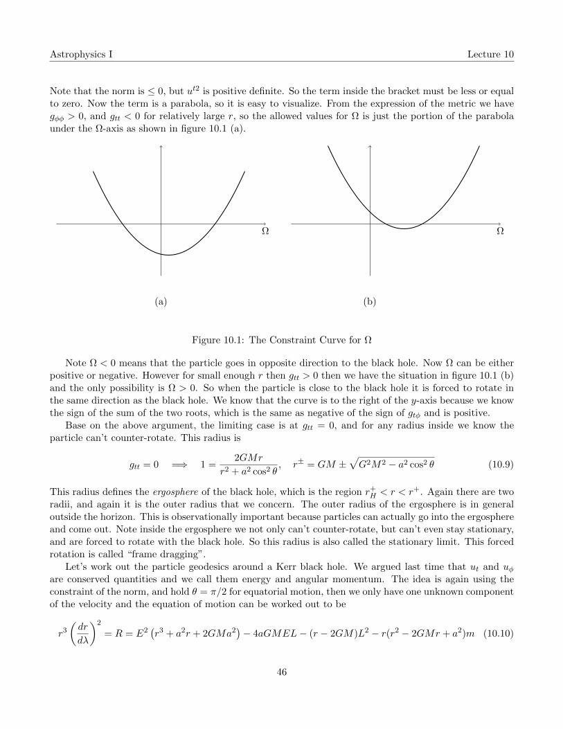
Astrophysics I Lecture 10
Note that the norm is ≤ 0, but ut2 is positive definite. So the term inside the bracket must be less or equalto zero. Now the term is a parabola, so it is easy to visualize. From the expression of the metric we havegφφ > 0, and gtt < 0 for relatively large r, so the allowed values for Ω is just the portion of the parabolaunder the Ω-axis as shown in figure 10.1 (a).
Ω
(a)
Ω
(b)
Figure 10.1: The Constraint Curve for Ω
Note Ω < 0 means that the particle goes in opposite direction to the black hole. Now Ω can be eitherpositive or negative. However for small enough r then gtt > 0 then we have the situation in figure 10.1 (b)and the only possibility is Ω > 0. So when the particle is close to the black hole it is forced to rotate inthe same direction as the black hole. We know that the curve is to the right of the y-axis because we knowthe sign of the sum of the two roots, which is the same as negative of the sign of gtφ and is positive.
Base on the above argument, the limiting case is at gtt = 0, and for any radius inside we know theparticle can’t counter-rotate. This radius is
gtt = 0 =⇒ 1 =2GMr
r2 + a2 cos2 θ, r± = GM ±
√G2M2 − a2 cos2 θ (10.9)
This radius defines the ergosphere of the black hole, which is the region r+H < r < r+. Again there are two
radii, and again it is the outer radius that we concern. The outer radius of the ergosphere is in generaloutside the horizon. This is observationally important because particles can actually go into the ergosphereand come out. Note inside the ergosphere we not only can’t counter-rotate, but can’t even stay stationary,and are forced to rotate with the black hole. So this radius is also called the stationary limit. This forcedrotation is called “frame dragging”.
Let’s work out the particle geodesics around a Kerr black hole. We argued last time that ut and uφare conserved quantities and we call them energy and angular momentum. The idea is again using theconstraint of the norm, and hold θ = π/2 for equatorial motion, then we only have one unknown componentof the velocity and the equation of motion can be worked out to be
r3
(dr
dλ
)2
= R = E2(r3 + a2r + 2GMa2
)− 4aGMEL− (r − 2GM)L2 − r(r2 − 2GMr + a2)m (10.10)
46
Astrophysics I Lecture 10
where m is 1 for massive particles and 0 for massless particles. It is a complicated equation but we caneasily check that under the limit a → 0 the equation reduces to the Schwarzschild case. Again we canfind the place of stable orbit by finding dR/dr = 0, and for circular orbits we even set R = 0. Withthese conditions we can completely solve the problem. We don’t want to write it down here but refer thereader to Schapiro and Teukolsky. In the end people are interested in the position of last stable orbits,and we quote the results here. For massless particles the last stable circular orbits are at GM and 4GMwhere at GM it is corotating. For massive particles it is at GM and 9GM with GM the corotating radiusand 9GM is the counter-rotating radius. The smallest corotating radius is inside the horizon, so it is notobservationally very relevant.
Let’s now do a thought experiment. It turns out that the ergosphere is more than a place where thereis no counter-rotation. In fact inside the ergosphere we can even have particles with negative energy. Let’stake the equation of motion (10.10) and solve for E, then we can write
E =2aGML+
(L2r2∆ +m2r∆ + r3
(drdλ
)2)1/2
r3 + a2r + 2Ma2(10.11)
For simplicity we consider photons m = 0 and we want to show that E < 0 is allowed. The inequality weneed is
L < 0, L2r2∆ + r3
(dr
dλ
)2
< 4a2G2M2L2 (10.12)
we can even eliminate the second term on the left if we only consider circular orbits. It turns out that thiscondition is actually equivalent to being inside the ergosphere. Penrose did a thought experiment aboutthis. Suppose we consider a particle coming into the ergosphere with some initial energy E. When it isinside the ergosphere it somehow decays into two particles, one of which having negative energy, which isallowed inside an ergosphere. Now suppose the negative energy particle gets captured into the horizon,but the positive energy particle escapes with energy E′. By energy conservation E′ > E and the particlegains energy by going through the ergosphere. This is called the Penrose process.
10.2 Accretion on the Black Hole
If a star forms a binary with a black hole, then when they rotate together the black hole will absorb matterfrom the star, and the matter will be accreted onto the black hole. We can work out the equipotentialsurfaces around the binary, and there is a crossing point between them, which is called the Lagrange point.If one of the stars is a red giant and the Lagrangian point will be contained inside the red giant and it willdonate mass to the other star. The region inside the equipotential surface connected to the Lagrange pointis called the Roche Lobe. This is believed how general accretion process works. However due to nonzeroangular momentum of the accretion matter they will not fall onto the other star immediately but will forman accretion disk. Due to viscosity and over time the matter will loose energy and start to fall into thestar, or black hole.
Let’s consider a star with an accretion disk around it. It can be a black hole, or a neutron star, oranything that can accrete. Why the matter always form a disk? The matter will scatter electromagneticradiation and loose energy in this way, so they will cool. But in this cooling there is no thermal supportin the direction parallel to the angular momentum, but angular momentum conservation prevents them tocollapse in the perpendicular direction, so in the end we will form a disk.
47

Astrophysics I Lecture 10
We can again use the Virial theorem and the energy per unit mass will be
E(r) =1
2v2 − GM
r= −1
2
GM
r(10.13)
Now in the accretion disk, due to viscosity the matter will loose angular momentum. Suppose material ofmass dm falls from r + dr to r, then the change of energy will be
dE
dm= −1
2
GM
r + dr+
1
2
GM
r=GM
2r2dr (10.14)
We are interested in the luminosity that we will get from an accretion of an annulus of width dr
dL =dE
dt=
1
2
GM
r2
dm
dtdr (10.15)
Note that dm/dt = −dM/dt is the rate at which the central star is gaining mass. This should be indepen-dent of r, otherwise we don’t have a constant process and there will be a radius at which the matter willfocus, instead of going into the central star. We want to convert the above expression to a temperatureprofile. The luminosity from an annulus is
dL = 2× 2πrσT 4 =1
2
GM
r2mdr (10.16)
Cancelling the dr on both sides we have
T =
(GMM
8πσ
)1/4
r−3/4 (10.17)
This is the temperature profile of an accretion disk. We can also work out the total luminosity
L =
∫dL =
1
2
∫GMM
r2dr =
1
2GMM
(1
rin− 1
rout
)∼ GMM
2rin(10.18)
where rin and rout are inner and outer radius of the accretion disk. In this way we can define some efficiency
η =L
Mc2=
1
2
GM
c2rin=
1/12, for rin = 6GM/c2
1/18, for rin = 9GM/c2
1/2, for rin ≈ GM/c2(10.19)
The first case is for Schwarzschild black hole, the second for counter-rotating orbits around maximallyrotating black holes, and the third one is for the corotating radius of the maximally rotating black holes.These numbers are to be contrasted with the efficiency of nuclear processes which are about η ≈ 0.07. Sothese will give much higher energy than the nuclear processes that fuel the stars, and this is why we get alarge luminosity increase near the center of a galaxy that a super-massive black hole situates.
48
Astrophysics I Lecture 11
11 Lecture 11
11.1 Generation of Gravitational Waves
From today we will start to talk about gravitational waves. A good reference is the chapter 7 of Carroll.Let’s recall a simpler example which is electromagnetic waves. Recall half of the the Maxwell equations
∂νFνµ = −Jµ, where Fµν = ∂µAν − ∂νAµ (11.1)
If we plug in the expression of Fµν in terms of Aµ, then we will get an equation for Aµ
∂ν (∂νAµ − ∂µAν) = Aµ − ∂µ∂ ·A = −Jµ (11.2)
The other half of the Maxwell equations is automatically satisfied by the definition of Fµν :
∂νFνµ = 0 (11.3)
Now if we look at the equation (11.2), and choose the Lorentz gauge ∂νAµ = 0 then the second term
on the left vanishes, and we have a wave equation with source
Aµ = −Jµ (11.4)
From here on it is easy to solve the equation and obtain the wave solution. Now a question is whether wecan always choose the Lorentz gauge ∂µA
µ = 0. Note Fµν is gauge invariant by its definition, so we wantto find a gauge transformation Aµ → Aµ + ∂µΛ such that the resulting Aµ satisfies the gauge condition.We want
∂µA′µ = ∂µ(Aµ + ∂µΛ) = 0 =⇒ Λ = −∂µAµ (11.5)
Now this Λ can always be found because this is just another wave equation with source. Therefore theLorentz gauge can always be attained.
Let’s now come to GR. The equation now is
Gµν = Rµν −1
2Rgµν = 8πGTµν (11.6)
Here the equation is more complicated than Maxwell equations in that it is nonlinear. However in mostcases we are interested in, the gravitational wave is weak, and we expand the metric around Minkowski
gµν = ηµν + hµν (11.7)
Now we can plug this into the Einstein equations and obtain an equation for the perturbation hµν . Theleft hand side is
Gµν = Rµν −1
2gµνR = −1
2
[hµν − ηµνh+ ∂µ∂νh+ ηµν∂α∂βh
αβ − ∂µ∂βhβν − ∂ν∂βhβµ
](11.8)
This looks like a mess. Similar to the Maxwell case, we can simplify the equation by choosing a gauge.The gauge transformations in GR is actually changing frames, changing xµ → x′µ. The transformation ofthe metric is
g′µν(x′) = gαβ(x)∂xα
∂x′µ∂xβ
∂x′ν(11.9)
49
Astrophysics I Lecture 11
Suppose we write the transformation in a specific way xµ → xµ − ξµ. Then we can write the gaugetransformation on the metric as
g′µν(x′) = gαβ(x′ + ξ)∂(x′α + ξα)
∂x′µ∂(x′β + ξβ)
∂x′ν(11.10)
In the case where ξµ is small, we can expand the whole equation and we get
ηµν + h′µν = (ηµν + hµν)(δαµ + ∂µξ
α) (δβν + ∂νξ
β)
= ηµν + hµν + ∂µξν + ∂νξµ(11.11)
where we have thrown away higher order terms. This is the gauge transformation for the metric pertur-bation. The choice of ξµ is entirely arbitrary, so we can choose gauges that enable us to see things moreclearly.
The first gauge choice we shall make is the transverse traceless gauge. By this we mean
hii = 0, ∂ihij = 0 (11.12)
where indices run over space but not time. This choice can be done when Tµν = 0. Let’s look at the 00component of Einstein equations in this gauge
h00 −h00 + ∂20(−h00)−
(∂2
0h00 + 2∂0∂ih
0i)− 2∂2
0h00 − 2∂0∂ih
i0 = 0 (11.13)
We can raise some indices and we can find the left hand side always cancel, and the result is consistent withTµν = 0. In fact if Tµν 6= 0 then this gauge is inconsistent. Similarly we can work out the 0i componentand we will find the equation reduces to
∇2h0i − ∂i∂jhj0 = 0 (11.14)
Note that our gauge choice does not completely fix the gauge, and we can in addition demand that∂jh
j0 = 0. Then we will get ∇2h0i = 0 and if we assume h vanish at infinity then h0i = 0 identically.
Let’s now look at the ij component of the equation. We have
hij + δijh00 + ∂i∂j(−h00) + δij
(∂2
0h00 + 2∂0∂kh
0k)− ∂i∂0h
0j − ∂j∂0h
0i = 0 (11.15)
We can again impose ∂jhj0 = 0, then we get
hij + δij∇2h00 − ∂i∂jh00 = 0 (11.16)
If we take trace on the whole equation we can get 2∇2h00 = 0 and again from boundary condition we canget h00 = 0. So the above equation reduces to
hij = 0 (11.17)
This is just a freely propagating wave. Now the matrix hij has 6 components because it is a 3 × 3 sym-metric matrix, but we need to subtract the 4 gauge conditions, and there are only 2 physical polarizationsremaining. Therefore it turns out that there are only two polarizations for gravitational waves, just as forelectromagnetic waves.
50
Astrophysics I Lecture 11
Let’s try to solve the wave equation. We can take an ansatz
hij = cijeik·x =⇒ −k2cij = 0, k2 = 0 (11.18)
Therefore the wave is propagating at the speed of light, which can also be seen from the fact that there is nomass term in the wave equation. Now from the gauge conditions we can get constraints on the coefficientcij . The traceless condition tells us that cii = 0. The transverse condition gives us
∂ihij = 0 =⇒ kicij = 0 (11.19)
Let’s assume without loss of generality that kµ is along the z-direction and that kµ = (1, 0, 0, 1). Then cijmust be written in the following matrix form
cij =
h+ h× 0h× −h+ 00 0 0
(11.20)
So the matrix is parametrized by two parameters only, and they are the amplitudes of two polarizations.So we can write the wave solution as
hij = eik·x
h+
1 0 00 −1 00 0 0
+ h×
0 1 01 0 00 0 0
(11.21)
These two polarizations are analogue to the two polarizations of the electromagnetic wave.Now let’s consider another gauge choice which is called the harmonic gauge. The condition is
∂µhµν −1
2∂νh = 0 (11.22)
This is a close analogue to the Lorentz gauge in electromagnetism, and it is also called the Lorenz gauge,or de Donder gauge. Let’s show that this gauge choice can always be made. Let h′µν = hµν + ∂µξν + ∂νξµ,then
∂µh′µν −1
2∂νh
′ = ∂µhµν −1
2∂νh+ξν −
1
2∂ν∂µξ
µ + ∂ν∂µξµ − 1
2∂ν∂µξ
µ (11.23)
So in order to satisfy the gauge condition we only need to choose
ξν = −(∂µhµν −
1
2∂νh
)(11.24)
which is just a wave equation with some source. Therefore this is a more general gauge than the previoustransverse traceless gauge. Now let’s substitute the gauge condition into our linearized Einstein equation,and we will get
hµν −1
2ηµνh = −16πGTµν , or hµν = −16πG
(Tµν −
1
2ηµνT
)(11.25)
This equation is convenient for our purpose because we want to study how gravitational wave is generatedby binary orbiting objects. We can define a more convenient quantity hµν as
hµν = hµν −1
2ηµνh =⇒ h = −h (11.26)
51

Astrophysics I Lecture 11
Therefore the linearized Einstein equation looks like
hµν = −16πGTµν (11.27)
We can solve this equation by means of Green functions. We introduce G(x−y) such that G(x−y) =δ4(x− y). Then we can formally write the solution as
hµν(x) = −16πG
∫d4y Tµν(y)G(x− y) (11.28)
Recall the Green function for the wave equation is just
G(x− y) = − 1
4π |x− y|δ(|x− y| −
∣∣x0 − y0∣∣) θ(x0 − y0) (11.29)
This is the retarded Green function where causality is enforced. If we plug this into the formal integral wewill get
hµν(x, t) = 4G
∫d3y
1
|x− y|Tµν(tR,y) (11.30)
where tR = t− |x− y| is the retarded time. This is the form of solution that we will be working with. Itis more convenient to work in the Fourier space
˜hµν(ω,x) =1√2π
∫dt hµν(x, t)eiωt
=4G√2π
∫dt d3y eiωt
Tµν(tR,y)
|x− y|
=4G√2π
∫dtR d
3y eiωtReiω|x−y|Tµν(tR,y)
|x− y|
(11.31)
Now the integration on tR is just the Fourier transform of Tµν , so we have
˜hµν(ω,x) = 4G
∫d3y eiω|x−y|
Tµν(ω,y)
|x− y|(11.32)
So far we haven’t introduced any approximations. Now let’s assume that we are very far away comparedto the region emitting the gravitational wave, or where Tµν 6= 0, then
eiω|x−y|
|x− y|∼ eiωr
r(11.33)
where r = |x|. Therefore we have
˜hµν(ω,x) ∼ 4Geiωr
r
∫d3y Tµν(ω,y) (11.34)
In fact the only components that we need to figure out are ˜hij , and the other components follow from theharmonic gauge condition
iω˜h0ν = ∂i˜hiν (11.35)
52

Astrophysics I Lecture 11
We can write the integrand which is Tij in the following useful form∫d3y Tij(ω,y) =
∫d3y
[∂k
(yiTkj
)− yi∂kTkj
](11.36)
The first term on the right vanishes if the source is localized. The second term can be simplified using theconservation of energy momentum ∂µT
µν = 0, so that
− iωT 0j + ∂iTij = 0 (11.37)
Plug this into our formal solution we have
˜hij(ω,x) = iω4Geiωr
r
∫d3y yiT0j (11.38)
We can do this trick again to pull another y in front of T , so that we will have
˜hij(ω,x) = −2Gω2eiωr
r
∫d3y yiyj T
00(ω,y) (11.39)
This is the quadrupole formula because T 00 is the energy density and we are integrating over the quadrupolemoment. The integral is usually written as Iij(ω). If we take a Fourier transform back to position spacethen we will get
hij(t,x) =2G
r
d2
dt2RIij(tR), where Iij(tR) =
∫d3y yiyjT
00(tR,y) (11.40)
53

Astrophysics I Lecture 12
12 Lecture 12
Last time we calculated the gravitational quadrupole radiation produced by some energy density
˜hij(ω,x) = −2Gω2eiωr
r
∫d3y yiyj T
00(ω,y) = −2Gω2eiωr
rIij(ω) (12.1)
where we have taken the Harmonic gauge condition
∂µhµν −1
2∂νh = ∂µhµν = 0 (12.2)
An inverse Fourier transform will give us
hij(t,x) =2G
r
d2
dt2RIij(tR), where Iij(tR) =
∫d3y yiyjT
00(tR,y) (12.3)
where recall that tR is the retarded time tR = t− |x− y|. The fact that gravitational waves are generatedby quadrupoles means that a perfectly spherical symmetric body will not generate any gravitational wave.
12.1 Calculation of Gravitational Wave Production
Today we want to do some things with the above formula, and calculate the actual wave produced by somesystems. We will also try to work out the energy loss by radiation of gravitational waves. Let’s considera system with two stars going around each other, and we want to calculate the quadrupole of this pairof binaries. We can treat the orbit of the binary using Newtonian mechanics, under the assumption thattheir separation is not so small. Let’s also assume that the two masses are the same M with a perfectcircular orbit with radius R. The force on one of the stars due to the other star is
F =GM2
(2R)2=Mv2
R=⇒ v =
√GM
4R(12.4)
For our purpose it is more convenient to consider the angular frequency
T =2πR
v=⇒ Ω =
2π
T=
√GM
4R3(12.5)
We will approximate the two stars as point masses, and their energy (or mass) densities are just deltafunctions. The positions of the two stars are
ya1 = R cos Ωt
ya2 = R sin Ωtand
yb1 = −R cos Ωt
yb2 = −R sin Ωt(12.6)
Using these information we can write our energy density as
T 00(t,y) = Mδ(y3)[δ(y1 − ya1)δ(y2 − ya2) + δ(y1 − yb1)δ(y2 − yb2)
](12.7)
Now we can plug in the formula for Iij and calculate the quadrupole moment
Iij = MR2
(1 + cos 2Ωt) sin 2Ωt 0sin 2Ωt (1− cos 2Ωt) 0
0 0 0
(12.8)
54

Astrophysics I Lecture 12
We can take time derivatives on the quantities directly and we will get the answer for gravitational waves
hij(t,x) =2GMR2
r(−4Ω2)
cos 2ΩtR sin 2ΩtR 0sin 2ΩtR − cos 2ΩtR 0
0 0 0
= − R2s
2rR
cos 2ΩtR sin 2ΩtR 0sin 2ΩtR − cos 2ΩtR 0
0 0 0
(12.9)
where Rs = 2GM is the Schwarzschild radius.Let’s plug in some numbers. Assume M ∼ 10M, and the Schwarzschild radius is about 106 cm. Let’s
assume that R ∼ 107 cm, which is about 10 times the Schwarzschild radius. The frequency will then be
f =Ω
2π∼ 102 Hz (12.10)
This is the typical gravitational wave frequency, and it is the frequency LIGO is trying to observe. Nowthe more interesting thing is to calculate the magnitude of hij . A reasonable distance r could be estimatedusing the probability of this kind of event to occur in the universe. The LIGO expects the distance to beabout r ∼ 100 Mpc ∼ 1026 cm. So we can estimate
∣∣hij∣∣ ∼ R2s
2rR∼ 10−21 (12.11)
So the distance fluctuation that LIGO is trying to detect is 1 km, which is the arm length, times the abovequantity, and that is 10−15 cm.
12.2 Energy of Graviton
Let’s try to understand the energy carried by gravitons in the form of gravitational waves. Remember ourway of approaching the gravitational wave problem was to expand the metric around flat metric and keptthe first order in perturbation. However as Einstein’s equations are highly nonlinear, we can break theEinstein tensor into different orders of hµν
Gµν = G(1)µν +G(2)
µν + . . . (12.12)
where G(1)µν is the first order correction due to h and we worked it out to be
G(1)µν = −1
2hµν (12.13)
Now formally we can keep only this term on the left side, and move all the higher order terms to the righthand side
G(1)µν = 8πG
(Tµν −
G(2)µν
8πG+ . . .
)= 8πGtµν (12.14)
where we call tµν the “pseudo-energy-momentum” tensor. It is not a tensor because we only kept part ofthe tensor Gµν . If we want to use this as a good energy-momentum tensor, we need it to be symmetric,but also conserved. It is obviously symmetric because it is constructed from Tµν and parts of Gµν . As forconservation, in fact it is not conserved covariantly, but we claim that
∂µtµν =1
8πG∂µG(1)
µν = 0 (12.15)
55
Astrophysics I Lecture 12
This can be directly checked using the expression for G(1)µν
∂µG(1)µν =
(∂µhµν −
1
2∂νh
)= 0 (12.16)
Now that we have identified the “pseudo” energy-momentum tensor for the metric perturbation, wecan calculate the amount of energy that is carried away by the gravitational wave. Our goal is to obtain aradiative power of the gravitational radiation. Now we need to calculate the second order Einstein tensor
R(2)µν =
1
2hρσ∂µ∂νhρσ +
1
4(∂µhρσ)∂νh
ρσ + (∂σhρν)∂[σhρ]µ − hρσ∂ρ∂(µhν)σ
+1
2∂σ(hρσ∂ρhµν)− 1
4(∂ρhµν)∂ρh− (∂σh
ρσ − 1
2∂ρh)∂[µhν]ρ
(12.17)
This is a messy expression! If we choose the Harmonic gauge then the expression can be largely simplified⟨R(2)µν
⟩= −1
4
[∂µh
ρσ∂νhρσ −1
2∂µh∂νh
](12.18)
Note the angular bracket around R(2)µν . This is because we expect the energy momentum tensor to occur
under an integral, so we can do integration by parts on the expression
〈A∂µB〉 = −〈B∂µA〉 (12.19)
Not that we are actually doing any integration here, but we anticipate that the quantity of interest will beintegrated over space and time. The integration over time is an average over many cycles, which we willalso do if we want to get an average power output. This gives us great simplification in the expression, ascan be seen above. If we take trace on the above expression we will get 0 if we use the Harmonic gaugecondition.
With this tensor, we can now write down the energy-momentum tensor of the graviton
tgravµν = − 1
8πGG(2)µν (12.20)
So we have⟨tgravµν
⟩=
1
32πG
(∂µh
ρσ∂νhρσ −1
2∂µh∂νh
)=
1
32πG
(∂µh
ρσ∂ν hρσ −1
2∂µh∂ν h
)(12.21)
Now before we could plug into the above equation, we need to work out h0i and h00 from hij which wesolved a while ago. We do this by using the Harmonic gauge condition ∂µhµν = 0:
∂0h00 + ∂ih0i = 0, ∂0h0j + ∂ihij = 0 (12.22)
The second equation gives us
∂th0j = ∂ihij = ∂i(
2G
r
d2
dt2RIij
)(12.23)
The derivative acts on both terms in the bracket, but we argue that the derivative acting on 1/r will giveus 1/r2 which decays faster than the other term, so we can safely keep only the second term
∂th0j ∼ −2G
rni
...I ij =⇒ h0j = −2G
rniIij (12.24)
56
Astrophysics I Lecture 12
where we have written tR = t − n · x, and n is the direction that points from the source to the observer.Now we only need to evaluate h00 similar as above so we will get
h00 =2G
rninj Iij (12.25)
Now remember that in the energy-momentum tensor, the components t0i are the energy flux along thei direction. So in order to get the total power we should take this vector dotted wiht ni and integrate itover a total area at some distance r away.
P =
∫t0in
ir2 dΩ (12.26)
Whereas the power radiated into a direction is just
dP
dΩ= t0in
i = − G8π〈...I ij
...I pq〉
[δipδjq − 2ninpδjq +
1
2ninjnpnq − 1
2δijδpq +
1
2ninjδpq +
1
2δijnpnq
](12.27)
Let’s plug in the physical situation of the binary star and we will get
dP
dΩ= −16
πGM2R4ω6
[1− sin2 θ +
1
8sin4 θ
](12.28)
The power is negative because the convention is that we are calculating the energy change of the binarysystem, and it is obviously emitting gravitational wave, so the energy is decreasing.
57

Astrophysics I Lecture 13
13 Lecture 13
13.1 Gravitational Wave Braking
Remember last time we calculated the gravitational wave production of an equal-mass binary system. Thepower output, or energy change of the system was worked out as
dP
dΩ= −16
πGM2R4ω6
[1− sin2 θ +
1
8sin4 θ
](13.1)
where ω is the angular frequency that the binary go around each other. Today we can apply this formulato actual physical systems. In order to do that we integrate this formula over all solid angle
P =
∫dP
dΩdΩ = −128
5GM2R4ω6 = −2
5
G4M5
R5=dE
dt(13.2)
This is the total power emitted from the binary system. The total energy of the system can be found bythe summing the kinetic energy of the two stars and the gravitational potential energy between the stars
E = Mv2 − GM2
2R= −GM
2
4R(13.3)
Once we have this we can plug this into the power equation to get the change of orbital radius with respectto time
− GM2
4R2
dR
dt=
2
5
G4M5
R5=⇒ dR
dt= −8
5
G3M3
R3(13.4)
Therefore because of the gravitational wave radiation the orbit of the binary will slowly decay. Let’s tryto evaluate this in the earth-sun system, assuming that the earth has the same mass as the sun. In fact inthis system we have GM/R ∼ 10−8, so the fractional change of R in unit time interval will be
1
R
dR
dt∼ 10−24 c
R≈ 10−25 min−1 (13.5)
This is an incredibly small fraction of orbital radius that the change can never be detected using ourexperimental equipments. However there are systems out there in the universe that we can observe thisslow down effect. A well known example is the PSR B1913+16 pulsar. The observed cumulative periodshift of the binary matches exactly the predictions of general relativity, which is just our above formula.This is a beautiful confirmation of the existence of gravitational waves.
The LIGO experiment is an effort to detect gravitational waves. The structure is similar to that ofMichelson-Morley experiment with two arms of approximately 1 km with light beams bouncing aroundaround 100 times in each arm and brought back together to interfere. We can do a rough estimate of themaximum and minimum frequency that this apparatus can detect. Because light takes time to go aroundthe 100 km arm length, the maximum frequency that it can detect should be about 103 Hz. Because ofthe finite span of the project, the lowers frequency that it can detect should be approximately 10−7 Hz.However due to seismic activity and other constraints, LIGO can’t really get precise measurements forwaves at such low frequency. In fact its optimal frequency range is actually from 10 Hz to 104 Hz. Thebest sensitivity is at about 100 Hz. The sensitivity is plotted below in figure 13.1.
58
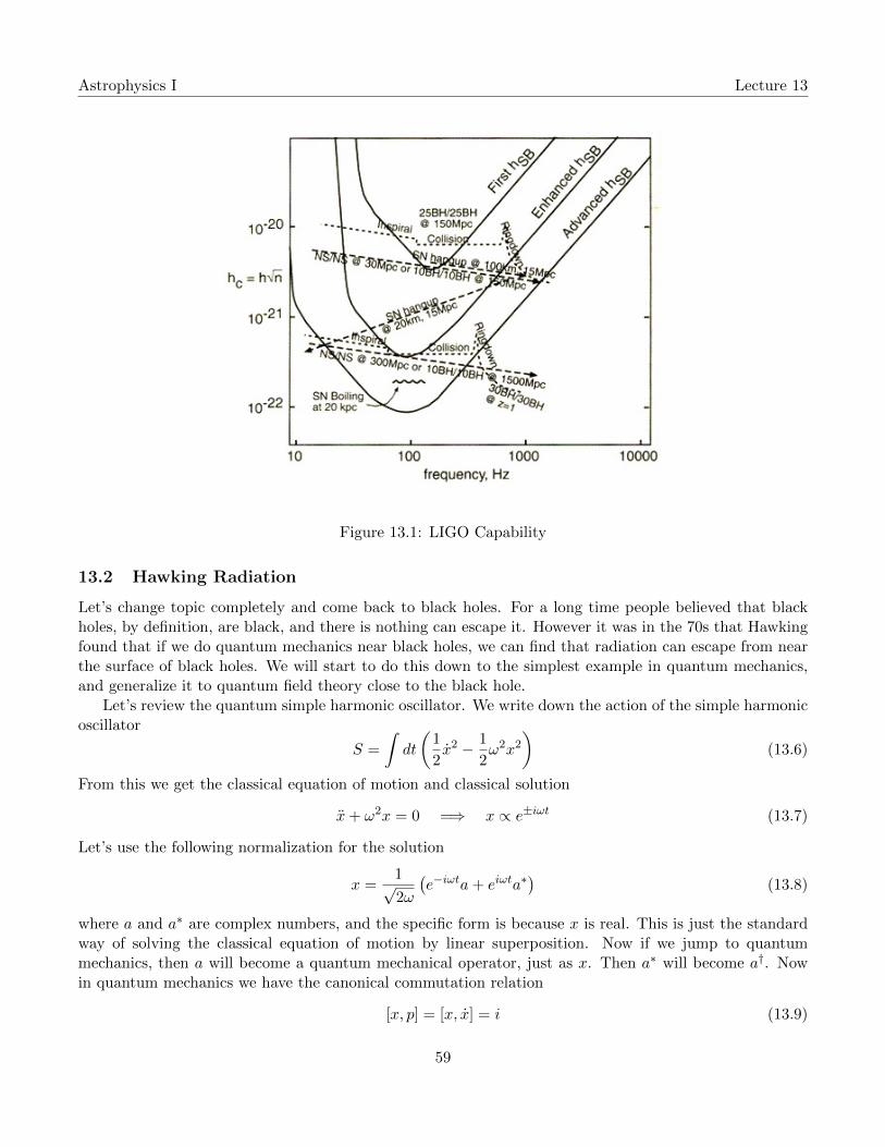
Astrophysics I Lecture 13
Figure 13.1: LIGO Capability
13.2 Hawking Radiation
Let’s change topic completely and come back to black holes. For a long time people believed that blackholes, by definition, are black, and there is nothing can escape it. However it was in the 70s that Hawkingfound that if we do quantum mechanics near black holes, we can find that radiation can escape from nearthe surface of black holes. We will start to do this down to the simplest example in quantum mechanics,and generalize it to quantum field theory close to the black hole.
Let’s review the quantum simple harmonic oscillator. We write down the action of the simple harmonicoscillator
S =
∫dt
(1
2x2 − 1
2ω2x2
)(13.6)
From this we get the classical equation of motion and classical solution
x+ ω2x = 0 =⇒ x ∝ e±iωt (13.7)
Let’s use the following normalization for the solution
x =1√2ω
(e−iωta+ eiωta∗
)(13.8)
where a and a∗ are complex numbers, and the specific form is because x is real. This is just the standardway of solving the classical equation of motion by linear superposition. Now if we jump to quantummechanics, then a will become a quantum mechanical operator, just as x. Then a∗ will become a†. Nowin quantum mechanics we have the canonical commutation relation
[x, p] = [x, x] = i (13.9)
59
Astrophysics I Lecture 13
We can plug the above expression for x into the above commutation relation and get a commutationrelation of the a and a† operators
[a, a†] = 1 (13.10)
We know that a and a† are ladder operators for the simple harmonic oscillator states, and they relate theenergy eigenstates to one another. If we call |0〉 the ground state, then a† |0〉 is the first excited state,a†a† |0〉 proportional to the second excited state, etc. Remember the Hamiltonian will be diagonalized as
H =
(a†a+
1
2
)ω, En =
(n+
1
2
)ω (13.11)
The crucial thing here is again the commutation relation between a and a†.Now we will do Hawking radiation in this language. Essentially what happens is that the black hole
gives the frequency a time dependency and this will change the ground state into excited states due tothis time dependence of frequency. However we will not do it in that way. We will add a time-dependent“electric field” to the action
S =
∫dt
(1
2x2 − 1
2ωx2 + Ex
)(13.12)
Then the classical equation of motion will become
x+ ω2x = E (13.13)
We will consider a time dependent E(t) which is 0 in the far past, and is E0 in the far future, and it isgradually turned on around t ∼ 0. In the far past we have already solved like above. In the far futurewhen E = E0 we need to do this again. Because of the simplicity of the problem we can actually solve itanalytically. We can redefine y = x− E0/ω
2 and the equation of motion will become
y + ω2y = 0 (13.14)
so we recover another simple harmonic oscillator in y. This is because E0 is a constant and time derivativedoes not act on it. So we can write the solution as
y =1√2ω
(e−iωtb+ eiωtb†
)=⇒ x =
E0
ω2+
1√2ωe−iωtb+
1√2ωeiωtb† (13.15)
Let’s consider the extreme limit that the electric field is turned on suddenly, such that E = E0θ(t).Now what we want to do is to match the two solution at far past and far future at the point t = 0, requiringthat x and x to be continuous at t = 0. The continuity of x will tell us that
E0
ω2+
1√2ωb+
1√2ωb† =
1√2ωa+
1√2ωa† (13.16)
whereas continuity of x will tell us thata† − a = b† − b (13.17)
These two equations will tell us that a and b are related by
b = a− E0
ω√
2ω, b† = a† − E0
ω√
2ω(13.18)
60

Astrophysics I Lecture 13
This is actually Hawking radiation in disguise. Suppose the system is in the ground state |0〉 at t < 0. Butnow what ground state are we in, as there are now two annihilation operators? Let’s suppose the system isoriginally in |0〉a, which means that a |0〉a = 0, then after we turn on the electric field the notion of groundand excited state changes. Now we have
b†b |0〉a =
(a† − E0
ω√
2ω
)(a− E0
ω√
2ω
)|0〉a = − E0
ω√
2ω|1〉a +
E20
2ω3|0〉a (13.19)
Now if we calculate the expectation of particle number nb = b†b then we get⟨0∣∣∣b†b∣∣∣ 0⟩
a a=
E20
2ω3(13.20)
Therefore there will be particles in the new spectrum in the presence of electric field. So when we go fromthe situation without electric field to the situation with electric field, we are changing the definition of whatis vacuum and what is particle, and this in effect gives us extra particles from nothing. This means thatthe vacuum for one observer will be populated by particles for another observer, and this is the essence ofHawking radiation.
What happens in Hawking radiation is that when we have a black hole in the background, the definitionof vacuum becomes ambiguous. The gravitational field will replace the electric field above, and its presencewill change the spectrum of the system just like the electric does.
We can solve the above problem for any function E(t) using the means of Green functions. In fact ifE(t) is turned on adiabatically, or very slowly, then we will find that the vacuum structure will not bechanged, and there is no particle creation. In this sense “speed” of turning is crucial in this effect, so thisis why we need a black hole in the background to produce Hawking radiation, where gravitational fieldchanges dramatically in very small distances.
13.3 Crush Course on Quantum Field Theory
Now let’s come to field theory and generalize our toy model above. Consider a massless scalar field φ(t, x).The action is now
S =
∫dt dx
(1
2(∂tφ)2 − 1
2(∂xφ)2
)(13.21)
The classical equation of motion will be the massless Klein-Gordon equation
φ = −∂2t φ+ ∂2
xφ = 0 (13.22)
If we do a Fourier transformation into k space like
φ(t, x) =1√2π
∫dk φ(t, k)eikx (13.23)
then our equation will be reduced to exactly the same as the quantum harmonic oscillator equation
¨φ+ k2φ = 0 (13.24)
However the difference from the harmonic oscillator case is that we actually have an infinite number ofharmonic oscillators labelled by the wave number k. The dispersion relation in this massless case is justω = |k|. So we can write the solutions as
φ(t, x) =
∫dk√2π
1√2ω
(e−iωt+ikxak + eiωt−ikxa†k
)(13.25)
61

Astrophysics I Lecture 13
which is just like the harmonic oscillator case, except that we have an integration over k. Here a†k and akare creation and annihilation operators that create and annihilate particles with momentum k. So a†k |0〉will be a state with one free massless scalar particle with momentum k. The analogue of the momentumoperator is π = φ, and the analogue of the canonical commutation relation is
[φ(t, x), π(t, y)] = iδ(x− y) (13.26)
The analogue of the commutation relations between a and a† is just
[ak, a†k′ ] = 2πδ(k − k′) (13.27)
62

Astrophysics I Lecture 14
14 Lecture 14
Today is our last lecture. We want to start by recalling something from the last lecture. We considered asimple harmonic oscillator with a time-dependent external electric field. The electric field was turned onat some time, and we found that the vacuum and excited states are different in different electric fields. Soif we start with the vacuum state of E = 0, when the electric field is turned on the state will no longer bethe vacuum in the new spectrum with the background field. We found that⟨
0∣∣∣b†b∣∣∣ 0⟩
a 0=
E2
2ω36= 0 (14.1)
The mismatch of spectrum is due to the background electric field. In the case of Hawking radiation, themismatch is between a free-falling observer outside a black hole, and an observer located on the horizon.In the vacuum state with respect to the free-falling observer, the observer at the event horizon will seeexcitations which are the origin of the Hawking radiation.
Let us consider things in 2 dimensions, namely r and t, in order to make things simpler. TheSchwarzschild metric is
ds2 = −(
1− 2GM
r
)dt2 +
(1− 2GM
r
)−1
dr2 =
(1− 2GM
r
)[−dt2 + dr2
∗]
(14.2)
where we define r∗ as
r∗ = r + 2GM ln( r
2GM− 1)
(14.3)
Recall our discussion about the singularity at r = 2GM , which is just an artifact of the coordinate choice.We can remove the singularity by going to the Kruskal coordinates
ds2 =2GM
re−r/2GM
[−dT 2 + dR2
](14.4)
where we defined
T = a−1ear∗ sinh(at), R = a−1ear∗ cosh(at), a =1
4GM(14.5)
It is straightforward to check that this coordinate transformation will yield the above metric in equation(14.4). Note that in the above definition of r∗ the horizon actually corresponds to r∗ = −∞ and there is nodefinition of r∗ inside the event horizon. If we want to go across the horizon then we need to analyticallycontinue r∗ into r < 2GM region. In fact that is precisely what we want to do, and we are going to go tothe part R < 0 by analytic continuation. So it is more convenient to consider the above metric defined onthe whole spacetime for any T and R. Now our above definition of R is manifestly positive, so when weanalytically continue it to region II in diagram 14.1 we pick up a minus sign, and so does T . We will usethe following expressions for T and R in region II
T = −a−1ear∗ sinh(at), R = −a−1ear∗ cosh(at) (14.6)
Note that both regions I and II are the exterior of the black hole, however they can never communicate,and when we interpret region I as our physical world we can think of region II as another world whichis disconnected from ours. What we will do next is to express the creation and annihilation operators interms of the two different coordinates (or observers). In particular we will take the frame of an observer
63

Astrophysics I Lecture 14
R
T r∗ → −∞, T = R, t→∞
r∗ → −∞, T = −R, t→ −∞
r∗ = const
t = const
r = 0
Region IRegion II
Figure 14.1: Spacetime Diagram for Black Hole
at constant r∗, which is an observer at the horizon, and another at constant R, which approximatelycorresponds to a free-falling observer.
The field we are going to consider is the free massless scalar field with classical equation of motion
φ =(−∂2
t + ∂2r
)φ = 0 (14.7)
Let’s try to solve the classical equation of motion in the curved coordinates. Now we need to ask ourselveswhat is φ in curved space? A useful formula that we will use is
φ =1√−g
∂µ(gµν√−g∂νφ
)(14.8)
which is just a special case of the following formula in GR
∇µvµ =1√−g
∂µ(√−gvµ
)(14.9)
We first do it in the extended Kruskal coordinates. This form of the equation is very useful in our casebecause we can easily evaluate
√−g which is just our conformal factor
√−g =
2GM
re−r/2GM (14.10)
and this cancels the factor gµν in front, so we recover exactly the same equation as in flat space
φ =1√−g(−∂2
T + ∂2R
)φ = 0 (14.11)
and we know the solution as a linear combination of plane waves
φ(T,R) =
∫dk√2π
1√2ω
(e−iωT+ikRak + eiωT−ikRa†k
)(14.12)
64

Astrophysics I Lecture 14
Now we can repeat the above steps for the original Schwarzschild metric. It seems that the same waveequation is going to hold, and the logic seems to follow in the same way and we should have the samesolution. But this is not what we want, and there has to be some caveat somewhere. However let’s justwrite down the equation and solution(
−∂2t + ∂2
r∗
)φ = 0, φ(t, r∗) =
∫dk√2π
1√2ω
(e−iωt+ikr∗bk + eiωt−ikr∗b†k
)(14.13)
We claim that this solution is incomplete. This is because the coordinate we have here does not cover thewhole space. Note our definition of T , and it is obvious that in region II T will have a different sign fromt, and in this region T and t will flow in different directions. Now if T is the correct sense of time, thenthe positive frequency mode in region I will turn out to be negative frequency modes in region II. In orderto resolve this, we define two sets of mode functions, in region I and II respectively
g(1)k =
1√
(2π)(2ω)e−iωt+ikr∗ in region I
0 in region II
, g(2)k =
0 in region I1√
(2π)(2ω)e+iωt+ikr∗ in region II
(14.14)
Now these are the correct positive frequency modes in the corresponding region in spacetime, and thesolution should be written as
φ(t, r∗) =
∫dk b
(1)k g
(1)k + b
(1)†k g
(1)∗k + b
(2)k g
(2)k + b
(2)†k g
(2)∗k (14.15)
In principle we can now compare our two solutions and express b(1)k and b
(2)k in terms of ak and a†k. Then
we can compute particle creation by working out the expectation value of one particle with respect to theother vacuum. However this is a messy route, and we want to do something a little different.
The trick we are going to use involves rewriting the mode functions a bit. In stead of figuring outdirectly the relations between ak and bk, we introduce a set of operators ck and c†k. The important featureis that it turns out that ck annihilates the same vacuum as ak, and the relation between ck and bk is easierto find. So we just need to find out the vacuum in terms of ck operators and find the expectation values
of b†kbk in this vacuum. Let’s try to write the mode functions g(1)k in region I in terms of the Kruskal
coordinates√
4πωg(1)k = e−iω(t−r∗) =
(e−at+ar∗
)iω/a= (aR− aT )iω/a
(14.16)
Now expressed in terms of the global coordinates R and T this expression is meaningful not only in regionI, but also in region II. In fact if we consider the same thing in region II we have
√4πωg
(2)∗−k = e−iω(t−r∗) =
(e−at+ar∗
)iω/a= (aT − aR)iω/a = (e−iπ)iω/a (aR− aT )iω/a
= eπω/a (aR− aT )iω/a
(14.17)
Now we know that the quantity (aR − aT )iω/a is defined in both region I and II, and it can in fact bewritten as
aiω/a(R− T )iω/a =√
4πω(g
(1)k + e−πω/ag
(2)∗−k
)(14.18)
65
Astrophysics I Lecture 14
Note the imaginary power should be understood as the following
(R− T )iω/a = exp
[iω
aln(R− T )
]= exp
[iω
aln |R− T |+ ω
aarg(T −R)
](14.19)
The branch cut is chosen such that when arg(T − R) is negative the above function is analytic, whichcorresponds to the positive frequency modes because the mode functions e−iω(T−R) for positive frequencyhas the same analytic behavior, i.e. analytic in the lower half of the complex plane of R−T . So this meansthat the above function contains only the positive frequency mode in the T,R version of the field φ. Sothese are as good a set of mode functions as our original set e±iω(T−R). Let’s write down the new modefunctions
h(1)k =
1√2 sinh(πω/a)
(eπω/2ag
(1)k + e−πω/2ag
(2)∗−k
)(14.20)
h(2)k =
1√2 sinh(πω/a)
(eπω/2ag
(2)k + e−πω/2ag
(1)∗−k
)(14.21)
These hk functions are properly orthonormal in the following norm
(fk1 , fk2) = −i∫dR
(fk1∂T f
∗k2 − f
∗k2∂T fk1
)(14.22)
Now if we use these as mode functions we can rewrite our mode expansion of the scalar field as
φ(t, r∗) =
∫dk(c
(1)k h
(1)k + c
(1)†k h
(1)∗k + c
(2)k h
(2)k + c
(2)†k h
(2)∗k
)(14.23)
Because we have shown that h(1)k are those positive frequency modes in the Kruskal frame, so we should
expect ck |0〉a = 0. However we claim and will show that bk |0〉a 6= 0. We can see this by matchingcoefficients between the two different expressions of φ(t, r∗) and get
b(1)k =
1√2 sinh(πω/a)
(eπω/2ac
(1)k + e−πω/2ac
(2)†−k
)(14.24)
b(2)k =
1√2 sinh(πω/a)
(eπω/2ac
(2)k + e−πω/2ac
(1)†−k
)(14.25)
Now we are ready to write down the famous Hawking formula by evaluating the expectation value of
number of b(1)k particles in the a-vacuum, or equivalently the c-vacuum.⟨
0∣∣∣b(1)†k b
(1)k
∣∣∣ 0⟩c c
=1
2 sinh(πω/a)e−πω/aδ(0) (14.26)
The coefficient in front of the delta function can be written in the more familiar form
1
2 sinh(πω/a)e−πω/a =
1
e2πω/a − 1(14.27)
This is the Plank distribution, and the radiation spectrum is a thermal spectrum with temperature
T =a
2π=
1
8πGM(14.28)
66

Astrophysics I Lecture 14
Let’s close by deriving a statement about entropy. Let’s recall the first law of thermodynamics dE =TdS. Now the total energy of the black hole should be its mass, so we can write
dM =1
8πGMdS =⇒ S = 4πGM2 =
1
4G4π(2GM)2 =
1
4GA (14.29)
So the entropy of a black hole is proportional to its area.
67