lecture notes for math2230 - faculty of engineering … following results express the arc length of...
TRANSCRIPT

Lecture Notes forMATH2230
Neil Ramsamooj

Table of contents
1 Vector Calculus . . . . . . . . . . . . . . . . . . . . . . . . . . . . . . . . . . . . . . . . . . . . . . . . 5
1.1 Parametric curves and arc length . . . . . . . . . . . . . . . . . . . . . . . . . . . . . . . . . . . . . . 51.2 Review of partial differentiation . . . . . . . . . . . . . . . . . . . . . . . . . . . . . . . . . . . . . . . 91.3 Vector Fields . . . . . . . . . . . . . . . . . . . . . . . . . . . . . . . . . . . . . . . . . . . . . . . . . . 14
1.3.1 Divergence and curl of a vector field . . . . . . . . . . . . . . . . . . . . . . . . . . . . . . . . 141.3.2 Gradient of a function . . . . . . . . . . . . . . . . . . . . . . . . . . . . . . . . . . . . . . . . . 17
1.4 Line integrals and double integrals . . . . . . . . . . . . . . . . . . . . . . . . . . . . . . . . . . . . 231.4.1 Line integrals . . . . . . . . . . . . . . . . . . . . . . . . . . . . . . . . . . . . . . . . . . . . . . 231.4.2 Path independence and conservative vector fields . . . . . . . . . . . . . . . . . . . . . . . . 251.4.3 Double integrals . . . . . . . . . . . . . . . . . . . . . . . . . . . . . . . . . . . . . . . . . . . . 30
1.5 Green’s theorem . . . . . . . . . . . . . . . . . . . . . . . . . . . . . . . . . . . . . . . . . . . . . . . . 371.6 Surface integrals . . . . . . . . . . . . . . . . . . . . . . . . . . . . . . . . . . . . . . . . . . . . . . . . 39
1.6.1 Parametric surfaces . . . . . . . . . . . . . . . . . . . . . . . . . . . . . . . . . . . . . . . . . . 391.6.2 Surface integrals . . . . . . . . . . . . . . . . . . . . . . . . . . . . . . . . . . . . . . . . . . . . 421.6.3 Surface integrals over vector fields . . . . . . . . . . . . . . . . . . . . . . . . . . . . . . . . . 48
1.7 Triple integrals and Divergence theorem . . . . . . . . . . . . . . . . . . . . . . . . . . . . . . . . . 561.7.1 Triple integrals . . . . . . . . . . . . . . . . . . . . . . . . . . . . . . . . . . . . . . . . . . . . . 561.7.2 Divergence theorem . . . . . . . . . . . . . . . . . . . . . . . . . . . . . . . . . . . . . . . . . . 58
2 Laplace transforms . . . . . . . . . . . . . . . . . . . . . . . . . . . . . . . . . . . . . . . . . . . . . 67
2.1 Definition and existence of Laplace transforms . . . . . . . . . . . . . . . . . . . . . . . . . . . . . 672.1.1 Improper integrals . . . . . . . . . . . . . . . . . . . . . . . . . . . . . . . . . . . . . . . . . . . 672.1.2 Definition and examples of Laplace tranform . . . . . . . . . . . . . . . . . . . . . . . . . . 692.1.3 Existence of Laplace transform . . . . . . . . . . . . . . . . . . . . . . . . . . . . . . . . . . . 73
2.2 Properties of Laplace transforms . . . . . . . . . . . . . . . . . . . . . . . . . . . . . . . . . . . . . 782.2.1 Linearity property . . . . . . . . . . . . . . . . . . . . . . . . . . . . . . . . . . . . . . . . . . . 782.2.2 The inverse Laplace transform . . . . . . . . . . . . . . . . . . . . . . . . . . . . . . . . . . . 782.2.3 Shifting the s variable; shifting the t variable . . . . . . . . . . . . . . . . . . . . . . . . . . 822.2.4 Laplace transform of derivatives . . . . . . . . . . . . . . . . . . . . . . . . . . . . . . . . . . 87
2.3 Applications and more properties of Laplace transforms . . . . . . . . . . . . . . . . . . . . . . 892.3.1 Solving differential equations using Laplace transforms . . . . . . . . . . . . . . . . . . . . 892.3.2 Solving simultaneous linear differential equations usingthe Laplace transform . . . . . . . . . . . . . . . . . . . . . . . . . . . . . . . . . . . . . . . . . . . . . 932.3.3 Convolution and Integral equations . . . . . . . . . . . . . . . . . . . . . . . . . . . . . . . . 952.3.4 Dirac’s delta function . . . . . . . . . . . . . . . . . . . . . . . . . . . . . . . . . . . . . . . . . 972.3.5 Differentiation of transforms . . . . . . . . . . . . . . . . . . . . . . . . . . . . . . . . . . . . 1052.3.6 The Gamma function Γ(x) . . . . . . . . . . . . . . . . . . . . . . . . . . . . . . . . . . . . . 106
3 Fourier series . . . . . . . . . . . . . . . . . . . . . . . . . . . . . . . . . . . . . . . . . . . . . . . . 111
3.1 Definitions . . . . . . . . . . . . . . . . . . . . . . . . . . . . . . . . . . . . . . . . . . . . . . . . . . 1113.2 Convergence of Fourier Series . . . . . . . . . . . . . . . . . . . . . . . . . . . . . . . . . . . . . . 1143.3 Even and odd functions . . . . . . . . . . . . . . . . . . . . . . . . . . . . . . . . . . . . . . . . . . 1213.4 Half range expansions . . . . . . . . . . . . . . . . . . . . . . . . . . . . . . . . . . . . . . . . . . . 126
4 Partial Differential Equations . . . . . . . . . . . . . . . . . . . . . . . . . . . . . . . . . . . . 131
4.1 Definitions . . . . . . . . . . . . . . . . . . . . . . . . . . . . . . . . . . . . . . . . . . . . . . . . . . 1314.2 The Heat Equation . . . . . . . . . . . . . . . . . . . . . . . . . . . . . . . . . . . . . . . . . . . . . 135
4.2.1 A derivation of the heat equation . . . . . . . . . . . . . . . . . . . . . . . . . . . . . . . . . 135
3

4.2.2 Solution of the heat equation by seperation of variables . . . . . . . . . . . . . . . . . . . 1384.2.3 The heat equation with insulated ends as boundary conditions . . . . . . . . . . . . . . 1434.2.4 The heat equation with nonhomogeneous boundary conditions . . . . . . . . . . . . . . 148
4.3 The Wave Equation . . . . . . . . . . . . . . . . . . . . . . . . . . . . . . . . . . . . . . . . . . . . 1544.3.1 A derivation of the wave equation . . . . . . . . . . . . . . . . . . . . . . . . . . . . . . . . 1544.3.2 Solution of the wave equation by seperation of variables . . . . . . . . . . . . . . . . . . 157
4.4 Laplace’s equation . . . . . . . . . . . . . . . . . . . . . . . . . . . . . . . . . . . . . . . . . . . . . 1634.4.1 Solving Laplace’s equation by seperation of variables . . . . . . . . . . . . . . . . . . . . 166
4.5 Laplace’s equation in polar coordinates . . . . . . . . . . . . . . . . . . . . . . . . . . . . . . . . 171
4 Table of contents

Chapter 1
Vector Calculus
1.1 Parametric curves and arc length
Recall that a function y = f(x) describes a curve in the Cartesian plane which consists of points
(x, f(x))
where x is the independent variable. Another method of defining a curve in the Cartesian plane is bythe use of a parameter t.
Definition 1.1. A parametric curve C in the Cartesian plane is obtained by specifying x and y
to be functions of a parameter tx = f(t)y = g(t)
where a6 t6 b.
Notice that any specific value of the parameter t = t0 describes a particular point (x(t0), y(t0)) of C;the curve C consists of the set of such points
C = {(x(t), y(t))|a6 t6 b}.
Example 1.2. Sketch the parametric curve C
x= cos t
y = sin t
where 06 t6π
4.
Answer: From the trigonometric identity
cos2t+ sin2t= 1
we have
x2 + y2 =1,
and therefore the curve C consists of points (x, y) that lie on a circle of radius 1. The values of theparameter t = 0, t =
π
4at the ends of the interval 0 6 t 6
π
4correspond respectively to the points (1,
0) and (1
2√ ,
1
2√ ).
Therefore the curve C consists of the points on the circle of radius 1 that lie between (1, 0) and (1
2√ ,
1
2√ ):
5
Notation 1.3. A parametric curve
x = f(t)y = g(t)
where a6 t6 b can also be written in vector notation
r(t)= f(t)i+ g(t)j where a6 t6 b
where i and j are the standard unit vectors.
Definition 1.4. A parametric curve
r(t)= f(t)i+ g(t)j where a6 t6 b
is said to be smooth if the component functions f(t) and g(t) have continuous derivatives f ′(t),g ′(t) respectively on the interval a < t < b.
The definition of a parametric curve in three dimensional space is analogous to the definition in theCartestian plane.
Definition 1.5.
A parametric curve C in the three dimensional space is obtained by specifying x, y and z tobe continuous functions of a parameter t
x = f(t)y = g(t)z = h(t)
where a6 t6 b. Such a parametric curve C can also be written in vector notation
r(t) = f(t)i+ g(t)j +h(t)k where a6 t6 b
where i, j and k are the standard unit vectors. Furthermore, C is said to be smooth if the compo-nent functions f(t), g(t) and h(t) have continuous derivatives f ′(t), g ′(t) and h′(t) respectively on theinterval a < t < b.
Example 1.6. Sketch the parametric curve
r(t)= ti + tj + (1− t)k where 06 t 6 1.
Answer: Notice that each of the functions x, y and z are linear functions of t
x = t
y = t
z =1− t
so the curve C will be a segment of a straight line. The values of the parameter t = 0, t = 1 at theends of the interval 0 6 t 6 1 correspond respectively to the points (0, 0, 1) and (1, 1, 0). Thereforethe curve C consists of the line that connects the points (0, 0, 1) and (1, 1, 0):
6 Vector Calculus

The following results express the arc length of a parametric curve as an integral.
Theorem 1.7.
i. The arc length s of a smooth parametric curve C
r(t)=x(t)i + y(t)j where a6 t6 b
in the Cartesian plane is given by
s =
∫
a
b(
dx
dt
)2
+
(
dy
dt
)2√
dt.
ii. The arc length s of a smooth parametric curve C
r(t)= x(t)i+ y(t)j + z(t)k where a6 t6 b
in three dimensional space is given by
s =
∫
a
b(
dx
dt
)2
+
(
dy
dt
)2
+
(
dz
dt
)2√
dt.
Example 1.8. Find the arc length of the parametric curve
r(t) = cos ti + sin tj where 06 t6π
4of Example 1.2.
Answer:
s =
∫
a
b(
dx
dt
)2
+
(
dy
dt
)2√
dt
=
∫
0
π
4(− sin t)
2+ (cos t)
2√
dt
=
∫
0
π
4sin2 t+ cos2 t
√dt
=
∫
0
π
41
√dt
= [t]0π
4
=π
4.
1.1 Parametric curves and arc length 7
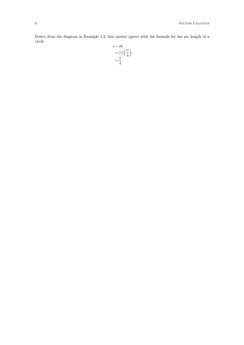
Notice from the diagram in Example 1.2, this answer agrees with the formula for the arc length of acircle
s = rθ
=(1)(
π
4
)
=π
4.
8 Vector Calculus

1.2 Review of partial differentiation
Recall for a function of one variable f(x), the derivative at x = a is given by
f ′(a) = limh→0
f (a+h)− f(a)
h(1.1)
and f ′(a) has the geometric interpretation as the slope of the tangent line to f(x) at x = a as maybe seen in the following diagram.
Example 1.9. If f(x) = x2 then f ′(x) = 2x. At the value x = 1, we have f ′(1) = 2 and so the slopeof the tangent to the point (1, 1) is equal to 2 as illustrated in the following diagram
The limit definition (1.1) is not usually used to compute derivatives, in practice derivatives arecomputed by a set of rules – power rule, product rule, quotient rule etc. Similarly, partial deriva-tives are defined using limits, but actually computed by using rules. The following are the defini-tions of partial derivatives of a function f(x, y) of two variables
Definition 1.10.
i. If f(x, y) is a function of two variables then the partial derivative of f with respect to
x at the point (a, b) is denoted as fx(a, b) or∂f
∂x(a, b) and is defined as
fx(a, b)= limh→0
f(a+h, b)− f(a, b)
h
ii. If f(x, y) is a function of two variables then the partial derivative of f with respect to
y at the point (a, b) is denoted as fy(a, b) or∂f
∂y(a, b) and is defined as
fy(a, b)= limh→0
f(a, b+h)− f(a, b)
h
Partial derivatives of a function of two variables are usually computed by the following
Rule for finding partial derivatives of f(x, y)
i. To find fx, treat y as a constant and differentiate with respect to x.
ii. To find fy, treat x as a constant and differentiate with respect to y.
Example 1.11. Let f(x, y) =x2y3. Find∂f
∂xand
∂f
∂y.
Answer: To find∂f
∂x, treat y as a constant in f(x, y) = x2y3 . One can imagine that y is equal to
some fixed constant, say y = 11. Therefore ′′f(x, y) = x2113′′ and now differentiate x2113 as usualwith respect to x to get (x2113)′=2x113.Now replace the 11 by y to get the answer
∂f
∂x= 2xy3.
1.2 Review of partial differentiation 9

Similarly to find∂f
∂y, treat x as a constant in f(x, y) = x2y3. As before, imagine that x is equal to a
fixed constant, say x = 7. Therefore f(x, y) = 72y3′′ and now differentiate 72y3 as usual with respectto y to get (72y3)′ =72 (3y2).Now replace the 7 by x to get the answer
∂f
∂y=x2(3y2) = 3x2y2.
Example 1.12. Let f(x, y) =x2cos(x + y). Find∂f
∂xand
∂f
∂y.
Answer: To find∂f
∂x, treat y as a constant in f(x, y) = x2cos(x + y), say y = 13. Then ′′f(x, y) =
x2cos(x + 13)′′ and this is a product of two functions, therefore we use the usual product rule to dif-ferentiate with respect to x
(x2cos(x+ 13))′=(x2)′cos(x+ 13) +x2(cos(x + 13)′)= 2x cos(x+ 13)−x2sin(x+ 13)
and replacing the 13 by y we have the answer
∂f
∂x= 2x cos(x + y)− x2sin(x + y).
To find∂f
∂y, treat x as a constant. In this case f(x, y) = x2cos(x + y) is a product of a constant x2
and a function cos(x+ y) and so it is not necessary to use product rule. We have the answer
∂f
∂y=x2 ∂
∂y(cos(x + y))
=x2(− sin(x+ y))
=− x2sin(x + y).
Recall that one obtains the second derivatived2f
dx2of a function f(x) of one variable by differenti-
ating the first derivative, for example
f(x) = sinx
⇒ df
dx= cosx
⇒ d2f
dx2=
d
dx
(
df
dx
)
=d
dx(cosx)
=− sinx.
Similarly, one obtains the second partial derivatives∂2f
∂x2,
∂2f
∂y2,
∂2f
∂x∂yand
∂2f
∂y∂xof a function f(x,
y) of two variables by taking the partial derivative of a first partial derivative∂f
∂xor
∂f
∂y. To be pre-
cise
∂2f
∂x2=
∂
∂x
(
∂f
∂x
)
∂2f
∂y2=
∂
∂y
(
∂f
∂y
)
∂2f
∂y∂x=
∂
∂y
(
∂f
∂x
)
∂2f
∂x∂y=
∂
∂x
(
∂f
∂y
)
.
10 Vector Calculus
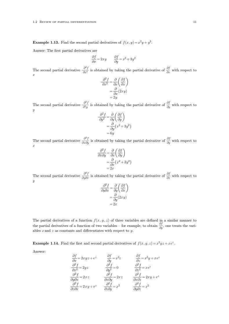
Example 1.13. Find the second partial derivatives of f(x, y)=x2y + y3.
Answer: The first partial derivatives are
∂f
∂x=2xy
∂f
∂y=x2 +3y2
The second partial derivative∂2f
∂x2is obtained by taking the partial derivative of
∂f
∂xwith respect to
x
∂2f
∂x2=
∂
∂x
(
∂f
∂x
)
=∂
∂x(2xy)
= 2y
The second partial derivative∂2f
∂2yis obtained by taking the partial derivative of
∂f
∂ywith respect to
y
∂2f
∂y2=
∂
∂y
(
∂f
∂y
)
=∂
∂y
(
x2 + 3y2)
= 6y
The second partial derivative∂2f
∂x∂yis obtained by taking the partial derivative of
∂f
∂ywith respect to
x
∂2f
∂x∂y=
∂
∂x
(
∂f
∂y
)
=∂
∂x
(
x2 +3y2)
= 2x
The second partial derivative∂2f
∂y∂xis obtained by taking the partial derivative of
∂f
∂xwith respect to
y
∂2f
∂y∂x=
∂
∂y
(
∂f
∂x
)
=∂
∂y(2xy)
= 2x
The partial derivatives of a function f(x, y, z) of three variables are defined in a similar manner to
the partial derivatives of a function of two variables – for example, to obtain∂f
∂y, one treats the vari-
ables x and z as constants and differentiates with respect to y.
Example 1.14. Find the first and second partial derivatives of f(x, y, z)= x2yz +xez.
Answer:∂f
∂x= 2xyz + ez ∂f
∂y=x2z
∂f
∂z=x2y +xez
∂2f
∂x2= 2yz
∂2f
∂y2= 0
∂2f
∂z2= xez
∂2f
∂y∂x=2xz
∂2f
∂x∂y=2xz
∂2f
∂x∂z=2xy + ez
∂2f
∂z∂x=2xy + ez ∂2f
∂z∂y=x2 ∂2f
∂y∂z= x2
1.2 Review of partial differentiation 11

We saw in Example 1.9 that the derivative f ′(a) can be interpreted as the slope of the tangent ofthe function f(x) at the point x = a. In a similar manner, if f(x, y) is a function of two variables
then the first partial derivatives∂f
∂x(a, b) and
∂f
∂y(a, b) may also be interpreted as slopes of lines
passing through the point corresponding to (x, y)= (a, b).
Recall that the graph of a function f(x, y) is obtained by plotting points (x, y, f (x, y)) in three–dimensional space. In this way, the graph of a function of two variables forms a surface in 3 dimen-sions. For example, the graph of the function f(x, y)= 1− x forms a surface that is a plane:
We illustrate the geometric interpretation of the partial derivatives∂f
∂x,
∂f
∂yby considering the
behaviour of the function f(x, y) = 1 − x at (x, y) = (1
2, 0). By taking partial derivatives, we have
that∂f
∂x
(
1
2, 0
)
=− 1∂f
∂y
(
1
2, 0
)
= 0.
Now notice that f(1
2, 0)=1− 1
2=
1
2. Therefore the point
(
1
2, 0, f(
1
2, 0)
)
=
(
1
2, 0,
1
2
)
lies on the graph of f(x, y) = 1− x as we see in the above diagram. The z − coordinate of(
1
2, 0,
1
2
)
is the function value f(1
2, 0) and corresponds to the height of the point
(
1
2, 0, f(
1
2, 0))
above the xy-
plane.
We now keep x =1
2fixed and change the y-value. Plotting such points f(
1
2, y) gives the line B on
the above diagram. Notice from the diagram that line B is parallel to the xy-plane, that is, thevalue of the function f does not change if we keep x =
1
2fixed and change the y-value. This corre-
sponds to∂f
∂y
(
1
2, 0
)
= 0
12 Vector Calculus

because the partial derivative∂f
∂y(1
2, 0) measures the rate at which at the function f is increasing as
the y-value changes while keeping x =1
2fixed.
Now keep y = 0 fixed and change the x-value. Plotting such points f(x, 0) gives the line A in theabove diagram. Notice that the height of the points on line A is decreasing as the x-values increase.This corresponds to
∂f
∂x
(
1
2, 0
)
=− 1
because the partial derivative measures the rate at which the function f is increasing as the x-valueincreases while keeping y =0 fixed.
1.2 Review of partial differentiation 13

1.3 Vector Fields
Definition 1.15.A vector field on the Cartesian plane R
2 is a function F that assigns a two dimensional vectorF (x, y) to each point (x, y). We may write F in terms of its component functions
F (x, y) =P (x, y)i+ Q(x, y)j.
Furthermore, the vector field F is said to be continuous if and only if each its component functionsis continuous.
Example 1.16. The following diagram is a plot of the vector field
F (x, y)=− yi+ xj
on the Cartesian plane. Notice that each point (x, y) on the Cartesian plane has a vector associatedto it.
Similarly, we may define vector fields in the three dimensional space R3.
Definition 1.17. A vector field on the three dimensional space R3 is a function F that assigns a
three dimensional vector F (x, y, z) to each point (x, y, z). We may write F in terms of its compo-nent functions
F (x, y, z)=P (x, y, z)i + Q(x, y, z)j + R(x, y, z)k.
Furthermore, the vector field F is said to be continuous if and only if each its component functionsis continuous.
1.3.1 Divergence and curl of a vector field
Definition 1.18. Let
F (x, y)= P (x, y)i+ Q(x, y)j
be a vector field on the Cartesian plane R2 where the first partial derivatives of the component func-
tions P and Q exist. Then the divergence of the vector field F is the function
div(F ) =∂P
∂x+
∂Q
∂y.
14 Vector Calculus

Example 1.19. Find the divergence of the following vector fields on the Cartesian plane R2
i. F (x, y)= 3i
ii. G(x, y)= 3x2i
Answer:
i.
div(F )=∂P
∂x+
∂Q
∂x
=∂
∂x(3)+
∂
∂x(0)
= 0ii.
div(G)=∂P
∂x+
∂Q
∂x
=∂
∂x(3x2)+
∂
∂x(0)
= 6x
The divergence of a vector field has the following interpretation. Consider a infinitesimally small boxof length ∆x and width ∆y located at the point (x, y)
Then the divergence of a vector field F at the point (x, y) can be viewed as the net flow of F out ofan infinitesimally small box located at the point (x, y).
Consider the two vector fields F and G of Example 1.19. Notice that the vector field F (x, y) = 3iis a constant vector field
so the net flow of F out of the small box located at the point (x, y) is zero, which agrees with theanswer div(F )= 0 obtained in Example 1.19.
1.3 Vector Fields 15

Notice however that the vector field G(x, y) = 3x2i is nonconstant, and that the length of the vectorsincreases as x increases. From the diagram below
we see that the vectors at one vertical side of the small box are longer than the vectors at the othervertical side. Hence one can regard the net flow out of the box as positive, which agrees with theanswer div(G)= 6x1.1 obtained in Example 1.19.
The following is the definition of the divergence of a three dimensional vector field.
Definition 1.20. Let
F (x, y, z)=P (x, y, z)i + Q(x, y, z)j + R(x, y, z)k
be a vector field on three dimensional space R3 where the first partial derivatives of the component
functions P , Q andR exist. Then the divergence of the vector field F is the function
div(F ) =∂P
∂x+
∂Q
∂y+
∂R
∂z.
The divergence of a three dimensional vector field can be expressed in an alternative form by the useof a differential operator
Definition 1.21. Let ∇ denote the vector differential operator
∇=∂
∂xi+
∂
∂yj +
∂
∂zk.
Then the divergence of the vector field
F (x, y, z)=P (x, y, z)i + Q(x, y, z)j + R(x, y, z)k
is given by the dot product of ∇ and F
div(F ) =∇.F
It is not hard to check that Definition 1.20 and Definition 1.21 are equivalent:
div(F )=∇.F
=
(
∂
∂xi+
∂
∂yj +
∂
∂zk
)
· (P (x, y, z)i + Q(x, y, z)j + R(x, y, z)k)
=∂
∂x(P )+
∂
∂y(Q)+
∂
∂z(R)
=∂P
∂x+
∂Q
∂y+
∂R
∂z.
1.1. For a box located at (x, y) where x > 0. If the box is located on the opposite side of the y − axis, then the vectorsreverse direction and our interpretation still holds.
16 Vector Calculus

Note that the divergence of three dimensional vector field has a similar interpretation to the diver-gence in two dimensions – div(F ) at the point (x, y, z) can be viewed as the net flow of F out of aninfinitesimally small cube located at the point (x, y, z).
Definition 1.22. Let
F (x, y, z)=P (x, y, z)i + Q(x, y, z)j + R(x, y, z)k
be a vector field on three dimensional space R3 where the first partial derivatives of the component
functions P , Q andR exist. Then the curl of the vector field F is the vector field on R3 defined by
curl (F )=∇×F
=
∣
∣
∣
∣
∣
∣
∣
i j k∂
∂x
∂
∂y
∂
∂z
P Q R
∣
∣
∣
∣
∣
∣
∣
=
(
∂R
∂y− ∂Q
∂z
)
i+
(
∂P
∂z− ∂R
∂x
)
j +
(
∂Q
∂x− ∂P
∂y
)
k.
Example 1.23. Find the curl of the vector field F (x, y, z)=xzi+xyzj − y2k.
Answer:
curl (F ) =∇×F
=
∣
∣
∣
∣
∣
∣
∣
∣
i j k∂
∂x
∂
∂y
∂
∂z
xz xyz − y2
∣
∣
∣
∣
∣
∣
∣
∣
=(− 2y −xy)i+ (x− 0)j + (yz − 0)k=(− 2y − xy)i +xj + yzk.
Note that at any specific point (x, y, z), curl (F ) is a three dimensional vector and so corresponds to
some specific direction in three dimensional space R3. Consider a small paddle that can rotate along
an axis. If the vector field F is viewed as the velocity of a liquid then curl (F ) at the point (x, y, z)would be the direction in which the axis of the paddle should be aligned in order to get the fastestcounterclockwise rotation at the point (x, y, z) .
1.3.2 Gradient of a function
Definition 1.24. If f(x, y) is a function of two variables defined on the Cartesian plane R2 where
the first partial derivatives of f(x, y) exist, then the gradient of the function, denoted as grad(f), isthe vector function defined as
grad(f)=∂f
∂xi+
∂f
∂yj.
Remark 1.25.
Note that grad(f) assigns a two dimensional vector
∂f
∂x(x0, y0)i+
∂f
∂y(x0, y0)j
to each point (x0, y0) of the Cartesian plane R2. It follows from Definition 1.15 that grad(f) is a
vector field and because of this, grad(f) is also referred to as the gradient vector field of f.
1.3 Vector Fields 17

Example 1.26. Let f(x, y) =x2 + y2. Then
grad(f)=∂
∂x(x2 + y2)i+
∂
∂y(x2 + y2)j
=2xi+ 2y j.
At any specific point (x, y), grad(f) is a vector that gives the direction of the maximum increase ofthe function f(x, y). Consider the following contour plot of the function f(x, y)=x2 + y2
Figure 1.1. Contour plot of f(x, y) =x2 + y2
Note that all points (x, y) on the circle labelled f = 1 have function value equal to 1. The point
(x, y) = (1/2, 3√
/2) is one such point on the circle f = 1. Notice that if we change the (x, y) valuesin the direction of arrow A, that is if we take (x, y) values along the circle f = 1, then the functionf(x, y) does not change value. In order to get the maximum increase in the function f(x, y) we mustmove in the direction perpendicular to the circle f =1; this is the direction specified by
grad(f)= 2xi+2y j
= i + 3√
jin the diagram.
Definition 1.27. Let (x, y) be a point on a curve C in the Cartesian plane R2 that has a well-
defined tangent vector T . Then any vector n at the point (x, y) that is perpendicular to the tangentvector T is called a normal vector to the curve C at the point (x, y).
Example 1.28. In Figure 1.1 above, the arrow A is a tangent vector to the curve f = 1 at the point(x, y)= (1/2, 3
√/2). The vector
grad(f)= i+ 3√
j
is an example of a normal vector to the curve f = 1 at the point (1/2, 3√
/2).
Definition 1.29. Let f(x, y) be a function of two variables and let c be a constant. The set ofpoints that satisfy
f(x, y)= c
called a level curve of the function f(x, y).
18 Vector Calculus

Example 1.30. Let f(x, y) =x2 + y2. Then the level curve
f(x, y)= 1
is the circle
x2 + y2 =1.
Notice that the three level curves f(x, y) = 1, f(x, y) = .49 and f(x, y) = .25 are shown in Figure 1.1above.
Theorem 1.31. Let f(x, y) = c be a level curve C in the Cartesian plane where f(x, y) is a differ-entiable function. Then if grad(f) at a point (x, y) is not the zero vector, then it is a normal vectorto the curve C at the point (x, y).
Example 1.32. Find a normal vector to the ellipse x2 + 4y2 =1 at the point(
1
2√ ,
1
2 2√)
.
Answer: Notice that the curve x2 +4y2 =1 is a level curve as it is in the form
f(x, y)= 1
where f(x, y)= x2 + 4y2. The gradient of the function f is
grad(f)=∂f
∂xi+
∂f
∂yj
=2xi+8yj
and at the point (x, y)=(
1
2√ ,
1
2 2√)
, grad(f) is equal to
grad(f)= 2xi+8yj
=2
2√ i+
8
2 2√ j
= 2√
i+2 2√
j
which, by Theorem 1.31 is a normal vector to x2 +4y2 =1 at the point(
1
2√ ,
1
2 2√)
.
Recall that the partial derivative∂f
∂x(x0, y0) measures the rate at which the function f is increasing
as the x-value increases while keeping the y − value fixed, in other words,∂f
∂x(x0, y0) gives the rate of
change in the function f as the (x, y) points move from (x0, y0) in the direction of the horizontalunit vector i; see Figure 1.2 below.
Similarly the partial derivative∂f
∂y(x0, y0) gives the rate of change in the function f as the (x, y)
points move from (x0, y0) in the direction of the vertical unit vector j as is also illustrated in Figure1.2 below.
1.3 Vector Fields 19

Figure 1.2. Diagram of the domain of the function f
If we wish to determine the rate at which a function changes as the (x, y) points move from a fixedpoint (x0, y0) in the direction of a unit vector that is not horizontal or vertical, then we shall needthe following definition.
Definition 1.33. The directional derivative of a function f(x, y) in the direction of a unitvector u at a point (x0, y0), denoted as Duf , is defined as the dot product
Duf = u · grad(f)
Example 1.34. Find the directional derivative of the function f(x, y) = x2 + y2 at the point (1, 2)in the direction i− j.
Answer: In the definition of the directional derivative, the direction is specified by a unit vector. Wefirst find the unit vector u parallel to i− j
u =i− j
length of i− j
=i− j
12 +(− 1)2√
=1
2√ i− 1
2√ j
The vector grad(f) at the point (x, y) = (1, 2) is
grad(f)=∂f
∂xi+
∂f
∂yj
=2xi+2yj
= 2i +4j
and the required directional derivative is
Duf = u · grad(f)
=
(
1
2√ i− 1
2√ j
)
· (2i+4j)
=− 2√
.
20 Vector Calculus

The gradient of a function f(x, y, z) of three variables is defined and has properties analogous to thegradient of a function of two variables.
Definition 1.35. If f(x, y, z) is a function of three variables, then the gradient of the function,denoted as grad(f), is the vector function defined as
grad(f) =∂f
∂xi+
∂f
∂yj +
∂f
∂zk.
Note that the vector differential operator of Definition 1.21 can be used to give an alternativeexpression of grad(f)
grad(f)=∇f .
Definition 1.36. Let f(x, y, z) be a function of three variabless and let c be a constant. The set ofpoints that satisfy
f(x, y, z)= c
called a level surface of the function f(x, y, z).
Example 1.37. Let f(x, y, z) =x2 + y2 + z2. Then the level surface S
f(x, y, z)= 1
is the sphere
x2 + y2 + z2 =1.
of radius 1 is illustrated in Figure 1.3 below.
Figure 1.3.
Definition 1.38. The tangent plane to a point P on a surface S is the plane that touches thesurface at the point P . A normal vector to a surface S at the point P is a vector that is perpen-dicular to the tangent plane at the point P .
Theorem 1.39. Let f(x, y, z) = a be a surface S in three dimensional space where f(x, y, z) is adifferentiable function. Then if grad(f) at a point (x, y, z) is not the zero vector, then it is a normalvector to the surface S at the point (x, y, z).
1.3 Vector Fields 21
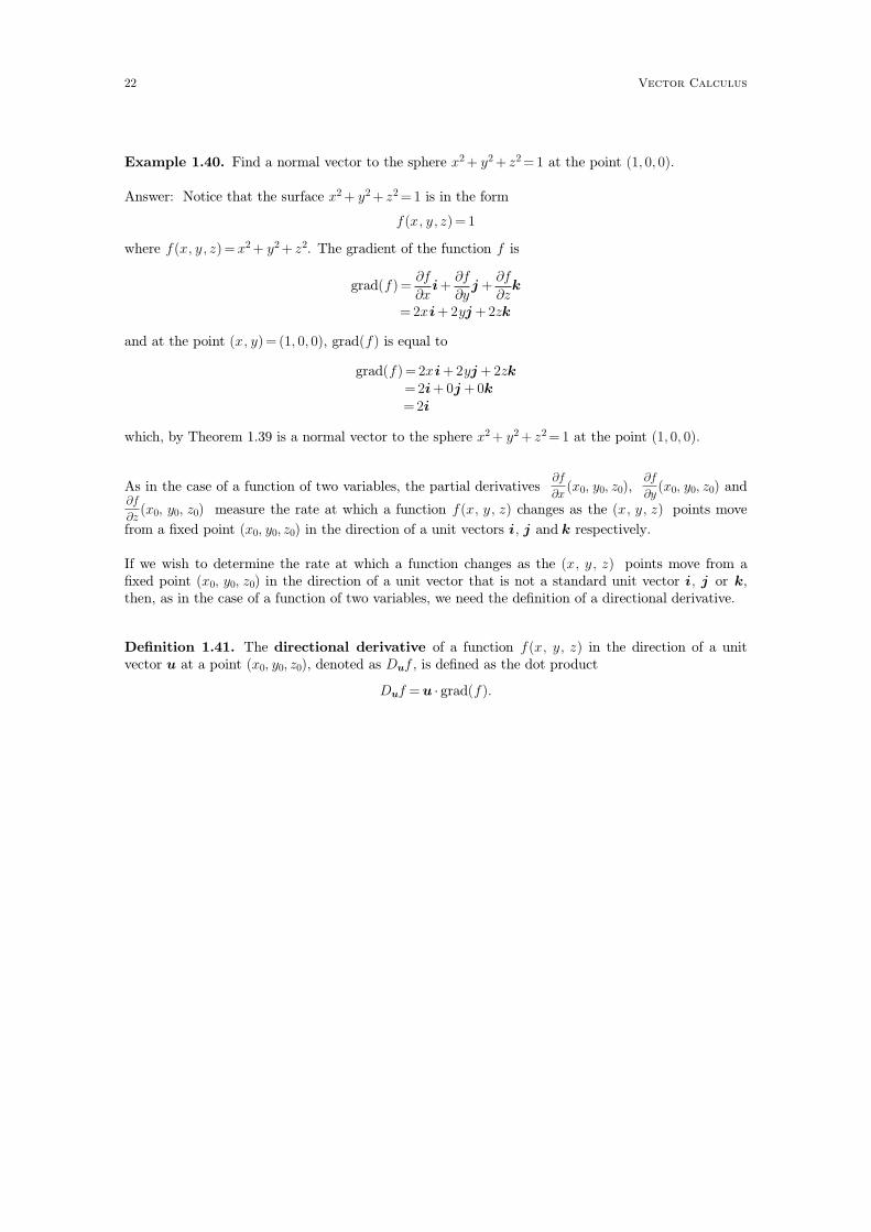
Example 1.40. Find a normal vector to the sphere x2 + y2 + z2 =1 at the point (1, 0, 0).
Answer: Notice that the surface x2 + y2 + z2 = 1 is in the form
f(x, y, z)= 1
where f(x, y, z)= x2 + y2 + z2. The gradient of the function f is
grad(f)=∂f
∂xi+
∂f
∂yj +
∂f
∂zk
=2xi+ 2yj +2zk
and at the point (x, y)= (1, 0, 0), grad(f) is equal to
grad(f)= 2xi +2yj + 2zk=2i+ 0j +0k=2i
which, by Theorem 1.39 is a normal vector to the sphere x2 + y2 + z2 = 1 at the point (1, 0, 0).
As in the case of a function of two variables, the partial derivatives∂f
∂x(x0, y0, z0),
∂f
∂y(x0, y0, z0) and
∂f
∂z(x0, y0, z0) measure the rate at which a function f(x, y, z) changes as the (x, y, z) points move
from a fixed point (x0, y0, z0) in the direction of a unit vectors i, j and k respectively.
If we wish to determine the rate at which a function changes as the (x, y, z) points move from afixed point (x0, y0, z0) in the direction of a unit vector that is not a standard unit vector i, j or k,then, as in the case of a function of two variables, we need the definition of a directional derivative.
Definition 1.41. The directional derivative of a function f(x, y, z) in the direction of a unitvector u at a point (x0, y0, z0), denoted as Duf , is defined as the dot product
Duf = u · grad(f).
22 Vector Calculus

1.4 Line integrals and double integrals
1.4.1 Line integrals
Definition 1.42. Let F (x, y) be a continuous vector field defined on the Cartesian plane and let C
be the smooth parametric curve
r(t)=x(t)i + y(t)j a6 t6 b.
Then the line integral of the vector field F along the curve C is
∫
C
F · dr =
∫
a
b
F (x(t), y(t)) · (x ′(t)i + y ′(t)j ) dt
A line integral∫
CF · dr can be interpreted as the work done on a particle by a force field F as it
travels on a path C. Consider the following example.
Example 1.43. Let F (x, y) = 3x2i be a vector field on the Cartesian plane. Calculate the followingline integrals
i.∫
C1F · dr where C1 is the curve
r(t) = (1 + t)i + j 06 t6 1
ii.∫
C2F · dr where C2 is the curve
r(t) = i+ (1 + t)j 06 t6 1.
Answer:
i.∫
C1
F · dr =
∫
a
b
F (x(t), y(t)) · (x′(t)i+ y ′(t)j ) dt
=
∫
0
1
F ((1 + t), 1) · ((1 + t) ′i+(1)′j ) dt
=
∫
0
1(
3(1 + t)2i)
· (1i+ 0j ) dt
=
∫
0
1
3(1 + t)2 dt
=[
(1 + t)3]
0
1
=8.ii.
∫
C2
F · dr =
∫
a
b
F (x(t), y(t)) · (x′(t)i+ y ′(t)j ) dt
=
∫
0
1
F (1, (1 + t)) · ((1)′i+ (1 + t)′j ) dt
=
∫
0
1(
3(1)2i)
· (0i+1j ) dt
=
∫
0
1
3i · (0i+1j ) dt
=
∫
0
1
0dt
=0.
1.4 Line integrals and double integrals 23

Figure 1.4 below is an illustration of the vector field F (x, y)= 3x2i and the two curves
C1: r(t) = (1 + t)i + j 06 t6 1
C2: r(t)= i +(1 + t)j 0 6 t6 1.
If we regard the vector field F as a force field then as C1 lies in the direction of F , we expect F toadd energy to a particle travelling along the path C1. This agrees with
∫
C1
F · dr = 8
in part i). However, the curve C2 is perpendicular to the direction of vector field and therefore F
does not add any energy to a particle travelling along C2 which agrees with the answer∫
C2
F · dr = 0.
in part ii).
Figure 1.4.
The definition of a line integral in three dimensional space is similar to the definition in the Carte-sian plane.
Definition 1.44. Let F (x, y, z) be a continuous vector field defined in three dimensional space andlet C be the smooth parametric curve
r(t)=x(t)i+ y(t)j + z(t)k a6 t6 b.
Then the line integral of the vector field F along the curve C is∫
C
F · dr =
∫
a
b
F (x(t), y(t), z(t)) · (x′(t)i + y ′(t)j + z ′(t)k ) dt.
Example 1.45. Evaluate∫
C
F · dr
where F is the vector field in three dimensional space
F (x, y, z)= xyi + yzj + zxk
and C is the parametric curve
r(t)= ti + t2j + t3k 06 t 6 1.
24 Vector Calculus

Answer: From Definition 1.44 above, we have
∫
C
F · dr =
∫
a
b
F (x(t), y(t), z(t)) · (x ′(t)i + y ′(t)j + z ′(t)) dt
=
∫
0
1
F (t, t2, t3) ·(
(t)′i+(t2)′j +(t3)′k)
dt
=
∫
0
1(
t3i+ t5j + t4k)
·(
1i +2tj + 3t2k)
dt
=
∫
0
1
(t3 +2t6 + 3t6)dt
=
[
t4
4+
5t7
7
]
0
1
=27
28.
1.4.2 Path independence and conservative vector fields
Definition 1.46. If C is a parametric curve in the Cartesian plane of the form
r(t) = f(t)i+ g(t)j where a6 t6 b,
then the initial point of C is given by the position vector r(a) and the terminal point of C isgiven by the position vector r(b). Similarly, one can define the initial and terminal points of a para-metric curve
r(t) = f(t)i+ g(t)j +h(t)k a 6 t6 b
in three dimensional space.
Example 1.47. Let F be the vector field
F (x, y)= y2 i +xj
and let C1 and C2 be the parametric curves defined as
C1: r(t)= (5t− 5)i+(5t− 3)j 06 t6 1
C2: r(t)= (4− t2)i + tj − 3 6 t6 2.
a) Sketch the curves C1 and C2 and verify that C1, C2 have the same initial and terminal point
b) By evaluating the respective line integrals, show that∫
C1
F · dr � ∫C2
F · dr .
Answer:
a) In the case of C1, we havex =5t− 5y = 5t− 3
.
Note that both x, y are linear functions of t and that the parameter t takes values in a finiteinterval 0 6 t 6 1. It follows that C1 is a line segment with initial point r(0) = ( − 5, − 3) andterminal point r(1)= (0, 2).
In the case of C2, the initial point is r( − 3) = ( − 5, − 3) and terminal point r(2) = (0, 2). Todetermine the shape of C2, we eliminate t from
x =4− t2
y = tto obtain
x =4− y2.
1.4 Line integrals and double integrals 25
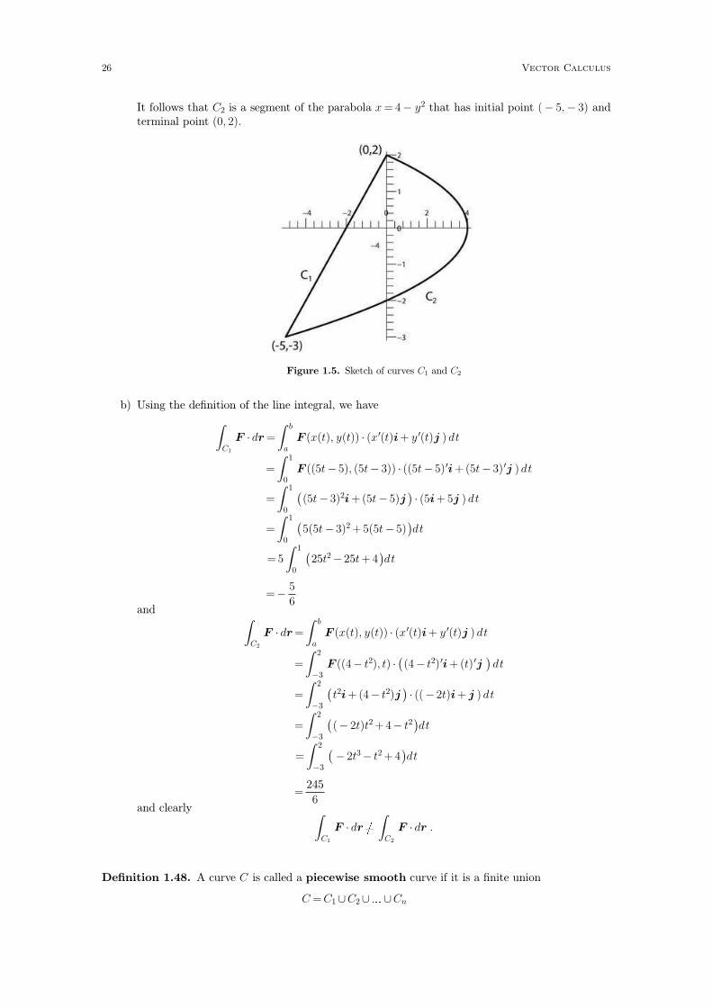
It follows that C2 is a segment of the parabola x = 4− y2 that has initial point (− 5,− 3) andterminal point (0, 2).
Figure 1.5. Sketch of curves C1 and C2
b) Using the definition of the line integral, we have
∫
C1
F · dr =
∫
a
b
F (x(t), y(t)) · (x′(t)i+ y ′(t)j ) dt
=
∫
0
1
F ((5t− 5), (5t− 3)) · ((5t− 5)′i +(5t− 3)′j ) dt
=
∫
0
1(
(5t− 3)2i +(5t− 5)j)
· (5i+ 5j ) dt
=
∫
0
1(
5(5t− 3)2 +5(5t− 5))
dt
=5
∫
0
1(
25t2− 25t+ 4)
dt
=− 5
6and
∫
C2
F · dr =
∫
a
b
F (x(t), y(t)) · (x′(t)i+ y ′(t)j ) dt
=
∫
−3
2
F ((4− t2), t) ·(
(4− t2)′i +(t)′j)
dt
=
∫
−3
2(
t2i+ (4− t2)j)
· ((− 2t)i+ j ) dt
=
∫
−3
2(
(− 2t)t2 +4− t2)
dt
=
∫
−3
2(
− 2t3− t2 +4)
dt
=245
6and clearly
∫
C1
F · dr � ∫C2
F · dr .
Definition 1.48. A curve C is called a piecewise smooth curve if it is a finite union
C =C1∪C2∪� ∪Cn
26 Vector Calculus

of smooth curves C1, C2,� , Cn such that the terminal point of Ci is the initial point of Ci+1.
Figure 1.6. A piecewise smooth C = C1∪C2∪C3
A line integral along a piecewise smooth curve is obtained by adding the line integrals of its indi-vidual pieces.
Definition 1.49. Let C = C1 ∪ C2 ∪ � ∪Cn be a piecewise smooth curve. Then the line integral ofthe vector field F along the curve C is
∫
C
F · dr =
∫
C1
F · dr +
∫
C2
F · dr +� +
∫
Cn
F · dr
Definition 1.50. A line integral∫
C
F · dr
is said to be independent of path if∫
C
F · dr =
∫
C ′
F · dr
for any piecewise smooth curve C ′ which has the same initial point and terminal point as the curveC.
Example 1.51. Consider curves C1, C2 and the line integral∫
C1
F · dr
as defined in Example 1.47. This line integral is not independent of path as C2 has the same initialand terminal points as C1 but
∫
C1
F · dr � ∫C2
F · dr .
Recall from Remark 1.25 that the gradient grad(f) of a function f(x, y) is in fact a vector field.
Definition 1.52. Let F be a vector field defined on Rn1.2. Then F is said to be a conservative
vector field if there exists a function f such that
F = grad(f).
For such a case, f is called a potential function for the vector field F. 1.3
1.2. In this class we consider only the cases of n =2 (the Cartesian plane) and n =3 (three dimensional space)
1.3. A different definition F = − grad(f) is used in physics; with this alternative definition, the function f gives a moreaccurate physical interpretation of the work done by an outside force in moving against the vector field. In this class, we usethe definition F = grad(f ).
1.4 Line integrals and double integrals 27

The above is the standard definition of a conservative vector field; however it is not a practicalmethod of determining whether or not a vector field is conservative. A more useful criterion forvector fields in R
2 is the following
Theorem 1.53. Let
F (x, y) =P (x, y)i+ Q(x, y)j.
be a vector field defined on R2 where the component functions P and Q have continuous first partial
derivatives. Then F is conservative if and only if
∂P
∂y=
∂Q
∂x.
Example 1.54. Show that the vector field
F (x, y)= (6x +5y)i+ (5x +4y)j
is conservative and determine a potential function for F (x, y).
Answer: In this case
P (x, y) = 6x +5y
Q(x, y)= 5x+ 4yand
∂P
∂y=5 =
∂Q
∂x
so it follows that F is conservative. Let f be a potential function for F . Then
grad(f)= F
⇒ ∂f
∂xi+
∂f
∂yj =(6x+ 5y)i +(5x+ 4y)j
⇒
∂f
∂x=6x+ 5y
∂f
∂y=5x +4y
. (1.2)
Using partial integration1.4 to integrate the first equation of (1.2) with respect to x, we have
f(x, y)= 3x2 +5xy + C(y). (1.3)
The function C(y) can be determined by differentiating equation (1.3) with respect to y and usingthe second equation of (1.2)
∂f
∂y=5x +C ′(y)= 5x+ 4y
⇒C ′(y)= 4y
⇒C(y)= 2y2 + K
where K is a constant of integration. We therefore have
f(x, y)= 3x2 +5xy +2y2 + K
and by choosing K = 0 we have that f = 3x2 + 5xy + 2y2 is a potential function for the vector fieldF .
The following result specifies exactly what conditions are required for a line integral in Rn to be
independent of path.
1.4. see Example 1.59 on page 31
28 Vector Calculus

Theorem 1.55. Let F be a vector field on Rn. Then the line integral∫
C
F · dr
is independent of path if and only if F is a conservative vector field.
Furthermore, the value of a line integral that is independent of path can be determined from theendpoints of the curve and a potential function of the vector field
Theorem 1.56. (Fundamental Theorem of Line Integrals) Let F be a vector field defined onR
n and∫
CF · dr be a line integral that is independent of path. Then
∫
C
F · dr = f(r2)− f(r1)
where f is a potential function for the the vector field F and r1, r2 are respectively the initial andterminal points of the curve C.
Example 1.57. Let F be the vector field
F (x, y, z) =x3y4 i+x4y3j
and let C be the parametric curve defined as
C: r(t)= t√
i+ (1 + t3)j 06 t6 1.
a) Show that F is a conservative vector field
b) Find a potential function for F
c) Use the potential function of part (b) to evaluate the line integral∫
CF · dr.
Answer:
a) The given vector field is of the form F = P (x, y)i+ Q(x, y)j where
P (x, y) =x3y4
Q(x, y)= x4y3 .
As∂P
∂y=4x3y3 =
∂Q
∂xso it follows that F is conservative.
b) Let f be a potential function for F . Then
grad(f) =F
⇒ ∂f
∂xi+
∂f
∂yj =x3y4 i+x4y3j
⇒
∂f
∂x=x3y4
∂f
∂y=x4y3
. (1.4)
By partially integrating the first equation of (1.4) with respect to x, we have
f(x, y) =x4y4
4+ C(y). (1.5)
The function C(y) can be determined by differentiating equation (1.5) with respect to y andusing the second equation of (1.2)
∂f
∂y= x4y3 +C ′(y) =x4y3
⇒C ′(y)= 0
⇒C(y)=K
1.4 Line integrals and double integrals 29

where K is a constant of integration. We have
f(x, y)=x4y4
4+K
and by choosing K =0 we have that f =x4y4
4is a potential function for the vector field F .
c) Using the parametric definition of C, we have that the initial and terminal points of C are
r1 = r(0)= (0, 1)
r2 = r(1)= (1, 2)
and from Theorem 1.56∫
C
F · dr = f(r2)− f(r1)
= f(1, 2)− f(0, 1)
=1424
4− 0414
4=4.
1.4.3 Double integrals
We give the definition of a double integral over a rectangular region R and then state a theorem thatgives a procedure for evaluating double integrals over a rectangular region. We then note that adouble integral may be interpreted as a volume. Finally we explain the evaluation of double inte-grals over Type I , Type II and circular regions.
Definition 1.58. Let R be a rectangular region in the Cartesian plane defined by
R = {(x, y)| a6 x6 b, c6 y 6 d}.Divide the rectangular region R into subrectangles by partitioning the intervals a 6 x 6 b and c 6 y 6
d :
a =x0 <x1 <� <xm = b
c = y0 < y1 <� < yn = d
and define the subrectangle Rij as
Rij = {(x, y)|xi−1 6x 6xi , yj−1 6 y 6 yj}
30 Vector Calculus
Choose points (xij∗ , yij
∗ ) in each subrectangle Rij. Let ∆Aij denote the area of the subrectangle Rij
and let∥
∥P∥
∥ denote the length of the largest diagonal of all subrectangles (note that as we take
smaller subrectangles of R we have that∥
∥P∥
∥→ 0). Then the double integral of the function f(x,
y) over the rectangular region R is defined to be the limit∫ ∫
R
f(x, y)dA = lim‖P ‖→0
∑
i=1
m∑
j=1
n
f(xij∗ , yij
∗ )∆Aij
if this limit exists.
The above definition is not usually used to evaluate double integrals. We shall give a method of eval-uating double integrals based on the following procedure of partial integration.
Example 1.59. (of partial integration)
∫
1
2
xy dy =
[
xy2
2
]
y=1
y=2
=x22
2− x12
2
=3x
2.
Notice in the above procedure of partial integration we
• integrate a function of two variables with respect to y
• treat x as a constant when integrating
• the answer∫
1
2
xy dy =3x
2is a function of x.
We can also integrate partially with respect to x:
Example 1.60.∫
3
4
cos(xy) dy =
[
sin(xy)
y
]
x=3
x=4
=sin(4y)
y− sin(3y)
y
and notice in this case our answer is a function of y.
Using the procedure of partial integration and the following theorem we can evaluate double inte-grals over rectangular regions.
Theorem 1.61. (Fubini’s Theorem) If the function f(x, y) is continuous at each point in a rect-angular region
R = {(x, y)| a6 x6 b, c6 y 6 d}then
∫ ∫
R
f(x, y)dA =
∫
a
b(
∫
c
d
f(x, y)dy
)
dx =
∫
c
d(
∫
a
b
f(x, y)dx
)
dy. (1.6)
Note that the integrals within the brackets of (1.6) are evaluated by partial integration. Also noticethat (1.6) implies that the double integral over a rectangular region can be obtained by integratingwith respect to y and then x or integrating with respect to x and then y.
Example 1.62. Evaluate the double integral∫ ∫
R
x2y dA
1.4 Line integrals and double integrals 31

where R is the rectangular region
R = {(x, y)| 0 6x 6 3, 16 y 6 2}.
Answer: By Fubini’s Theorem∫ ∫
R
x2y dA =
∫
0
3( ∫
1
2
x2ydy
)
dx
=
∫
0
3[
x2 y2
2
]
y=1
y=2
dx
=
∫
0
3(
x2 22
2− x2 12
2
)
dx
=
∫
0
3 3x2
2dx
=
[
x3
2
]
x=0
x=3
=27
2.
Notation 1.63.
i. The integral∫
a
b(
∫
c
d
f(x, y)dy
)
dx
is usually denoted as∫
a
b ∫
c
d
f(x, y)dydx.
ii. Similarly, the integral∫
c
d(
∫
a
b
f(x, y)dx
)
dy
is usually denoted as∫
c
d ∫
a
b
f(x, y)dxdy.
Recall that the graph of a function f(x, y) forms a surface in three dimensional space. Given a func-tion f(x, y)> 0 for each point (x, y) in a rectangular domain R, then the double integral
∫ ∫
R
f(x, y)dA
can be interpreted as the volume between the graph of f(x, y) and the rectangle R lying in the xy −plane
32 Vector Calculus

We now consider double integrals over regions in the Cartesian plane that are not rectangular.
Definition 1.64.
i. A Type I region is a region in the Cartesian plane that may be described as
R = {(x, y)| a6 x6 b, f(x)6 y 6 g(x)}
where f(x) and g(x) are continuous functions of x.
ii. A Type II region is a region in the Cartesian plane that may be described as
R = {(x, y)| k(y) 6x 6 h(y), c 6 y 6 d}
where k(y) and h(y) are continuous functions of y.
Figure 1.7.
As in the evaluation of a double integral over a rectangular region, evaluating double integrals overType I and Type II regions requires the use of partial integration. Note that for a Type I region,the integration is done with respect to the y variable first and then with respect to x variable. For aType II region, the integration is done with respect to the y variable first and then with respect to x
variable.
Theorem 1.65.
i. If the function f(x, y) is continuous at each point in a Type I region
R = {(x, y)| a6 x6 b, g(x)6 y 6 f(x)}then
∫ ∫
R
f(x, y)dA =
∫
a
b(
∫
g(x)
f(x)
f(x, y)dy
)
dx
ii. If the function f(x, y) is continuous at each point in a Type II region
R = {(x, y)| k(y) 6x 6 h(y), c 6 y 6 d}then
∫ ∫
R
f(x, y)dA =
∫
c
d(
∫
k(y)
h(y)
f(x, y)dx
)
dy.
1.4 Line integrals and double integrals 33

Example 1.66. Evaluate the double integral
∫ ∫
R
x dA
where R = {(x, y)| 06 x6 1, 06 y 6 1− x2√
}.
Answer: Notice that R is a Type I region. Then
∫ ∫
R
xdA =
∫
0
1(
∫
0
1−x2√
xdy
)
dx
=
∫
0
1
[xy]y=0y= 1−x2
√dx
=
∫
0
1 (
x 1− x2√
−x(0))
dx
=
∫
0
1
x 1− x2√
dx
=
[
− (1−x2)3
2
3
]
x=0
x=1
=1
3.
Example 1.67. Evaluate the double integral
∫ ∫
R
xy dA
where R is the region bounded by the line x= y +1 and the parabola x =y2
2− 3.
Answer: By solving the equations
x= y +1
x=y2
2− 3
⇒ y +1 =y2
2− 3 ⇒ y =− 2, 4
and we see that the line x = y + 1 and the parabola x =y2
2− 3 intersect at the points ( − 1,− 2) and
(5, 4):
34 Vector Calculus

From the above diagram we can write R as
R = {(x, y)|y2
2− 3 6 x 6 y + 1, − 2 6 y 6 4}
and so the region R is of Type II . Then
∫ ∫
R
xy dA =
∫
−2
4
∫
y2
2−3
y+1
xy dx
dy
=
∫
−2
4[
x2y
2
]
x=y2
2−3
x=y+1
dy
=1
2
∫
−2
4(
(y +1)2y −(
y2
2− 3
)2
y
)
dy
=1
2
∫
−2
4(
y3 +2y2 + y − y5
4+3y3− 9y
)
dy
=1
2
∫
−2
4(
− y5
4+4y3 +2y2− 8y
)
dy
= 36.
Some regions in the Cartesian plane are more easily described by the use of polar coordinates.
Definition 1.68. A polar rectangle is a region in the Cartesian plane that may be described inpolar coordinates (r, θ) as
R = {(r, θ)| θ1 6 θ 6 θ2, a 6 r 6 b}
where a and b are real constants such that 06 a < b.
Figure 1.8.
Example 1.69. Express the following region
R = {(x, y)| 96 x2 + y2 6 25, x> 0, y > 0}as a polar rectangle.
Answer: The equations
x2 + y2 =9
x2 + y2 = 25
describe circles of radius 3 and 5 respectively that have the origin as center. Therefore the inequali-ties
96 x2 + y2 6 25, x > 0 and y > 0
1.4 Line integrals and double integrals 35

describe points that lie between the circles and in the first quadrant
and so we can write R as a polar rectangle
R = {(r, θ)| 06 θ 6π
2, 36 r 6 5}.
We shall use the following theorem to evaluate double integrals over regions in the Cartesian planethat are polar rectangles. Notice that the following theorem is a conversion of a double integral inxy − coordinates to a double integral in polar coordinates.
Theorem 1.70. If the function f(x, y) is continuous at each point in a polar rectangle
R = {(r, θ)| θ1 6 θ 6 θ2, a 6 r 6 b}then
∫ ∫
R
f(x, y)dA =
∫
θ1
θ2
(
∫
a
b
f(r cosθ, r sinθ)rdr
)
dθ.
Example 1.71. Evaluate the following double integral
∫ ∫
R
(
1− (x2 + y2))
dA
where R = {(x, y)| 06x2 + y2 6 1} by converting to polar coordinates.
Answer: The region R is the unit disc
and so we can write R as a polar rectangle
R = {(r, θ)| 06 θ 6 2π, 06 r 6 1}.
36 Vector Calculus

From Theorem 1.70, we have
∫ ∫
R
(
1− (x2 + y2))
dA =
∫
0
2π( ∫
0
1
(1− (r2cos2θ + r2sin2θ))rdr
)
dθ
=
∫
0
2π( ∫
0
1
(1− r2)rdr
)
dθ
=
∫
0
2π( ∫
0
1
(r − r3 )dr
)
dθ
=
∫
0
2π[
r2
2− r4
4
]
0
1
dθ
=
∫
0
2π 1
4dθ
=π
2.
1.5 Green’s theorem
Definition 1.72.
i. A parametric curve C is called closed if its terminal point coincides with its initial point.
ii. A simple curve C is a curve that does not intersect itself anywhere between its endpoints.
Figure 1.9. Examples of curves
Convention: A positive orientation of a simple closed curve C refers to a counterclockwise traversalof C.
Theorem 1.73. (Green’s Theorem) Let C be a positively oriented, piecewise smooth, simpleclosed curve in the Cartesian plane. Let D be the region bounded by C. Let F be the vector field
F (x, y)= P (x, y)i+ Q(x, y)j
where P (x, y) and Q(x, y) have continuous partial derivatives on an open region that contains D.Then
∫
C
F · dr =
∫ ∫
D
(
∂Q
∂x− ∂P
∂y
)
dA
1.5 Green’s theorem 37
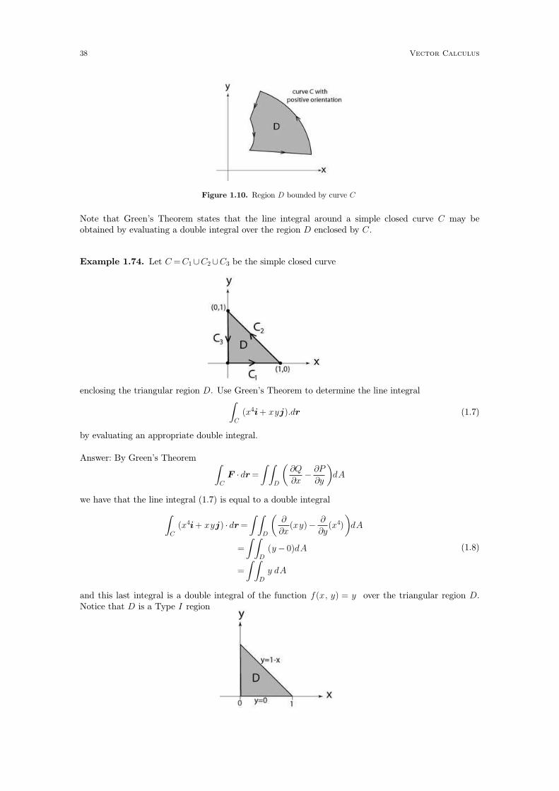
Figure 1.10. Region D bounded by curve C
Note that Green’s Theorem states that the line integral around a simple closed curve C may beobtained by evaluating a double integral over the region D enclosed by C.
Example 1.74. Let C =C1∪C2∪C3 be the simple closed curve
enclosing the triangular region D. Use Green’s Theorem to determine the line integral∫
C
(x4i+ xyj).dr (1.7)
by evaluating an appropriate double integral.
Answer: By Green’s Theorem∫
C
F · dr =
∫ ∫
D
(
∂Q
∂x− ∂P
∂y
)
dA
we have that the line integral (1.7) is equal to a double integral
∫
C
(x4i+ xyj) · dr =
∫ ∫
D
(
∂
∂x(xy)− ∂
∂y(x4)
)
dA
=
∫ ∫
D
(y − 0)dA
=
∫ ∫
D
y dA
(1.8)
and this last integral is a double integral of the function f(x, y) = y over the triangular region D.Notice that D is a Type I region
38 Vector Calculus

that is, we can describe the region D as the set
D = {(x, y)| 06 x6 1, 06 y 6 1− x}and therefore
∫ ∫
D
y dA =
∫
0
1 ∫
0
1−x
y dy dx (1.9)
Substituting (1.9) into (1.8) we have∫
C
(x4i + xyj) · dr =
∫ ∫
D
y dA
=
∫
0
1 ∫
0
1−x
y dy dx
and notice that this is the point of Green’s theorem – for a simple closed curve C, a line integralaround C is equal to a double integral over the region enclosed by C
∫
C
(x4i+ xyj).dr =
∫
0
1 ∫
0
1−x
y dy dx
and we can evaluate this double integral by using partial integration
∫
C
(x4i+ xyj).dr =
∫
0
1 ∫
0
1−x
y dy dx
=
∫
0
1[
y2
2
]
y=0
y=1−x
dx
=
∫
0
1 (1− x)2
2dx
=
[
− (1− x)3
6
]
0
1
=1
6
1.6 Surface integrals
1.6.1 Parametric surfaces
Recall that some curves C in three dimensional space can be described parametrically
C: r(t)= x(t)i+ y(t)j + z(t)k a6 t6 b,
for example the curve shown below
1.6 Surface integrals 39

may be written parametrically as
r(t)= ti+ tj + (1− t)k 06 t6 1.
We now describe surfaces in three dimensional space by the use of vector functions r(u, v) of twoparameters u and v.
Definition 1.75. A parametric surface S in three dimensional space is obtained by specifying x,y and z to be continuous functions of parameters u and v
x= f(u, v)y = g(u, v)z =h(u, v)
where (u, v) ∈ R and R is a region in the uv − plane. The parametric surface S can be written invector form
r(u, v)= f(u, v)i+ g(u, v)j +h(u, v)k (u, v)∈R.
Example 1.76. Let S be the (truncated) plane defined by y =1, 06x, z 6 1.
Then we can describe S a parametric surface by
r(u, v)=ui+ j + vk (u, v)∈R.
where R is the region {(u, v)|06 u, v 6 1}
in the uv −plane. Notice that each point (u, v) of R defines a unique point in S.
Example 1.77. Describe the cylinder S
x2 + y2 =4, 06 z 6 3.
as a parametric surface.
40 Vector Calculus
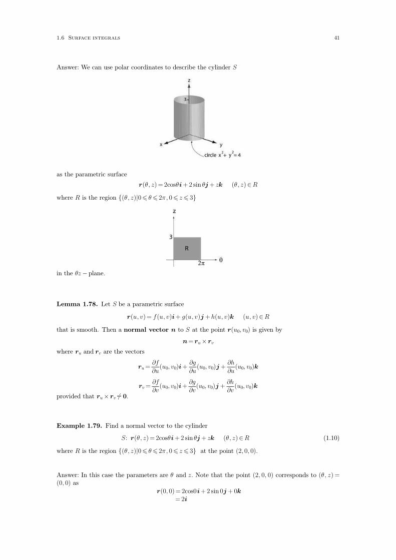
Answer: We can use polar coordinates to describe the cylinder S
as the parametric surface
r(θ, z) = 2cosθi +2 sin θj + zk (θ, z)∈R
where R is the region {(θ, z)|06 θ 6 2π, 06 z 6 3}
in the θz − plane.
Lemma 1.78. Let S be a parametric surface
r(u, v)= f(u, v)i+ g(u, v)j +h(u, v)k (u, v)∈R
that is smooth. Then a normal vector n to S at the point r(u0, v0) is given by
n= ru× rv
where ru and rv are the vectors
ru =∂f
∂u(u0, v0)i+
∂g
∂u(u0, v0)j +
∂h
∂u(u0, v0)k
rv =∂f
∂v(u0, v0)i+
∂g
∂v(u0, v0)j +
∂h
∂v(u0, v0)k
provided that ru× rv� 0.
Example 1.79. Find a normal vector to the cylinder
S: r(θ, z) = 2cosθi +2 sin θj + zk (θ, z)∈R (1.10)
where R is the region {(θ, z)|06 θ 6 2π, 06 z 6 3} at the point (2, 0, 0).
Answer: In this case the parameters are θ and z. Note that the point (2, 0, 0) corresponds to (θ, z) =(0, 0) as
r(0, 0)= 2cos0i+2 sin 0j + 0k= 2i
1.6 Surface integrals 41

The vector functions rθ(θ, z) and rz(θ, z) are obtained by differentiating (1.10) partially with respectto θ and z respectively
rθ(θ, z)=− 2sinθi+2 cos θj +0k
rz(θ, z) = 0i+0j +1k
and at (θ, z)= (0, 0)rθ(0, 0)= 2j
rz(0, 0)=k
and the normal vector at the point (2, 0, 0) is
n= rθ(0, 0)× rz(0, 0)=2j ×k
= 2i
1.6.2 Surface integrals
Definition 1.80. Let S be a smooth parametric surface
r(u, v)=x(u, v)i+ y(u, v)j + z(u, v)k (u, v)∈R
where R is a region in the uv − plane and let f(x, y, z) be a continuous function defined on S. Thenthe surface integral of the function f(x, y, z) over the surface S is
∫ ∫
S
f(x, y, z) dS =
∫ ∫
R
f(x(u, v), y(u, v), z(u, v)) |ru× rv | dA (1.11)
Note that equation (1.11) defines a surface integral to be equal to a double integral over a region R
in the uv − plane where u and v are the parameters of the surface S.
Example 1.81. Evaluate the surface integral∫ ∫
S
(x2y + z2) dS
where S is the part of the cylinder x2 + y2 =9 that lies between the plane z = 0 and z =2.
42 Vector Calculus

Answer: Our definition (1.11) of a surface integral requires that the surface S
be given in parametric form:
S: r(θ, z) = 3cosθi+3 sin θj + zk (θ, z)∈R (1.12)
where R is the region {(θ, z)|0 6 θ 6 2π, 0 6 z 6 2}. Note in this case we use the parameters r and θ
instead of u and v. The x, y and z components of S are
x=3cosθ y =3 sin θ z = z.
The vectors rθ and rz are
rθ =∂x
∂θi+
∂y
∂θj +
∂z
∂θk =− 3sinθi +3cosθj +0k
rz =∂x
∂zi+
∂y
∂zj +
∂z
∂zk = 0i +0j +k
and we have
rθ ×rz = (− 3sinθi+ 3cosθj)×k
=
∣
∣
∣
∣
∣
∣
i j k
− 3sinθ 3cos θ 00 0 1
∣
∣
∣
∣
∣
∣
=3cos θ i +3 sinθj
and therefore
|rθ × rz |= |3cos θ i+3 sinθj |
= 9cos2 θ +9 sin2θ√
= 3.
From the definition of a surface integral
∫ ∫
S
(x2y + z2) dS =
∫ ∫
R
f(x(θ, z), y(θ, z), z(θ, z)) |rθ × rz | dA
=
∫ ∫
R
(
(3cosθ)2(3sinθ)+ z2)
3 dA
= 3
∫ ∫
R
(
27cos2θ sinθ + z2)
dA
This last integral is a double integral of the function f(θ, z) = 27cos2θ sinθ + z2 over the rectangular
region R
1.6 Surface integrals 43

in the θz − plane. Therefore
∫ ∫
S
(x2y + z2) dS =3
∫ ∫
R
(
27cos2θ sinθ + z2)
dA
= 3
∫
0
2π ∫
0
2(
27cos2θ sinθ + z2)
dzdθ
= 3
∫
0
2π[
27cos2θ sinθz +z3
3
]
0
2
dθ
=3
∫
0
2π(
54cos2θ sinθ +8
3
)
dθ
=3
[
− 54cos3θ
3+
8θ
3
]
0
2π
(use substitution u = cos θ)
= 16π
A surface integral of a function f over a surface S can be interpreted as follows. Suppose that a sur-face S is subdivided into n smaller surfaces Si.
Choose a point (xi∗, yi
∗, zi∗) on each smaller surface Si. Let ∆Ai be the area of the small surface Si
and multiply this area by the value f(xi∗, yi
∗, zi∗) of the function f at the point (xi
∗, yi∗, zi
∗). Hence wehave a ‘weighted’ area
f(xi∗, yi
∗, zi∗)∆Ai
for each of the n smaller surfaces Si of the entire surface S. Then the surface integral of the functionf over the surface S is approximately the sum of each of the weighted areas for the Si
∫ ∫
S
f(x, y, z) dS ≃∑
i=1
n
f(xi∗, yi
∗, zi∗)∆Ai (1.13)
and if the number n of smaller surfaces Si gets larger then the approximation (1.13) gets better, sowe have
∫ ∫
S
f(x, y, z) dS = limn→∞
∑
i=1
n
f(xi∗, yi
∗, zi∗)∆Ai . (1.14)
Notice that if the function f(x, y, z) = 1 then from (1.14) we have
∫ ∫
S
1 dS = limn→∞
∑
i=1
n
∆Ai
and the right side of (1.14) is nothing but the sum of the areas of each of the smaller surfaces Si.This sum is obviously equal to the surface area of S. Therefore we have the following lemma
44 Vector Calculus

Lemma 1.82. The surface integral of the constant function f = 1 over the surface S is equal to thesurface area of S
∫ ∫
S
1 dS = surface area of S.
Example 1.83. Find the surface area of the truncated plane S
r(u, v)=ui+ j + vk (u, v)∈R.
where R is the region {(u, v)|06 u, v 6 1}.
Answer: The surface S is shown in the following diagram
(see Example 1.76). Clearly the surface area of S is equal to 1; let us verify this by evaluating thesurface integral
∫ ∫
S
1 dS.
The x, y and z components of S are
x= u y =1 z = v.
The vectors ru and rv are
ru =∂x
∂ui +
∂y
∂uj +
∂z
∂uk = i+0j +0k
rv =∂x
∂vi+
∂y
∂vj +
∂z
∂vk = 0i+0j +k
and we have
ru×rv = i×k
=
∣
∣
∣
∣
∣
∣
i j k
1 0 00 0 1
∣
∣
∣
∣
∣
∣
=− j
and so
|ru× rv |= |− j |=1
From the definition of a surface integral
∫ ∫
S
1 ds =
∫ ∫
R
1 |ru ×rv | dA
=
∫ ∫
R
1 dA
1.6 Surface integrals 45

This last integral is a double integral of the function f(u, v)= 1 over the rectangular region R
in the uv − plane. Therefore
∫ ∫
S
1 dS =
∫ ∫
R
1 dA
=
∫
0
1 ∫
0
1
1dudv
=
∫
0
1
[u]01dv
=
∫
0
1
(1− 0)dv
=
∫
0
1
1dv
=1
which agrees with our expected answer.
Recall that the graph of a function g(x, y) forms a a surface in three dimensional space. Let R be aregion in the xy − plane and let S be the surface formed as the image of the region R in the graph ofg(x, y):
Then the following lemma expresses a surface integral of a function f(x, y, z) over such a surface S
in terms of the function g(x, y).
Lemma 1.84. Let R be a region in the xy − plane and let S be the image of R in the graph of afunction g(x, y). Then the surface integral of the function f(x, y, z) over the surface S is equal to adouble integral over the region R in the xy − plane:
∫ ∫
S
f(x, y, z) dS =
∫ ∫
R
f(x, y, g(x, y)) 1 +
(
∂g
∂x
)2
+
(
∂g
∂y
)2√
dA
Proof. The surface S can be written parametrically as
r(x, y)= xi+ yj + g(x, y)k (x, y)∈R
46 Vector Calculus

with parameters x and y. The vectors rx and ry are
rx =∂
∂x(x)i+
∂
∂x(y)j +
∂
∂x(g(x, y))k = i+0j +
∂g
∂xk
ry =∂
∂y(x)i +
∂
∂y(y)j +
∂
∂y(g(x, y))k =0i+ j +
∂g
∂yk
and therefore
rx ×ry =
(
i+∂g
∂xk
)
×(
j +∂g
∂yk
)
=
∣
∣
∣
∣
∣
∣
∣
∣
∣
i j k
1 0∂g
∂x
0 1∂g
∂y
∣
∣
∣
∣
∣
∣
∣
∣
∣
=− ∂g
∂xi− ∂g
∂yj + k
hence
|rx ×ry |=∣
∣
∣
∣
− ∂g
∂xi− ∂g
∂yj +k
∣
∣
∣
∣
= 1 +
(
∂g
∂x
)2
+
(
∂g
∂y
)2√
and from the parametric definition of a surface integral in Definition 1.80 we have∫ ∫
S
f(x, y, z) dS =
∫ ∫
R
f(x, y, g(x, y))|rx× ry| dA
=
∫ ∫
R
f(x, y, g(x, y)) 1 +
(
∂g
∂x
)2
+
(
∂g
∂y
)2√
dA
which is the desired result.�
Example 1.85. Find the surface area of the hemisphere of radius a
z = a2− (x2 + y2)√
.
Answer: Denote the hemisphere as S
Notice that the hemisphere S is the image of the region R
R: x2 + y2 6 a2
in the graph of the function
z = g(x, y)= a2− (x2 + y2)√
.
1.6 Surface integrals 47

Recall from Lemma 1.82 that the surface area of S is given by the surface integral of the constantfunction f =1 over S, that is
surface area of S =
∫ ∫
S
1 dSs.
Now because the hemisphere S is the image of a region R in the graph of the function g(x, y), fromLemma 1.84 we have
∫ ∫
S
1dS =
∫ ∫
R
1 +
(
∂g
∂x
)2
+
(
∂g
∂y
)2√
dA
and therefore we have
surface area of S =
∫ ∫
S
1 dS
=
∫ ∫
R
1 +
(
∂g
∂x
)2
+
(
∂g
∂y
)2√
dA
=
∫ ∫
R
1 +
(
x
a2− (x2 + y2)√
)2
+
(
y
a2− (x2 + y2)√
)2√
√
√
√ dA
=
∫ ∫
R
1 +x2 + y2
a2− (x2 + y2)
√
dA
=
∫ ∫
R
a2
a2− (x2 + y2)
√
dA
= a
∫ ∫
R
(
a2− (x2 + y2))− 1
2dA
where R:x2 + y2 6 a2 is the disc of radius a
and so we convert to polar coordinates
surface area of S = a
∫ ∫
R
(
a2− (x2 + y2))− 1
2dA
= a
∫
0
2π ∫
0
a(
a2− (r2cos2θ + r2sin2θ))− 1
2rdrdθ
= a
∫
0
2π( ∫
0
a(
a2− r2)− 1
2rdr
)
dθ
= a
∫
0
2π[
−(
a2− r2)
1
2
]
r=0
r=a
dθ
= a
∫
0
2π
a dθ
=2πa2
1.6.3 Surface integrals over vector fields
Definition 1.86. A surface S is called an orientable surface if there exists a continuous functionn on S that assigns a unit normal vector to each point of S. Such a function n is called an orienta-tion of S. There are two possible orientations for any orientable surface.
48 Vector Calculus

An oriented surface S is a surface together with one of the two possible choices of orientation.
Example 1.87. Let S be the cylinder
S: r(θ, z) = 2cosθi +2 sin θj + zk (θ, z)∈R
where R is the region {(θ, z)|0 6 θ 6 2π, 0 6 z 6 3} defined in Example 1.79. Recall from thatexample, the vector
rθ(θ, z)× rz(θ, z) = (− 2sinθi +2 cos θj)×k
=
∣
∣
∣
∣
∣
∣
i j k
− 2sinθ 2 cos θ 00 0 1
∣
∣
∣
∣
∣
∣
=2cos θ i+2 sinθj
is a normal vector at any point r(θ, z) on S. The function n(θ, z) given by
n(θ, z)=rθ × rz
|rθ × rz |
=2cos θ i+ 2 sinθj
4cos2 θ + 4 sin2θ√
= cos θ i+ sinθj
assigns the unit normal vector cos θ i+ sinθj to each point on the cylinder S. Therefore
n(θ, z) = cos θ i + sinθj
is an example of an orientation on the surface S. Notice that
n1(θ, z)=−n(θ, z) =− (cos θ i + sinθj)
is the other possible orientation of the cylinder S.
We now define the surface integral over a vector field.
Definition 1.88. If F (x, y, z) is a continuous vector field defined on a smooth parametric surface S
r(u, v)=x(u, v)i+ y(u, v)j + z(u, v)k (u, v)∈R
where R is a region in the uv − plane. Let S have an orientation n given by
n=ru ×rv
|ru× rv |.
Then the surface integral of the vector field F (x, y, z) over the surface S is∫ ∫
S
F .n dS =
∫ ∫
R
F (x(u, v), y(u, v), z(u, v)) · (ru× rv) dA. (1.15)
Note that equation (1.15) defines a surface integral of a vector field over a surface to be equal to adouble integral over a region R in the uv − plane where u and v are the parameters of the surface S.
1.6 Surface integrals 49

Example 1.89. Evaluate the surface integral
∫ ∫
S
(2xi+3xzj + y2k) ·n dS
where S is the truncated plane1.5
r(u, v)=ui+ j + vk (u, v)∈R
and R is the region {(u, v)|06u, v 6 1}.
Answer: The x, y and z components of S are
x= u y =1 z = v.
The vectors ru and rv are
ru =∂x
∂ui +
∂y
∂uj +
∂z
∂uk = i+0j +0k
rv =∂x
∂vi+
∂y
∂vj +
∂z
∂vk = 0i+0j +k
and we have
ru×rv = i×k
=
∣
∣
∣
∣
∣
∣
i j k
1 0 00 0 1
∣
∣
∣
∣
∣
∣
=− j
In this case the vector field F is
F (x, y, z) = 2xi +3xzj + y2k
From the definition of a surface integral of a vector field over a surface
∫ ∫
S
(2xi+ 3xzj + y2k).n dS =
∫ ∫
R
F (x(u, v), y(u, v), z(u, v)).(ru× rv) dA
=
∫ ∫
R
(2ui +3uvj +12k).(− j) dA
=
∫ ∫
R
− 3uv dA
This last integral is a double integral of the function f(u, v)=− 3uv over the rectangular region R
1.5. See Example 1.76
50 Vector Calculus

in the uv − plane. Therefore
∫ ∫
S
(2xi+3xzj + y2k).n dS =
∫ ∫
R
− 3uv dA
=
∫
0
1 ∫
0
1
− 3uv dudv
=
∫
0
1[
− 3u2v
2
]
0
1
dv
=
∫
0
1(
− 3(1)2v
2− − 3(0)2v
2
)
dv
=
∫
0
1 − 3v
2dv
=− 3
4
If the vector field F represents the velocity of a fluid moving in three dimensional space, then thesurface integral of the vector field F over the surface S
∫ ∫
SF .n dS can be interpreted as the
volume of fluid flowing through the surface S in unit time. Consider the following example.
Example 1.90. Let F (x, y, z) = yj be a vector field in three dimensional space. Evaluate the fol-lowing surface integrals
i.∫ ∫
S1F .n dS where S1 is the parametric surface
r(u, v)= i+uj + vk (u, v)∈R.
where R is the region {(u, v)|06 u, v 6 1}
ii.∫ ∫
S2F .n dS where S2 is the parametric surface
r(u, v)= vi + j +uk (u, v)∈R.
where R is the region {(u, v)|06 u, v 6 1}.
Answer:
i. Note that the vector field F (x, y, z) = yj is in the direction of j at each point (x, y, z) inthree dimensional space. The surface S1 is the truncated plane shown in the diagram below
and notice S1 is parallel to the vector field F . If we regard F as the velocity of a fluid and as∫ ∫
S1F .n dS can be interpreted as the volume of fluid flowing through the surface S1 in
unit time, we expect∫ ∫
S1
F .n dS=0
1.6 Surface integrals 51

as there is no fluid flowing through S1 (only along S1). We verify this answer: the x, y and z
components of S1 are
x= 1 y = u z = v.
The vectors ru and rv are
ru =∂x
∂ui+
∂y
∂uj +
∂z
∂uk =0i + j + 0k
rv =∂x
∂vi+
∂y
∂vj +
∂z
∂vk =0i+ 0j +k
and we haveru× rv = j ×k
=
∣
∣
∣
∣
∣
∣
i j k
0 1 00 0 1
∣
∣
∣
∣
∣
∣
= i
and by therefore the surface integral of the vector field F over the surface S1 is∫ ∫
S1
F .n dS=
∫ ∫
R
F (x(u, v), y(u, v), z(u, v)).(ru ×rv) dA
=
∫ ∫
R
(uj) · i dA
=
∫ ∫
R
0 dA
= 0
ii. In this case the vector field F is perpendicular to the surface S2
and if we again interpret∫ ∫
S2F .n dS as the volume of fluid flowing through the surface
S2 in unit time, we expect∫ ∫
S2
F .n dS > 0.
We verify this answer: the x, y and z components of S2 are
x = v y =1 z = u.
The vectors ru and rv are
ru =∂x
∂ui+
∂y
∂uj +
∂z
∂uk =0i +0j + k
rv =∂x
∂vi+
∂y
∂vj +
∂z
∂vk = i+ 0j + 0k
and we haveru× rv =k × i
=
∣
∣
∣
∣
∣
∣
i j k
0 0 11 0 0
∣
∣
∣
∣
∣
∣
= j
52 Vector Calculus

and by therefore the surface integral of the vector field F over the surface S1 is
∫ ∫
S2
F .n dS=
∫ ∫
R
F (x(u, v), y(u, v), z(u, v)).(ru ×rv) dA
=
∫ ∫
R
(1j) · j dA
=
∫ ∫
R
1dA
This last integral is a double integral of the function f(u, v) = u over the rectangular regionR
in the uv − plane. Therefore∫ ∫
S2
F .n dS=
∫ ∫
R
u dA
=
∫
0
1 ∫
0
1
1 dudv
=
∫
0
1
[u]01dv
=
∫
0
1
1dv
=1.
Consider a surface S that is a subset of the graph of a function g(x, y), to be specific, let R be aregion in the xy − plane and let S be the oriented surface formed as the image of the region R in thegraph of g(x, y) where we assume that the orientation of S is chosen to point upward
Then the following lemma expresses a surface integral of a vector field F (x, y, z) over such an ori-ented surface S in terms of the function g(x, y).
1.6 Surface integrals 53
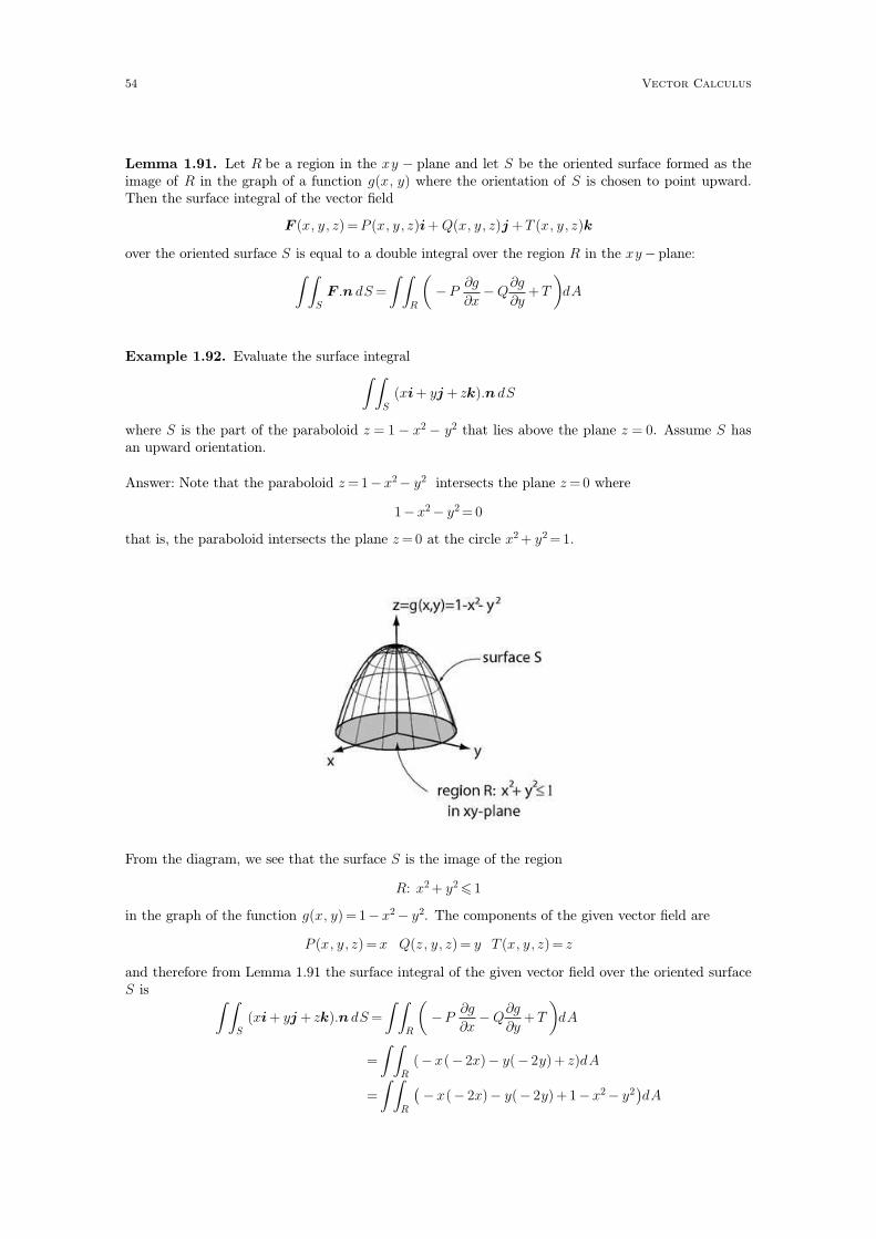
Lemma 1.91. Let R be a region in the xy − plane and let S be the oriented surface formed as theimage of R in the graph of a function g(x, y) where the orientation of S is chosen to point upward.Then the surface integral of the vector field
F (x, y, z) =P (x, y, z)i+ Q(x, y, z)j +T (x, y, z)k
over the oriented surface S is equal to a double integral over the region R in the xy − plane:
∫ ∫
S
F .n dS =
∫ ∫
R
(
−P∂g
∂x−Q
∂g
∂y+T
)
dA
Example 1.92. Evaluate the surface integral∫ ∫
S
(xi + yj + zk).n dS
where S is the part of the paraboloid z = 1 − x2 − y2 that lies above the plane z = 0. Assume S hasan upward orientation.
Answer: Note that the paraboloid z =1− x2− y2 intersects the plane z =0 where
1− x2− y2 = 0
that is, the paraboloid intersects the plane z =0 at the circle x2 + y2 =1.
From the diagram, we see that the surface S is the image of the region
R: x2 + y2 6 1
in the graph of the function g(x, y) = 1− x2− y2. The components of the given vector field are
P (x, y, z)= x Q(z, y, z) = y T (x, y, z)= z
and therefore from Lemma 1.91 the surface integral of the given vector field over the oriented surfaceS is
∫ ∫
S
(xi + yj + zk).n dS =
∫ ∫
R
(
−P∂g
∂x− Q
∂g
∂y+ T
)
dA
=
∫ ∫
R
(− x(− 2x)− y(− 2y)+ z)dA
=
∫ ∫
R
(
− x(− 2x)− y(− 2y) + 1− x2− y2)
dA
54 Vector Calculus

because z = 1−x2− y2. Hence∫ ∫
S
(xi+ yj + zk).n dS =
∫ ∫
R
(
1 +x2 + y2)
dA
where the region R is the unit disc
and so we convert to polar coordinates
∫ ∫
S
(xi + yj + zk).n dS =
∫ ∫
R
(
1 + x2 + y2)
dA
=
∫
0
2π ∫
0
1(
1 + r2cos2θ + r2sin2θ)
rdrdθ
=
∫
0
2π( ∫
0
1
(1 + r2)rdr
)
dθ
=
∫
0
2π(
[
r2
2+
r4
4
]
0
1)
dθ
=
∫
0
2π 3
4dθ
=3π
2.
1.6 Surface integrals 55

1.7 Triple integrals and Divergence theorem
1.7.1 Triple integrals
Definition 1.93. Let B be a rectangular box in three dimension defined by
B = {(x, y, z)| a6 x6 b, c 6 y 6 d, r 6 z 6 s}.Divide the rectangular box B into suboxes by partitioning the intervals a 6 x 6 b , c 6 y 6 d and r 6
z 6 s:
a =x0 <x1 <� <xm = b
c = y0 < y1 <� < yn = d
r = z0 < z1 <� < zl = s
and define the subbox Bijk as
Bijk = {(x, y, z)|xi−1 6 x 6xi , yj−1 6 y 6 yj , zk−1 6 y 6 zk}
Choose points (xijk∗ , yijk
∗ , zijk∗ ) in each subbox Bijk. Let ∆Vijk denote the volume of the subrectangle
Bijk and let∥
∥P∥
∥ denote the length of the longest diagonal of all subboxes (note that as we take
smaller subboxes of B we have that∥
∥P∥
∥→ 0). Then the triple integral of the function f(x, y, z)
over the rectangular box B is defined to be the limit
∫ ∫ ∫
B
f(x, y, z)dV = lim‖P ‖→0
∑
i=1
m∑
j=1
n∑
k=1
l
f(xijk∗ , yijk
∗ , zijk∗ )∆Vijk
if this limit exists.
The above definition is not usually used to evaluate triple integrals. The method of evaluating tripleintegrals over rectangular boxes is based on the following theorem.
Theorem 1.94. (Fubini’s Theorem for triple integrals) If the function f(x, y, z) is continuousat each point in a rectangular box
B = {(x, y)| a6 x6 b, c 6 y 6 d, r 6 z 6 s}then
∫ ∫ ∫
B
f(x, y, z)dV =
∫
a
b ∫
c
d ∫
r
s
f(x, y, z)dz dy dx. (1.16)
From the above theorem we see that the evaluation of a triple integral requires two instances of par-tial integration.
56 Vector Calculus

Example 1.95. Evaluate the triple integral∫ ∫ ∫
B
xyz2 dV
where B is the rectangular box
B = {(x, y, z)| 06 x6 1,− 16 y 6 2, 0 6 z 6 3}.
Answer: By Fubini’s Theorem for triple integrals
∫ ∫ ∫
B
xyz2 dV =
∫
0
1 ∫
−1
2 ∫
0
3
xyz2 dz dy dx
=
∫
0
1 ∫
−1
2( ∫
0
3
xyz2 dz
)
dy dx
=
∫
0
1 ∫
−1
2[
xyz3
3
]
z=0
z=3
dy dx
=
∫
0
1 ∫
−1
2
9xy dy dx
=
∫
0
1[
9xy2
2
]
y=−1
y=2
dx
=
∫
0
1 27x
2dx
=
[
27x2
4
]
0
1
=27
4
We also wish to evaluate triple integrals over cylindrical solids that are centered around the z − axis.The following diagram illustrates the solid
V = {(x, y, z)|x2 + y2 6 a2, m 6 z 6 l }
that is bounded by the cylinder x2 + y2 6 a2 and the horizontal planes z = l, z =m.
If we use the tranformationx = r cosθy = r sin θ
z = z
then the set V can be rewritten in cylindrical coordinates (r, θ, z)
V = {(r, θ, z)|06 r 6 a, 06 θ 6 2π, m 6 z 6 l}.
1.7 Triple integrals and Divergence theorem 57

Theorem 1.96. If the function f(x, y, z) is continuous at each point in a cylindrical solid
V = {(x, y, z)|x2 + y2 6 a2, m 6 z 6 l }
then by converting to cylindrical coordinates∫ ∫ ∫
V
f(x, y, z)dV =
∫
0
2π ∫
0
a ∫
m
l
f(r cosθ, r sinθ, z)rdz dr dθ.
1.7.2 Divergence theorem
Theorem 1.97. (Divergence theorem) Let E be a solid region whose boundary surface S has aoutward orientation. Let F be a vector field whose component functions have continuous partialderivatives on an open region that contains E. Then
∫ ∫
S
F .n dS =
∫ ∫ ∫
E
div(F )dV
Note that the Divergence theorem states that a surface integral over a surface S that encloses a solidregion E may be obtained by evaluating a triple integral the solid E. We illustrate the Divergencetheorem by the following examples.
Example 1.98. Verify the Divergence theorem for the vector field F
F (x, y, z) = 3xi +xyj + 2xzk
and the solid region E that is the cube bounded by the six planes
x =0 y = 0 z = 0x =1 y =1 z = 1.
Answer: We evaluate the surface integral∫ ∫
S
(3xi+xyj +2xzk).n ds
and the triple integral∫ ∫ ∫
E
div(3xi+ xyj +2xzk)dV .
and verify that these are equal. The solid cube E
has boundary surface S consisting of the six truncated planes S1, S2, S3, S4, S5 and S6
58 Vector Calculus

Figure 1.11.
and each of these six planes has an orientation that points out of the solid E.
We first evaluate the triple integral
∫ ∫ ∫
E
div(3xi +xyj +2xzk)dV =
∫ ∫ ∫
E
(
∂
∂x(3x)+
∂
∂y(xy)+
∂
∂z(2xz)
)
dV
=
∫ ∫ ∫
E
(3 +x +2x) dV
=
∫
0
1 ∫
0
1 ∫
0
1
(3 + 3x) dzdydx (by Theorem 1.94)
=
∫
0
1 ∫
0
1 (
[3z +3xz]z=0z=1
)
dydx
=
∫
0
1 ∫
0
1
(3 +3x)dydx
=
∫
0
1 (
[3y +3xy]y=0y=1
)
dx
=
∫
0
1
(3 +3x) dx
=
[
3x+3x2
2
]
x=0
x=1
=9
2
Next we evaluate the surface integral of F over S. As the surface S consists of S1, S2, S3, S4,
S5 and S6 we have∫ ∫
S
F .n dS =
∫ ∫
S1
F .n dS +
∫ ∫
S2
F .n dS +
∫ ∫
S3
F .n dS
+
∫ ∫
S4
F .n dS +
∫ ∫
S5
F .n dS +
∫ ∫
S6
F .n dSs(1.17)
and each∫ ∫
SiF .n dS on the right hand side of (1.17) is evaluated by first expressing Si as para-
metric surface r(u, v) and then using the definition of a surface integral∫ ∫
Si
F .n dS=
∫ ∫
R
F (x(u, v), y(u, v), z(u, v)).(ru ×rv) dA. (1.18)
Note that we should choose each parametrization r(u, v) of Si such that the normal vector ru × rv
has the same direction with the outward normal vector of Si as shown in Figure 1.11 (if the normal
vector ru × rv is in the opposite direction of the outward normal vector of Si then∫ ∫
SiF .n ds on
the right hand side of (1.17) should be adjusted by a minus sign).
1.7 Triple integrals and Divergence theorem 59

S1
A parametrization for S1 is
r(u, v)= vi+ j + uk (u, v)∈R
where R is the rectangular region
Figure 1.12.
The vectors ru and rv are
ru =∂x
∂ui +
∂y
∂uj +
∂z
∂uk =0i+0j +k
rv =∂x
∂vi+
∂y
∂vj +
∂z
∂vk = i+0j +0k
andru×rv =k × i
=
∣
∣
∣
∣
∣
∣
i j k
0 0 11 0 0
∣
∣
∣
∣
∣
∣
= j.
Notice that the normal vector ru × rv = j points in the the same direction with the outward normalvector of S1 as shown in Figure 1.11. Using (1.18)
∫ ∫
S1
(3xi +xyj +2xzk).n dS =
∫ ∫
R
(3vi + vj +2uvk).(ru× rv) dA
=
∫ ∫
R
(3vi + vj +2uvk).(j) dA
=
∫ ∫
R
v dA
=
∫
0
1 ∫
0
1
v dv du (by Theorem 1.61)
=
∫
0
1[
v2
2
]
0
1
du
=
∫
0
1 1
2du
=1
2
and therefore∫ ∫
S1
F .n dS =1
2
60 Vector Calculus

S2
A parametrization for S2 is
r(u, v)= ui+ 0j + vk (u, v)∈R (1.19)
where R is the rectangular region shown in Figure 1.12. Notice the difference with the parametriza-tion for S1 – the i and k components are exchanged. This causes the normal vector ru × rv to pointin the opposite direction
ru =∂x
∂ui +
∂y
∂uj +
∂z
∂uk = i+0j +0k
rv =∂x
∂vi+
∂y
∂vj +
∂z
∂vk = 0i+0j +k
and
ru×rv = i×k
=
∣
∣
∣
∣
∣
∣
i j k
1 0 00 0 1
∣
∣
∣
∣
∣
∣
=− j.
The parametrization (1.19) is chosen so that the normal vector ru × rv = − j points in the the samedirection with the outward normal vector of S2 as shown in Figure 1.11. Using (1.18)
∫ ∫
S2
(3xi+ xyj + 2xzk).n dS =
∫ ∫
R
(3ui+0j +2uvk).(ru× rv) dA
=
∫ ∫
R
(3ui+0j +2uvk).(− j) dA
=
∫ ∫
R
0 dA
=
∫
0
1 ∫
0
1
0 dv du
= 0and therefore
∫ ∫
S2
F .n dS = 0
S3
A parametrization for S3 is
r(u, v)= i+uj + vk (u, v)∈R
where R is the rectangular region shown in Figure 1.12. The vectors ru and rv are
ru =∂x
∂ui +
∂y
∂uj +
∂z
∂uk =0i+ j +0k
rv =∂x
∂vi+
∂y
∂vj +
∂z
∂vk = 0i+0j +k
and
ru×rv = j ×k
=
∣
∣
∣
∣
∣
∣
i j k
0 1 00 0 1
∣
∣
∣
∣
∣
∣
= i.
1.7 Triple integrals and Divergence theorem 61

The surface integral is
∫ ∫
S3
(3xi+ xyj + 2xzk).n dS =
∫ ∫
R
(3i +uj +2vk).(ru× rv) dA
=
∫ ∫
R
(3i +uj +2vk).(i) dA
=
∫ ∫
R
3 dA
=
∫
0
1 ∫
0
1
3 dv du
= 3and therefore
∫ ∫
S3
F .n dS = 3
S4
A parametrization for S4 is
r(u, v)= 0i+ vj + uk (u, v)∈R
where R is the rectangular region shown in Figure 1.12. The vectors ru and rv are
ru =∂x
∂ui +
∂y
∂uj +
∂z
∂uk =0i+0j +k
rv =∂x
∂vi+
∂y
∂vj +
∂z
∂vk = 0i+ j +0k
and
ru×rv = i×k
=
∣
∣
∣
∣
∣
∣
i j k
0 0 10 1 0
∣
∣
∣
∣
∣
∣
=− i.
The surface integral is
∫ ∫
S4
(3xi+ xyj + 2xzk).n dS =
∫ ∫
R
(0i +0j +0k).(ru× rv) dA
=
∫ ∫
R
(0i +0j +0k).(− i) dA
=
∫ ∫
R
0 dA
=
∫
0
1 ∫
0
1
0 dv du
= 0and therefore
∫ ∫
S4
F .n dS = 0
S5
A parametrization for S5 is
r(u, v)= ui+ vj +1k (u, v)∈R
where R is the rectangular region shown in Figure 1.12. The vectors ru and rv are
ru =∂x
∂ui +
∂y
∂uj +
∂z
∂uk = i+0j +0k
rv =∂x
∂vi+
∂y
∂vj +
∂z
∂vk = 0i+ j +0k
62 Vector Calculus

and
ru×rv = i× j
=
∣
∣
∣
∣
∣
∣
i j k
1 0 00 1 0
∣
∣
∣
∣
∣
∣
= k.
The surface integral is
∫ ∫
S5
(3xi +xyj +2xzk).n dS =
∫ ∫
R
(3ui+ uvj +2uk).(ru×rv) dA
=
∫ ∫
R
(3ui+ uvj +2uk).(k) dA
=
∫ ∫
R
2u dA
=
∫
0
1 ∫
0
1
2u dv du
= 1and therefore
∫ ∫
S5
F .n dS = 1
S6
A parametrization for S6 is
r(u, v)= vi+ uj +0k (u, v)∈R
where R is the rectangular region shown in Figure 1.12. The vectors ru and rv are
ru =∂x
∂ui +
∂y
∂uj +
∂z
∂uk =0i+ j +0k
rv =∂x
∂vi+
∂y
∂vj +
∂z
∂vk = i+0j +0k
and
ru×rv = j × i
=
∣
∣
∣
∣
∣
∣
i j k
0 1 01 0 0
∣
∣
∣
∣
∣
∣
=−k.
The surface integral is
∫ ∫
S6
(3xi +xyj +2xzk).n dS =
∫ ∫
R
(3vi +uvj + 0k).(ru ×rv) dA
=
∫ ∫
R
(3vi +uvj + 0k).(−k) dA
=
∫ ∫
R
0 dA
=
∫
0
1 ∫
0
1
0 dv du
=0and therefore
∫ ∫
S6
F .n dS = 0
1.7 Triple integrals and Divergence theorem 63

So we have∫ ∫
S
F .n dS =
∫ ∫
S1
F .n dS +
∫ ∫
S2
F .n dS +
∫ ∫
S3
F .n dS
+
∫ ∫
S4
F .n dS +
∫ ∫
S5
F .n dS +
∫ ∫
S6
F .n dS
=1
2+ 0 +3 + 0 +1 + 0
=9
2.
Hence we have∫ ∫
S
F .n dS =
∫ ∫ ∫
E
div(F )dV =9
2
which verifies the Divergence theorem.
One application of the Divergence theorem is in the evaluation of surface integrals∫ ∫
SF .n dS
where S is the boundary surface of a solid region E. As we saw in the previous example, the evalua-tion of such surface integrals can be tedious. It is sometimes easier to calculate the correspondingtriple integral
∫ ∫ ∫
Ediv(F )dV ; by the Divergence theorem
∫ ∫
S
F .n dS =
∫ ∫ ∫
E
div(F )dV
this gives the answer of the required surface integral.
Example 1.99. Use the Divergence Theorem to evaluate the surface integral
∫ ∫
S
(yezi+ y2j + cos (xy)k).n dS
where S is the surface of the solid bounded by the cylinder x2 + y2 = 9 and the planes z = 0 and z =2.
Answer: The closed cylinder S below
encloses the solid region
E = {(x, y, z)|x2 + y2≤ 9 and 0≤ z ≤ 2}
From the Divergence Theorem∫ ∫
S
F .ndS =
∫ ∫ ∫
E
divF dV
64 Vector Calculus

we have that our required surface integral I can be expressed as a triple integral
I =
∫ ∫
S
(yezi+ y2j + cos(xy)k).n dS =
∫ ∫ ∫
E
(
∂
∂x(yez)+
∂
∂y(y2)+
∂
∂z(cos(xy))
)
dxdy dz
=
∫ ∫ ∫
E
2y dxdy dz
From Theorem 1.96 we can convert to cylindrical coordinates
I =
∫ ∫ ∫
E
2y dxdy dz
=
∫
0
2π ∫
0
3 ∫
0
2
2r sinθ r dzdrdθ
=
∫
0
2π ∫
0
3[
2r2sinθz]
z=0
z=2drdθ
=
∫
0
2π ∫
0
3
4r2sinθdrdθ
=
∫
0
2π[
4r3sinθ
3
]
r=0
r=3
dθ
=
∫
0
2π
36 sinθdθ
=0and so the surface integral
∫ ∫
S
(yezi+ y2j + cos(xy)k).n dS = 0.
1.7 Triple integrals and Divergence theorem 65

Chapter 2
Laplace transforms
The Laplace transform changes a function y(t) in the t variable to a corresponding function Y (s) inthe new independent variable s.
The Laplace transform provides a method of solving differential and integral equations by convertingthese to algebraic expressions as we shall see in the following sections.
2.1 Definition and existence of Laplace transforms
2.1.1 Improper integrals
Recall that a definite integral has two finite limits of integration
∫
a
b
f(t)dt.
If we require that one of these limits of integration be ∞ then we need an improper integral –
Definition 2.1. The improper integral
∫
a
∞g(t)dt (2.1)
is defined as the limit∫
a
∞g(t)dt= lim
R→∞
∫
a
R
g(t)dt. (2.2)
The improper integral (2.1) is said to converge if the limit of (2.2) exists and is finite. Otherwisethe improper integral is said to diverge.
Example 2.2. Determine if the following improper integrals converge or diverge
i.∫
1
∞e −t dt
ii.∫
1
∞et dt
Answer:
i.∫
1
∞e −t dt=limR→∞
∫
1
Re−t dt
=limR→∞
[
e−t
− 1
]
1
R
=limR→∞(
e−1− e−R)
=limR→∞ e−1− limR→∞ e−R
= e−1− limR→∞ e−R (as e−1 is a constant)
=e−1 (e−R→ 0 as R→∞)
67

and therefore∫
1
∞e −t dt converges. Note by defintion of the improper integral
∫
1
∞e −t dt =e−1.
ii.∫
1
∞e t dt=limR→∞
∫
1
Ret dt
=limR→∞[
et]
1
R
=limR→∞(
eR − e)
=limR→∞ eR − limR→∞ e
=(
limR→∞ eR)
− e (as e is a constant)
=∞ (eR→∞ as R→∞)
and therefore∫
1
∞e t dt diverges.
The shaded areas of the graphs below represent the integrals of∫
1
∞e −t dt and
∫
1
∞e t dt respec-
tively. Notice that the shaded area in the both graphs increase as t increases, however the rate atwhich the area in the first graph increases is much smaller than the rate at which the area in thesecond graph increases. This should suggest that
∫
1
∞e t dt diverges.
Figure 2.1.
Notice in the above graph that e−t tends to zero as t gets larger, in other words
limt→∞
e−t = 0,
also notice that et does not tend to zero as t gets larger
limt→∞
et =∞.
From Example 2.2 we saw that∫
1
∞e−tdt converges and
∫
1
∞etdt diverges. Therefore it would
seem that if
limt→∞
g(t)=∞then
∫
a
∞g(t)dt
diverges. This is in fact the case, we state this fact formally:
Lemma 2.3. If limt→∞ g(t)=∞ then the improper integral∫
a
∞g(t)dt diverges.
68 Laplace transforms

Proof. (Not required). The limt→∞ g(t) is ∞ if, by definition, given any K > 0 there exists a t −value t0 such that g(t) >K for all t > t0. Fix such a K and t0. Then
limR→∞
∫
a
R
g(t)dt= limR→∞
(
∫
a
t0
g(t)dt+
∫
t0
R
g(t)dt
)
=
∫
a
t0
g(t)dt + limR→∞
∫
t0
R
g(t)dt
>
∫
a
t0
g(t)dt + limR→∞
∫
t0
R
Kdt because g(t) >K
=
∫
a
t0
g(t)dt+ limR→∞
(KR−Kt0)
=∞
and hence∫
a
∞g(t)dt diverges.
�
2.1.2 Definition and examples of Laplace tranform
Definition 2.4. The Laplace transform of the function y(t), denoted by L[y(t)], is
L[y(t)]=
∫
0
∞e −sty(t)dt (2.3)
and is defined for those values of s for which the improper integral (2.3) converges. Note that L[y(t)]is a function of s and we denote
L[y(t)] =Y (s).
Example 2.5. Use the definition of the Laplace transform to determine L[ekt]where k is a real con-stant.
L[ekt] =
∫
0
∞e −st ektdt
=
∫
0
∞e −(s−k )t dt
= limR→∞
∫
0
R
e −(s−k )t dt
(2.4)
and when s = k we have
limR→∞
∫
0
R
e −(s−k )t dt = limR→∞
∫
0
R
1dt
= limR→∞
R
= ∞
(2.5)
and therefore L[ekt] does not exist for s = k. Now consider when s� k
limR→∞
∫
0
R
e −(s−k )t dt= limR→∞
[
e −(s−k )t
− (s− k)
]
0
R
= limR→∞
(
1
s− k− e −(s−k )R
s− k
)
=1
s− k− lim
R→∞
e −(s−k )R
s− k
2.1 Definition and existence of Laplace transforms 69

From the graphs of Figure 2.1 we see that
limR→∞
e−R = 0 and limR→∞
eR =∞and in general
limR→∞
eaR =
{
0 if a< 0∞ if a > 0
(2.6)
that is, limR→∞ e aR depends only on the sign of a. Hence
limR→∞
e −(s−k )R =
{
0 if − (s− k)< 0∞ if − (s− k)> 0
(2.7)
and therefore
L[ekt] =1
s− k− lim
R→∞
e −(s−k )R
s− k
=1
s− k−(
1
s− k
)
limR→∞
e −(s−k )R(2.8)
and from (2.7) the limit in (2.8) is zero only when s > k. So we have
L[ekt] =1
s− k(2.9)
and this holds only when s >k.
Note by setting k =0 in (2.9) we get
L[1]=1
swhen s > 0. (2.10)
Example 2.6. Use the definition of the Laplace transform to show that
L[sinkt] =k
s2 + k2
when s > 0.
Answer:
L[sin kt] =
∫
0
∞e −st sin ktdt
= limR→∞
∫
0
R
e −st sin kt dt.
Using the integration by parts formula∫
a
b
v du = [uv]ab −∫
a
b
u dv
withv = sin kt du = e−st dt
dv = k coskt dt u=− e−st
sgives
∫
0
R
e −st sin kt dt=−[
e−stsinkt
s
]
0
R
+k
s
∫
0
R
e −st coskt dt (2.11)
Integrate∫
0
Re −st cos kt by parts again with
v = coskt du = e−st dt
dv =− k sin kt dt u =− e−st
sto get
∫
0
R
e −st cos kt dt=−[
e−stcos kt
s
]
0
R
− k
s
∫
0
R
e −st sinkt dt. (2.12)
70 Laplace transforms

Substituting (2.12) into (2.11) gives
∫
0
R
e −st sinkt dt=−[
e−stsin kt
s
]
0
R
− k
s
[
e−stcos kt
s
]
0
R
− k2
s2
∫
0
R
e −st sin kt dt. (2.13)
and solving for∫
0
Re −st sinkt dt in (2.13) gives
s2 + k2
s2
∫
0
R
e −st sin kt dt=− 1
s
[
e−stsinkt]
0
R − k
s2
[
e−stcos kt]
0
R(2.14)
and evaluating the right side of (2.14) using the limits of integration gives
s2 + k2
s2
∫
0
R
e −st sin kt dt=− 1
se−sRsin kR − k
s2e−sRcos kR +
k
s2(2.15)
and taking the limit limR→∞ of both sides of (2.15) we have
s2 + k2
s2lim
R→∞
(
∫
0
R
e −st sin kt dt
)
= limR→∞
(
− 1
se−sRsin kR − k
s2e−sRcoskR +
k
s2
)
. (2.16)
Notice as − 16 sinkR 6 1 implies that
− e−sR 6 e−sRsin kR 6 e−sR
and taking limits gives
− limR→∞
e−sR 6 limR→∞
(
e−sRsinkR)
6 limR→∞
e−sR (2.17)
Now from equation (2.6) above if s > 0 (and only if s > 0) then
limR→∞
e−sR =0.
So when s > 0 the inequality (2.17) simplifies to
0 6 limR→∞
(
e−sRsin kR)
6 0
and therefore
limR→∞
e−sRsin kR =0 . (2.18)
Similarly one can show when s > 0 that
limR→∞
e−sRcos kR =0, (2.19)
and substituting (2.18) and (2.19) into the right side of (2.16) we have
s2 + k2
s2lim
R→∞
(
∫
0
R
e −st sin kt dt
)
=k
s2
⇒ limR→∞
(
∫
0
R
e −st sin kt dt
)
=k
s2 + k2
⇒ L[sin kt] =k
s2 + k2
when s > 0.
Example 2.7. Use the definition of the Laplace transform to show that when n =0, 1, 2,�L[tn] =
n!
sn+1(2.20)
when s > 0.
2.1 Definition and existence of Laplace transforms 71

Answer: From (2.10) we know that
L[1]=1
swhen s > 0
⇒L[t0] =0!
s0+1when s > 0
and so (2.20) holds when n = 0. We therefore need to consider when n =1, 2, 3,�L[tn] =
∫
0
∞e −st tn dt
= limR→∞
∫
0
R
e −st tn dt.
Using the integration by parts formula with
v = tn du = e−st dt
dv =ntn−1 dt u =− e−st
sgives
∫
0
R
e −st tn dt=−[
e−sttn
s
]
0
R
+n
s
∫
0
R
e −st tn−1 dt. (2.21)
Taking the limit limR→∞ of both sides of (2.21) we have
limR→∞
(
∫
0
R
e −st tn dt
)
= limR→∞
(
−[
e−sttn
s
]
0
R)
+n
slim
R→∞
(
∫
0
R
e −st tn−1 dt
)
and by using the definition of the Laplace transforms L[tn] and L[tn−1] we have
L[tn]= limR→∞
(
−[
e−sttn
s
]
0
R)
+n
sL[tn−1]. (2.22)
Now
limR→∞
(
−[
e−sttn
s
]
0
R)
= limR→∞
(
− e−sRRn
s
)
= limR→∞
(
− Rn
sesR
)
and this limit is of the indeterminate form∞∞ . Applying L’Hospitals rule by differentiating the
numerator and denominator n times with respect to R, we have
limR→∞
(
− Rn
sesR
)
= limR→∞
− n!
sn+1esR
= 0 when s > 0and therefore
limR→∞
(
−[
e−sttn
s
]
0
R)
=0 when s > 0 . (2.23)
Substituting (2.23) into (2.22) gives the formula
L[tn]=n
sL[tn−1] valid for n =1, 2, 3,� and s > 0. (2.24)
Notice that by replacing n by n− 1 in (2.24) we have
L[tn−1]=n− 1
sL[tn−2] (2.25)
72 Laplace transforms

and similarly by replacing n with n− 2, n− 3,� , 2, 1 in (2.24) we have, respectively,
L[tn−2]=n− 2
sL[tn−3]
L[tn−3]=n− 3
sL[tn−4]
L[t2]=2
sL[t1]
L[t]=1
sL[t0]
(2.26)
Finally we get (2.20) by using the equations (2.25) and (2.26) to express L[tn] in terms of L[t0] =
L[1] =1
s:
L[tn]=n
sL[tn−1] from (2.24)
=n
s
(
n− 1
sL[tn−2]
)
from (2.25)
=n
s
n− 1
s
(
n− 2
sL[tn−3]
)=
n
s
n− 1
s
n− 2
s� 2
sL[t1]
=n
s
n− 1
s
n− 2
s� 2
s
1
sL[t0]
=n!
snL[t0]
=n!
sn+1
which is our desired result.
2.1.3 Existence of Laplace transform
In Examples 2.5, 2.6 and 2.7 we were able to determine the Laplace transforms of the functions ekt ,sin kt and tn respectively. We also showed that the Laplace tranforms of those functions existed foronly certain value of s:
y(t) L[y(t)] Laplace tranform existswhen
ekt 1
s− ks >k
sin ktk
s2 + k2s > 0
tnn!
sn+1s > 0
We now give an example of a function that does not have a Laplace tranform for any value of s.
Example 2.8. Show that the Laplace transform of et2does not exist for any real value of s.
Answer: Recall that from Definition 2.4 L[et2], given by:
L[et2] =
∫
0
∞e −stet2dt (2.27)
is defined only for those values of s for which the improper integral on the right converges. Fix anyvalue of s. If we can show that for this value of s
limt→∞
e −stet2 =∞
2.1 Definition and existence of Laplace transforms 73
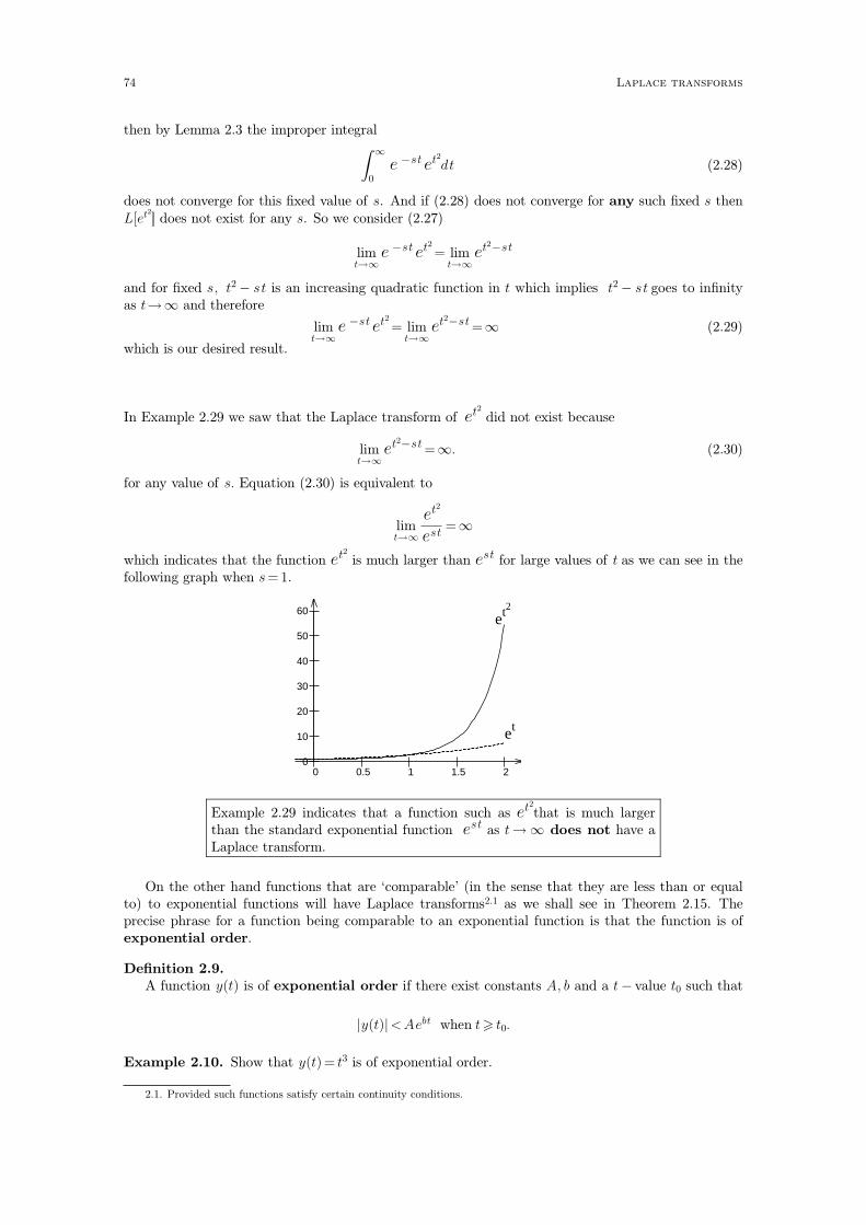
then by Lemma 2.3 the improper integral∫
0
∞e −stet2dt (2.28)
does not converge for this fixed value of s. And if (2.28) does not converge for any such fixed s thenL[et2] does not exist for any s. So we consider (2.27)
limt→∞
e −stet2 = limt→∞
et2−st
and for fixed s, t2 − st is an increasing quadratic function in t which implies t2 − st goes to infinityas t→∞ and therefore
limt→∞
e −stet2 = limt→∞
et2−st =∞ (2.29)
which is our desired result.
In Example 2.29 we saw that the Laplace transform of et2 did not exist because
limt→∞
et2−st =∞. (2.30)
for any value of s. Equation (2.30) is equivalent to
limt→∞
et2
est=∞
which indicates that the function et2 is much larger than est for large values of t as we can see in thefollowing graph when s =1.
0
10
20
30
40
50
60
0 0.5 1 1.5 2
et
et2
Example 2.29 indicates that a function such as et2that is much largerthan the standard exponential function est as t→∞ does not have aLaplace transform.
On the other hand functions that are ‘comparable’ (in the sense that they are less than or equalto) to exponential functions will have Laplace transforms2.1 as we shall see in Theorem 2.15. Theprecise phrase for a function being comparable to an exponential function is that the function is ofexponential order.
Definition 2.9.A function y(t) is of exponential order if there exist constants A, b and a t− value t0 such that
|y(t)|<Aebt when t> t0.
Example 2.10. Show that y(t)= t3 is of exponential order.
2.1. Provided such functions satisfy certain continuity conditions.
74 Laplace transforms
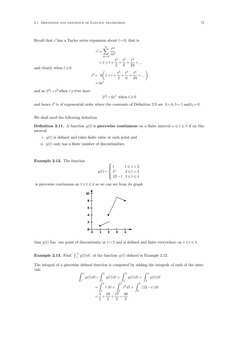
Recall that et has a Taylor series expansion about t=0, that is
et =∑
m=0
∞tm
m!
= 1 + t+t2
2+
t3
6+
t4
24+�
and clearly when t> 0
t3 < 6
(
1 + t+t2
2+
t3
6+
t4
24+� )
=6et
and as |t3|= t3when t> 0we have
|t3|< 6et when t> 0
and hence t3 is of exponential order where the constants of Definition 2.9 are A =6, b=1 and t0 =0.
We shall need the following definition
Definition 2.11. A function y(t) is piecewise continuous on a finite interval a 6 t 6 b if on thisinterval
i. y(t) is defined and takes finite value at each point and
ii. y(t) only has a finite number of discontinuities.
Example 2.12. The function
y(t)=
t 16 t < 2
t2 26 t < 312− t 3 6 t6 4
is piecewise continuous on 16 t6 4 as we can see from its graph
0
2
4
6
8
10
0 1 2 3 4 0
2
4
6
8
10
0 1 2 3 4 0
2
4
6
8
10
0 1 2 3 4 0
2
4
6
8
10
0 1 2 3 4 0
2
4
6
8
10
0 1 2 3 4
that y(t) has one point of discontinuity at t=2 and is defined and finite everywhere on 16 t6 4.
Example 2.13. Find∫
1
4y(t)dt of the function y(t) defined in Example 2.12.
The integral of a piecewise defined function is computed by adding the integrals of each of the inter-vals
∫
1
4
y(t)dt=
∫
1
2
y(t)dt +
∫
2
3
y(t)dt+
∫
3
4
y(t)dt
=
∫
1
2
t dt+
∫
2
3
t2 dt+
∫
3
4
(12− t )dt
=3
2+
19
3+
17
2=
49
3
2.1 Definition and existence of Laplace transforms 75

To find the Laplace transform of a piecewise defined function y(t) such as the one defined inExample 2.12, we use the same procedure of adding the integral over each interval as done inExample 2.13 :
Example 2.14. Sketch the graph of the following function
y(t) =
0 06 t < 1t 16 t< 20 t> 2
and determine L[y(t)].
Answer: The graph of y(t) is
0
1
2
3
4
21 0
1
2
3
4
21 0
1
2
3
4
21 0
1
2
3
4
21 0
1
2
3
4
21
By definition
L[y(t)]=
∫
0
∞e −sty(t)dt
Now as y(t) is a piecewise-defined defined function, it follows that e −sty(t) is also piecewise-defined:
e −sty(t)=
0 0 6 t< 1
e −stt 16 t < 20 t> 2
and∫
0
∞e −sty(t)dt=
∫
0
1
e −sty(t)dt+
∫
1
2
e −sty(t)dt+
∫
2
∞e −sty(t)dt
=
∫
0
1
0dt+
∫
1
2
e −sty(t)dt+
∫
2
∞0 dt
= 0 +
∫
1
2
e −sttdt+ 0
=
∫
1
2
e −sttdt
and using integration by parts with
v = t du = e−st dt
dv = 1 dt u =− e−st
swe have
∫
1
2
e −stt dt=
[
− e−st t
s
]
1
2
+1
s
∫
1
2
e −st dt
=
[
− e−st t
s
]
1
2
+
[
− e−st
s2
]
1
2
=
(
1
s2+
1
s
)
e−s −(
1
s2+
2
s
)
e−2s
and therefore
L[y(t)] =
(
1
s2+
1
s
)
e−s −(
1
s2+
2
s
)
e−2s .
76 Laplace transforms

We now state a theorem that guarantees the existence of the Laplace transform of functions that areof exponential order and that are piecewise continuous.
Theorem 2.15. (Existence) Let y(t) be a function such that |y(t)|<Aebt when t > t0 for someconstants A, b and t0 (that is, y(t) is of exponential order). Also let y(t) be piecewise continuous onany finite interval c1 6 t6 c2 where c1, c2 > 0. Then the Laplace transform of y(t) exists for s > b.
Proof. Not required. �
Example 2.16. Show that the following functions are of exponential order and hence use Theorem2.15 to prove that their Laplace transforms exist.2.2
i. e5t
ii. sin 2t
iii. y(t) =
0 06 t < 1t 1 6 t < 20 t> 2
Answer:
i. |e5t|<1.e5t for t > 0 and so the constants of Definition 2.9 are A = 1, b = 5 and t0 = 0. e5t is afunction that is continuous everywhere (see the graph on Figure 2.1) and is hence continuouson every finite interval and is therefore piecewise continuous on every finite interval . So by
Theorem 2.15 the Laplace transform of e5t exists for s > 5, a fact we already know fromExample 2.5.
ii. |sin 2t|< 2 = 2e0t for t > 0 and so A = 2, b = 0 and t0 = 0. sin 2t is continuous everywhere and istherefore piecewise continuous on every finite interval. So by Theorem 2.15 the Laplace trans-form of sin 2t exists for s > 0, which we already know from Example 2.6.
iii. From the graph of y(t) in Example 2.14 we see that |y(t)| < 2 for t > 0 and therefore |y(t)| <2 = 2e0t for t > 0 and so A = 2, b = 0 and t0 = 0. If we consider any finite interval c1 6 t 6 c2
where c1, c2 > 0 then y(t) has at most two points of discontinuity in the interval c1 6 t 6 c2
depending on whether or not x = 1, 2 lie in the interval c1 6 t 6 c2. Hence y(t) is piecewise con-tinuous on every finite interval. By Theorem 2.15 the Laplace transform of y(t) exists for s >
0.
Remark 2.17. It is possible to obtain the Laplace transform of functions that do not satify the
hypotheses of Theorem 2.15, for example1
t√ 2.3 and the Dirac delta ‘function’ considered later. The
main use of Theorem 2.15 is to guarantee the existence of the Laplace transform of standard func-tions such as ekt, cos kt, sinh kt, t5 + 4t3 − 3t + 1 and piecewise functions such as those in Examples2.12 and 2.14.
2.2. Assume that we do not know the Laplace transforms of these functions have not been determined in Examples 2.5,2.6 and 2.14. Note we do not actually find Laplace transforms by Theorem 2.15, we just show that the transform exists.
2.3. See Kreyszig [2] Section 6.1
2.1 Definition and existence of Laplace transforms 77
2.2 Properties of Laplace transforms
2.2.1 Linearity property
The Laplace transform has the linearity property
Theorem 2.18. Let y1(t) and y2(t) be functions whose Laplace transforms exist and let c1 and c2 bescalars. Then
L[c1y1(t)+ c2y2(t)]= c1L[y1(t)] + c2L[y2(t)].
Proof. Using the definition of the Laplace transform
L[c1y1(t)+ c2y2(t)]=
∫
0
∞e−st
(
c1y1(t) + c2y2
)
dt
= c1
∫
0
∞e−sty1(t)dt + c2
∫
0
∞e−sty1(t)dt
= c1L[y1(t)]+ c2L[y2(t)]�
Example 2.19. Use the linearity property of the Laplace transform to determine
i. L[t2 +3t+2]
ii. L[cosh kt]wherek is a real constant.
Answer:
i.L[t2 +3t+2] =L[t2] + 3L[t] + 2L[1]
=2
s3+3
(
1
s2
)
+2
(
1
s
)
=2
s3+
3
s2+
2
s
ii. By definition cosh kt=e−kt + ekt
2therefore
L[cosh kt] = L
[
e−kt + ekt
2
]
=1
2L[e−kt] +
1
2L[ekt]
=1
2
(
1
s + k
)
+1
2
(
1
s− k
)
=1
2
(
(s− k)+ (s + k)
(s + k)(s− k)
)
=s
s2− k2
2.2.2 The inverse Laplace transform
In the above sections, we saw that the Laplace transform changes a function y(t) in the t variable toa function L[y(t)]= Y (s) in a new independent variable s. We now consider the reverse problem
Definition 2.20. Given some function Y (s), if there exists a function y(t) such that L[y(t)] =Y (s) then we call y(t) the inverse Laplace transform of Y (s) and write
L−1[Y (s)] = y(t).
Example 2.21. Find the inverse Laplace transform of Y (s)=2
s2 +4.
78 Laplace transforms

Answer: This is done by recognizing the form of the function Y (s). We recognize that
L[sinkt] =k
s2 + k2
and therefore
L[sin 2t] =2
s2 +4
hence by the definition of the inverse Laplace transform
L−1
[
2
s2 +4
]
= sin 2t.
A useful fact is that the inverse Laplace transform has the linearity property
Lemma 2.22. Let Y1(s) and Y2(s) be functions whose inverse Laplace transforms exist. Then forany scalars c1, c2
L−1[c1Y1(s)+ c2Y2(s)]= c1L−1[Y1(s)]+ c2L
−1[Y2(s)].
Proof. Let the inverse Laplace transforms of Y1(s) andY2(s)be y1(t) and y2(t) respectively, that is
L−1[Y1(s)]= y1(t), L−1[Y2(s)] = y2(t). (2.31)
Then by the definition of the Laplace inverse transform
L[y1(t)] =Y1(s), L[y2(t)] =Y2(s) (2.32)
and using the linearity property of the Laplace transform
L[c1y1(t)+ c2y2(t)]= c1L[y1(t)] + c2L[y2(t)].
By substituting (2.32) we get
L[c1y1(t)+ c2y2(t)] = c1Y1(s)+ c2Y2(s)
and using the definition of the inverse transform
c1y1(t)+ c2y2(t) =L−1[c1Y1(s)+ c2Y2(s)].
Finally, using (2.31) we have
c1L−1[Y1(s)]+ c2L
−1[Y1(s)] =L−1[c1Y1(s)+ c2Y2(s)]. �
Example 2.23. Find the inverse Laplace transform of Y (s)=s
s2− 9+
2
s4+
11
s2 + 5.
By the linearity property of the inverse Laplace transform
L−1[Y (s)]= L−1[
s
s2− 9+
2
s4+
11
s2 + 5
]
=L−1[
s
s2− 9
]
+L−1[
2s4
]
+L−1
[
11
s2 + ( 5√
)2
] (2.33)
and we showed in previous examples that
y(t) L[y(t)]
coshkts
s2− k2
tnn!
sn+1
sinktk
s2 + k2
(2.34)
2.2 Properties of Laplace transforms 79

We use the linearity property again to rewrite the constants of (2.33)
L−1[Y (s)]= L−1[
s
s2− 9
]
+L−1[
2s4
]
+L−1
[
11
s2 +( 5√
)2
]
=L−1[
s
s2− 32
]
+2
3!L−1[
3!
s4
]
+11
5√ L−1
[
5√
s2 + ( 5√
)2
]
so that the functions inside the square brackets of L−1[ ] ‘match’ those in the right column of thetable (2.34) and hence we have
L−1[Y (s)] = cosh 3t+1
3t3 +
11
5√ sin( 5
√t).
The following well-known result on partial fractions is useful when finding inverse transforms:
Lemma 2.24.
(Partial Fraction Expansion)Letp(s)
q(s)be a ratio of polynomials with real coefficients. If the
denominator q(s) factors as
q(s)= k(s− a1)n1(s− a2)
n2� (s− ak)nk(s2 + b1s + c1)
m1� (s2 + bjs + cj)mj
where the quadratic factors are irreducible then the following identity holds
p(s)
q(s)≡ A1,1
s− a1+
A1,2
(s− a1)2+� +
A1,n1
(s− a1)n1
+A2,1
s− a2+
A2,2
(s− a2)2+� +
A2,n2
(s− a2)n2+
Ak,1
s− ak+
Ak,2
(s− ak)2+� +
A2,nk
(s− ak)nk
+B1,1s +C1,1
s2 + b1s + c1+
B1,2s +C1,2
(s2 + b1s + c1)2+� B1,m1
s +C1,m1
(s2 + b1s+ c1)m1+
Bj ,1s +Cj ,1
s2 + bjs + cj+
Bj ,2s +Cj ,2
(s2 + bjs + cj)2+� Bj ,mj
s +Cj ,mj
(s2 + bjs + cj)mj
+ R(s)
(2.35)
where R(s) is a polynomial that is equal to zero if the degree of the polynomial p(s) is less than thedegree of the polynomial q(s) and Ar,s, Br,s andCr,s are real constants for all subscripts r, s.
Proof. Not required. �
Example 2.25. The partial fraction expansion of2s2 + 5s +1
(s− 1)(s +2)2(s− 5)3(s2 +1)(s2 +9)2takes the form
2s2 +5s +1
(s− 1)(s +2)2(s− 5)3(s2 + 1)(s2 + 9)2≡ A
s− 1+
B
s +2+
C
(s + 2)2
+D
s− 5+
E
(s− 5)2+
F
(s− 5)3
+Gs+ H
s2 + 1+
Is +J
s2 +9+
Ks +L
(s2 +9)2
where A, B, C,D,E,F ,G, H, I , J ,K and L are constants to be determined.
80 Laplace transforms

Example 2.26. Find the inverse Laplace transform of Y (s)=s2− s +9
s3 +9s.
As it is, we do not immediately recognize the expressions2− s+ 9
s3 + 9sas the Laplace transform of a func-
tion that we know. So we use partial fractions to writes2− s +9
s3 +9sas a sum of expressons in s that we
do recognize. We first factorize the denominator
s2− s +9
s3 + 9s=
s2− s +9
s(s2 +9)
then by the formula (2.35) the partial fraction expansion in this case is
s2− s +9
s(s2 +9)≡ A
s+
Bs +C
s2 + 9
where A, B and C need to be determined. We do this by first clearing denominators
s2− s +9≡A(s2 +9) + s(Bs +C). (2.36)
We need to find three constants (namely A, B and C) so shall need three equations with variablesA,B andC which may be obtained by either
• substituting values – for example putting s =0 into (2.36) gives
9 =A(0 +9) +0(B.0 +C)⇒ A =1
• comparing coefficients of like powers – rearranging the right side of (2.36) gives
s2− s + 9≡ (A + B)s2 +Cs +9A (2.37)
and comparing the coefficients of s2 in (2.37) gives
A +B = 1,
while comparing the coefficients of s gives
C =− 1
and therefore we have three equations in the variables A, B and C
A = 1A +B = 1
C =− 1
and solving these give A =1, B =0 and C =− 1. Hence
L−1[Y (s)]= L−1
[
s2− s +9
s(s2 +9)
]
= L−1
[
1
s− 1
s2 +9
]
=L−1
[
1
s
]
−L−1
[
1
s2 + 9
]
=L−1
[
1
s
]
− 1
3L−1
[
3
s2 +9
]
=1− 1
3sin(3t)
which is our answer.
2.2 Properties of Laplace transforms 81

2.2.3 Shifting the s variable; shifting the t variable
Given a function f(x), recall that the graph of the function f(x − a) is ‘shifted’ horizontally by a
units. If a > 0 then this horizontal shift is to the right; else if a < 0 the shift is to the left. The fol-lowing graph is an example of a shift to the right when f(x)= sin(x) and a=2.
-1
-0.5
0
0.5
1
-2 -1 0 1 2 3 4 5 6
sin(x)
sin(x-2)
We consider shifting in the context of Laplace transforms. Recall that the Laplace transformchanges functions y(t) in the t variable to corresponding functions Y (s) in the variable s
so we can shift the s variable or shift with respect to the t variable.
Shifting the s-variableLet Y (s) be a function of s with inverse Laplace transform
L−1[Y (s)] = y(t).
If we shift Y (s) then we obtain a new function Y (s − a) in the variable s. The inverse Laplace trans-form of this new function Y (s− a) is related to the inverse transform of Y (s) by the formula
L−1[Y (s− a)] = eatL−1[Y (s)]. (2.38)
We state and prove this result in the following
Lemma 2.27. Let Y (s) have inverse Laplace transform L−1[Y (s)], and let Y (s − a) be the functionobtained by shifting Y (s). Then
L−1[Y (s− a)] = eatL−1[Y (s)].
Proof. Let L−1[Y (s)]= y(t). Then
L[eaty(t)]=
∫
0
∞e−st(
eaty(t))dt
=
∫
0
∞e−(s−a)ty(t)dt
(2.39)
Y (s)=L[y(t)] and by the definition of the Laplace transform
Y (s)=
∫
0
∞e−sty(t)dt. (2.40)
Replacing s by s− a on both sides of (2.40) gives
Y (s− a)=
∫
0
∞e−(s−a)ty(t)dt. (2.41)
But this is identical to the second integral of (2.39) and therefore
L[eaty(t)]= Y (s− a) (2.42)
82 Laplace transforms

which implies
L−1[Y (s− a)] = eaty(t)
⇒L−1[Y (s− a)]= eatL−1[Y (s)].�
Equation (2.42) above will also be useful so we state it in the following
Corollary 2.28. If the function y(t) has Laplace transform Y (s) then
L[eaty(t)] =Y (s− a).
Lemma 2.27 and Corollary 2.28 are particularly useful in finding inverse Laplace transforms.
Example 2.29.
i. Find L−1
[
1
s2− 2s + 10
]
ii. Find L−1
[
1
(s + a)n+1
]
whenn =1, 2, 3�Answer:
i. First complete the square of the quadratic2.4
s2− 2s + 10≡ (s− 1)2 +9.
We need to determine
L−1
[
1
s2− 2s + 10
]
=L−1
[
1
(s− 1)2 +9
]
.
=1
3L−1
[
3
(s− 1)2 +9
]
Notice that this is similar to
L[sin 3t] =3
s2 + 9,
shifting this by using (2.42) we have
L[etsin 3t] =3
(s− 1)2 +9and therefore
L−1
[
1
s2− 2s + 10
]
=1
3L−1
[
3
(s− 1)2 + 9
]
=1
3etsin 3t.
ii. Recall from Example 2.7
L[tn] =n!
sn+1whenn = 1, 2, 3�
From formula (2.42) with a replaced by − a
L[e−attn] =n!
(s + a)n+1
and from the linearity property of Laplace transforms
L[1
n!e−attn] =
1
n!L[e−attn] =
1
(s + a)n+1
therefore
L−1
[
1
(s+ a)n+1
]
=1
n!e−attn.
2.4. The formula for completing the square is ax2 + bx+ c≡ a(x+b
2a)2 + c− b2
4a
2.2 Properties of Laplace transforms 83
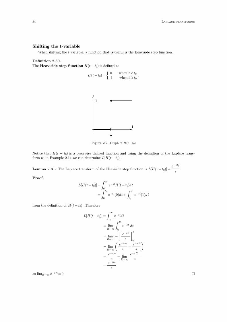
Shifting the t-variable
When shifting the t variable, a function that is useful is the Heaviside step function.
Definition 2.30.
The Heaviside step function H(t− t0) is defined as
H(t− t0)=
{
0 when t< t01 when t> t0
.
0
1
t0
0
1
t0
0
1
t0
1
t 0
1
t0
1
t
Figure 2.2. Graph of H(t− t0)
Notice that H(t − t0) is a piecewise defined function and using the definition of the Laplace trans-form as in Example 2.14 we can determine L[H(t− t0)].
Lemma 2.31. The Laplace transform of the Heaviside step function is L[H(t− t0)] =e−st0
s.
Proof.
L[H(t− t0)] =
∫
0
∞e−stH(t− t0)dt
=
∫
0
t0
e−st(0)dt+
∫
t0
∞e−st(1)dt
from the definition of H(t− t0). Therefore
L[H(t− t0)] =
∫
t0
∞e−stdt
= limR→∞
∫
t0
R
e −st dt
= limR→∞
−[
e−st
s
]
t0
R
= limR→∞
(
e−st0
s− e−sR
s
)
=e−st0
s− lim
R→∞
e−sR
s
=e−st0
s
as limR→∞ e−sR =0. �
84 Laplace transforms

Example 2.32. Sketch the graphs of the following functions
i. y1(t)= sin t when t> 0
ii. y2(t)= sin (t− 2) when t> 2
iii. y3(t)= H(t− 2)sin(t− 2) when t> 0
Answer: The graphs of i) and ii) are
-1
-0.5
0
0.5
1
0 1 2 3 4 5
y1(t)
-1
-0.5
0
0.5
1
0 1 2 3 4 5 6 7 8 9
y2(t)-1
-0.5
0
0.5
1
0 1 2 3 4 5 6 7 8 9
y2(t)-1
-0.5
0
0.5
1
0 1 2 3 4 5 6 7 8 9
y2(t)
The graph of y2(t) is obtained from y1(t) by shifting 2 units to the right. Notice that y2(t) is notdefined for 0 6 t < 2. y3(t) is the product of functions and we use the following table to determine itsgraph
t interval H(t− 2) H(t− 2)sin(t− 2)
06 t < 2 0 0
t> 2 1 sin(t− 2)
so we see that
H(t− 2)sin(t− 2) =
{
0 when 0 6 t < 2sin(t− 2) when t> 2
and therefore the graph of y3(t) is obtained y1(t) by shifting 2 units to the right and taking thegraph to be zero on the interval 0 6 t < 2. Notice that, unlike y2(t), y3(t) is defined for 0 6 t < 2 andthe answer for part iii) is
-1
-0.5
0
0.5
1
0 1 2 3 4 5 6 7 8 9
y3(t)-1
-0.5
0
0.5
1
0 1 2 3 4 5 6 7 8 9
y3(t)-1
-0.5
0
0.5
1
0 1 2 3 4 5 6 7 8 9
y3(t)
We saw in Example 2.32, that H(t − 2)sin(t − 2) is a ‘t-shift’ of sin(t − 2). Below we give a resultthat expresses the Laplace transform of a shifted function H(t − t0)y(t − t0) in terms of the Laplacetransform of the original function
Theorem 2.33. Let L[y(t)] =Y (s). Then
L[H(t− t0)y(t− t0)] = e−st0Y (s).
Proof.
L[H(t− t0)y(t− t0)]=
∫
0
∞e−stH(t− t0)y(t− t0)dt
=
∫
0
t0
e−st(0)y(t− t0)dt+
∫
t0
∞e−st(1)y(t− t0)dt
2.2 Properties of Laplace transforms 85

from the definition of H(t− t0) in Definition 2.30. Therefore
L[H(t− t0)y(t− t0)]=
∫
t0
∞e−sty(t− t0)dt.
Now use the change of variables T = t− t0 in the integral on the right to get
L[H(t− t0)y(t− t0)] =
∫
0
∞e−s(T +t0)y(T )dT
= e−st0
∫
0
∞e−sTy(T )dT
But T is a ‘dummy variable’ in the above integral that is, the integral takes the same value regardlessof the name of the independent variable:
∫
0
∞e−sTy(T )dT =
∫
0
∞e−sty(t)dt.
Therefore
L[H(t− t0)y(t− t0)]= e−st0
∫
0
∞e−sty(t)dt
= e−st0L[y(t)]
= e−st0Y (s)
which is the desired result. �
Using the definition of the inverse Laplace transform and Theorem 2.33 we clearly have
Corollary 2.34. Let L[y(t)]=Y (s). Then
L−1[e−st0Y (s)]= H(t− t0)y(t− t0).
Example 2.35. Sketch the graph of L−1
[
e−3s
s2 +1
]
.
Answer: Notice thate−3s
s2 +1is of the form e−st0Y (s) with e−st0 = e−3s and Y (s)=
1
s2 + 1. Now
Y (s)=1
s2 +1⇒ y(t)= L−1[Y (s)]= sin(t)
and by Corollary 2.34
L−1
[
e−3s
s2 + 1
]
=H(t− 3)y(t− 3)
=H(t− 3)sin(t− 3)
Using the definition of H(t− t0) in Definition 2.30
H(t− 3)sin(t− 3) =
{
0 when 0 6 t < 3sin(t− 3) when t> 3
and following Example 2.32 the graph of H(t− 3)sin(t− 3) is
-1
-0.5
0
0.5
1
0 1 2 3 4 5 6 7 8 9
t
-1
-0.5
0
0.5
1
0 1 2 3 4 5 6 7 8 9
t
86 Laplace transforms

2.2.4 Laplace transform of derivatives
The Laplace transform of the derivative y ′(t) can be expressed in terms of the Laplace transform ofthe original function y(t). This is essentially done by using integration by parts
L[y ′(t)]=
∫
0
∞e−sty ′(t)dt
= limR→∞
∫
0
R
e−sty ′(t)dt
now let
v = e−st du= y ′(t) dt
dv =− se−st dt u = y(t)and so
L[y ′(t)] = limR→∞
∫
0
R
e−sty ′(t)dt
= limR→∞
(
[
e−sty(t)]
0
R+ s
∫
0
R
e−sty(t)dt
)
= limR→∞
(
e−sRy(R) − e0y(0))
+ s limR→∞
∫
0
R
e−sty(t)dt
=
(
limR→∞
e−sRy(R)
)
− y(0)+ sL[y(t)].
(2.43)
and provided limR→∞ e−sRy(R)=0 (as will be the case if y(t) is of exponential order) then we havethat
L[y ′(t)]= sL[y(t)]− y(0) (2.44)
which expresses the Laplace transform of y ′(t) in terms of the Laplace transform of y(t). Note thatthe argument (2.43) is not a proof, we have ignored some continuity issues. The full proof, given inRamkissoon [1], is not required for this course. We give a statement of the hypotheses required for(2.44) in the following theorem.
Theorem 2.36. If y(t) is continuous and of exponential order and y ′(t) is piecewise continuous onevery finite interval then
L[y ′(t)] = sL[y(t)]− y(0).
Proof. Not required. �
By two applications of Theorem 2.36 we can determine the Laplace transform of y ′′(t) in terms ofthe transform of y(t):
L[y ′′(t)] =L
[
(
y ′(t))′]
= sL[y ′(t)]− y ′(0) using (2.44)with y replacedby y ′
= s (sL[y(t)]− y(0))− y ′(0) using (2.44) as it is
which gives us
L[y ′′(t)] = s2L[y(t)]− sy(0)− y ′(0) (2.45)
Similarly, one can apply Theorem 2.36 n times to obtain the Laplace transform of the nth derivative
y(n)(t) in terms of the transform of y(t):
L[y(n)(t)] = snL[y(t)]− sn−1 y(0)− sn−2y ′(0)− sn−3y ′′(0)� − sy(n−2)(0)− y(n−1)(0) (2.46)
The formulae (2.45) and (2.46) require certain continuity conditions to hold. We give a statement ofthese conditions in the following theorem.
2.2 Properties of Laplace transforms 87

Theorem 2.37. If y(t), y ′(t), y ′′(t), � , y(n−1)(t) are continuous and of exponential order and y(n)(t)is piecewise continuous on every finite interval then
L[y(n)(t)] = snL[y(t)]− sn−1 y(0)− sn−2y ′(0)− sn−3y ′′(0)� − sy(n−2)(0)− y(n−1)(0).
Proof. Not required. �
Example 2.38. Use the formula for the Laplace transform of a derivative to determine
i. L[cos(kt)]
ii. L[sinh(kt)]
Answer:
i. Let y(t)= sin(kt).Then y ′(t) = k cos(kt) and applying Theorem 2.36 we have
L[y ′(t)]= sL[y(t)]− y(0)⇒L[k cos(kt)] = sL[sin(kt)]− sin(0)⇒ kL[ cos(kt)] = sL[sin(kt)]− sin(0)
where we used the linearity property of Theorem 2.18 to move the k outside of the Laplacetransform. Then
kL[ cos(kt)]= sk
s2 + k2
as we know L[sin kt] =k
s2 + k2from Example 2.6. Therefore
L[ cos(kt)]=s
s2 + k2
ii. Recall that the hyperbolic cosine cosh(t) and hyperbolic sine sinh(t) are defined as
cosh kt=e kt + e−kt
2
sinh kt=e kt − e−kt
2
(2.47)
and it is easy to check from these definitions that
(cosh kt)′= k sinhkt , (sinh kt)′= k coshkt
cosh(0)= 1 , sinh(0)= 0
Let y(t)= cosh kt. Then y ′(t)= k sinh(kt) and applying Theorem 2.36 we have
L[k sinh(kt)] = sL[cosh kt]− cosh(0)
and as we know L[cosh kt] =s
s2− k2from Example 2.19
kL[sinh(kt)]= s
(
s
s2− k2
)
− 1
⇒ kL[sinh(kt)] =s2− (s2− k2)
s2− k2
and so
L[sinh(kt)] =k
s2− k2.
88 Laplace transforms

2.3 Applications and more properties of Laplace transforms
2.3.1 Solving differential equations using Laplace transforms
We can use the results of the previous sections to solve differential equations, in particular initialvalue problems, that is, differential equations with specified initial values. We illustrate the appli-cation of Laplace transforms to initial value problems in the following examples.
Example 2.39. Solve the differential equation
y ′′− 3y ′ +2y = e3t (2.48)
subject to the initial conditions y(0) = 0, y ′(0) = 0.
Answer: Take the Laplace transform of both sides of the given differential equation
L[y ′′− 3y ′+2y] = L[e3t]
⇒L[y ′′]− 3L[y ′] + 2L[y] =1
s− 3
Using formulae (2.44), (2.45) for the transform of a derivative we have
s2L[y(t)]− sy(0)− y ′(0)− 3(sL[y(t)]− y(0)) +2L[y(t)]=1
s− 3
Substituting the given initial conditions y(0)= 0, y ′(0)= 0 gives
s2L[y(t)]− 3sL[y(t)] + 2L[y(t)]=1
s− 3
For convenience let L[y(t)]=Y (s)
s2Y (s)− 3sY (s) + 2Y (s)=1
s− 3Now solve for Y (s)
(s2− 3s +2)Y (s)=1
s− 3
Y (s)=1
(s2− 3s + 2)(s− 3)
(2.49)
Our required answer is y(t) = L−1[Y (s)]. We use the partial fraction expansion method (as inExample 2.26) to find the inverse transform of (2.49). We first factorize the denominator of Y (s)
1
(s2− 3s +2)(s− 3)=
1
(s− 1)(s− 2)(s− 3)
then by the formula (2.35) the partial fraction expansion is
1
(s− 1)(s− 2)(s− 3)≡ A
s− 1+
B
s− 2+
C
s− 3
where A, B and C need to be determined. Clear denominators
1≡A(s− 2)(s− 3)+ B(s− 1)(s− 3)+C(s− 1)(s− 2) (2.50)
In this case it is easiest to substitute values into (2.50) in order to determine A, B and C. Substi-tuting values s =1, s = 2 and s =3 into (2.50) gives
2.3 Applications and more properties of Laplace transforms 89

s =1
1 =A(− 1)(− 2)+B(0)(− 2)+C(0)(− 1)
⇒ A =1
2
s =2
1 =A(0)(− 1)+ B(1)(− 1)+ C(1)(0)⇒ B =− 1
s = 3
1 =A(1)(0)+B(2)(0)+C(2)(1)
⇒ C =1
2
Therefore
y(t)= L−1[Y (s)]=L−1
[
1
(s2− 3s +2)(s− 3)
]
= L−1
[
1
(s− 1)(s− 2)(s− 3)
]
=L−1
[
1
2
s− 1+
(− 1)
s− 2+
1
2
s− 3
]
=1
2L−1
[
1
s− 1
]
−L−1
[
1
s− 2
]
+1
2L−1
[
1
s− 3
]
=1
2et − e2t +
1
2e3t
and so the solution to this initial value problem is
y(t)=1
2et − e2t +
1
2e3t
It is possible to solve the initial value problem of Example 2.39 by other methods of solving differen-tial equations such as D-operators and power series. One value of using Laplace transforms has overthese other methods is that the inhomogeneous term, usually on the right side of the differentialequation (for example the e3t in equation (2.48)) can be a piecewise defined function as we see in thefollowing example.
Example 2.40. Solve the differential equation
x ′′(t) +x(t) =F (t)
subject to the initial conditions x(0) = 0, x ′(0) = 1 and where F (t) is the piecewise defined function
F (t) =
1 when 06 t <π
2
0 when t>π
2
Answer: Take the Laplace transform of both sides of the given differential equation
L[x′′ +x] =L[F (t)] (2.51)
and so we need to determine L[F (t)]. The graph of F (t) is
90 Laplace transforms

0
1
pi/2
0
1
pi/2
0
1
pi/2
1
t 0
1
pi/2
1
t
One way to determine the Laplace transform of a piecewise defined function is to do so from firstprinciples, that is, using the definition of the Laplace transform as in Example 2.14. Another way isto use Heaviside functions. Consider the following table
t interval H(t− π
2) 1− H(t− π
2) F (t)
0 6 t <π
20 1 1
t >π
21 0 0
and therefore
F (t)= 1− H(t− π
2)
⇒L[F (t)]= L[
1− H(t− π
2)]
=L[1]−L[
H(t− π
2)]
=1
s− e
− sπ
2
s
using Lemma 2.31. Substituting L[F (t)] into (2.51) we have
L[x ′′+x] =1
s− e
− sπ
2
s
⇒ L[x ′′] +L[x] =1
s− e
− sπ
2
s
Using formula (2.45) for the transform of the second derivative we have
s2L[x(t)]− sx(0)− x′(0)+ L[x(t)] =1
s− e
− sπ
2
s
Substituting the given initial conditions x(0) = 0, x′(0)= 1 gives
s2L[x(t)]− 1 +L[x(t)]=1
s− e
− sπ
2
s
For convenience let L[x(t)] =X(s)
s2X(s)− 1 + X(s)=1− e
− sπ
2
sand solve for X(s)
(s2 +1)X(s) =1− e
− sπ
2
s+1
X(s)=1− e
− sπ
2
s(s2 +1)+
1
s2 +1
(2.52)
At this point we use partial fractions to expand
1− e− sπ
2
s(s2 + 1)(2.53)
2.3 Applications and more properties of Laplace transforms 91

In this case it may be best to write (2.53) as
1
s(s2 +1)
(
1− e− sπ
2
)
(2.54)
and apply partial fractions to1
s(s2 + 1):
1
s(s2 + 1)≡ A
s+
Bs+ C
s2 +1
⇒ 1 ≡A(s2 + 1)+ s(Bs +C)
⇒ 1 ≡ (A + B)s2 + Cs + A
and by comparing coefficients of 1, s and s2 we obtain, respectively, three equations
A =1C =0
A +B =0and so
1
s(s2 +1)≡ 1
s− s
s2 +1.
and therefore
1
s(s2 + 1)
(
1− e− sπ
2
)
=
(
1
s− s
s2 + 1
)
(
1− e− sπ
2
)
=1
s− s
s2 +1− e
− sπ
2
s+
se− sπ
2
s2 + 1
and this is the required partial fraction expansion of (2.54). Subtituting this into X(s) in (2.52) wehave
X(s)=1
s+
1
s2 + 1− s
s2 + 1− e
− sπ
2
s+
se− sπ
2
s2 +1and therefore
x(t)=L−1[X(s)]= L−1
1
s+
1
s2 +1− s
s2 +1− e
− sπ
2
s+
s e− sπ
2
s2 + 1
=L−1
[
1
s
]
+L−1
[
1
s2 +1
]
−L−1
[
s
s2 +1
]
−L−1
e− sπ
2
s
+L−1
se− sπ
2
s2 + 1
=1 + sin t− cos t−H(t− π
2)+H(t− π
2)cos(t− π
2)
and so the solution to this initial value problem is
x(t) = 1 + sin t− cos t−H(t− π
2)+H(t− π
2)cos(t− π
2). (2.55)
So when the inhomogeneous part F (t) of our differential equation is piecewise defined, we obtaina solution to the differential equation that is also piecewise defined as we can see by using the defini-tion of the Heaviside function to write (2.55) as
x(t) =
1 + sin t− cos t when 06 t <π
2
1 + sin t− cos t− 1 + cos(t− π
2) when t>
π
2
It is interesting to note that while the inhomogeneous part F (t) of the differential equation ofExample 2.40 is not continuous at t =
π
2(there is a break in the graph of F (t) at t =
π
2), the solution
x(t) given in (2.55) is actually continuous and in fact differentiable at t =π
2as we can see from the
graph of x(t)
92 Laplace transforms

-2
-1
0
1
2
pi/2
x(t)
t
-2
-1
0
1
2
pi/2
x(t)
t
where we have drawn the interval 0 6 t <π
2in solid and the interval t >
π
2in dashes. Notice both
pieces meet smoothly at t =π
2. Also notice from the graph that x(t) satisfies the initial conditions
x(0) = 0, x′(0)= 1.
2.3.2 Solving simultaneous linear differential equations usingthe Laplace transform
We briefly discuss an example that motivates how simultaneous differential equations arise. Thisexample serves only to help illustrate simultaneous differential equations and its details are notrequired for this course.
Example 2.41. Consider a farm with mice and cats. The mouse population changes with time t
and denote this population by M(t). Similarly denote the cat population by C(t). Now the rateM ′(t) at which the mouse population changes at time tdepends on two things
− the number of mice alive at time t (that is M(t)), as more mice present means a greatermouse reproduction rate.
− the number of encounters between cats and mice as the population of mice decreases at theseencounters. For simplicity we assume the number of encounters is proportional to the productM(t)C(t).
Hence M ′(t) is proportional to M(t) and M(t)C(t) and we have the differential equation
M ′(t)= aM(t)− bM(t)C(t)
where a and b are constants such that a, b > 0. Notice that this differs from the differential equationswe have considered so far as there are two dependent variables M, C and one independent variable t.Similarly the rate C ′(t) at which the cat population changes depends on
− the number of encounters between cats and mice as encounters means food for the cats andtherefore an increased survival rate C ′(t) of cats
− the more cats present means less food for each individual cat and therefore an increaseddeath rate C ′(t) of cats
and we have the differential equation
C ′(t)=− dC(t)+ eM(t)C(t)
where d, e > 0. The two equationsM ′(t)= aM(t)− bM(t)C(t)C ′(t)=− dC(t) + eM(t)C(t)
form an example of simultaneous differential equations in which the dependent variables interact2.5.
2.5. This particular system of differential equations is called a Lotka-Volterra system and is used in predator-prey models.
2.3 Applications and more properties of Laplace transforms 93

We now illustrate the solution of simultaneous linear differential equations by using the Laplacetransform.
Example 2.42. Use the Laplace transform to solve the following simultaneous linear differentialequations
y1′ =− y1 + y2
y2′ =− y1− y2
subject to the initial conditions y1(0)= 1 and y2(0)= 0.
Answer: Take the Laplace transform of both equations
L[y1′] =−L[y1] +L[y2]
L[y2′] =−L[y1]−L[y2]
Using formulae (2.44) for the transform of a derivative we have
sL[y1]− y1(0)=−L[y1] +L[y2]sL[y2]− y2(0)=−L[y1]−L[y2]
Substituting the initial conditions y1(0)= 1 and y2(0)= 0 gives
sL[y1]− 1 =−L[y1] +L[y2]sL[y2] =−L[y1]−L[y2]
For convenience let L[y1(t)]= Y1(s) and L[y2(t)] =Y2(s)
sY1(s)− 1 =− Y1(s)+Y2(s)sY2(s)=− Y1(s)− Y2(s)
and we can rewrite these two equations as
− 1 =− (s +1)Y1(s)+Y2(s) (2.56)
0 =−Y1(s)− (s +1)Y2(s) (2.57)
We eliminate Y2(s). Multiplying equation (2.56) by s+ 1 we have
− (s +1) =− (s+ 1)2Y1(s)+ (s + 1)Y2(s) (2.58)
and adding equations (2.57) and (2.58) gives
− (s +1)=− ((s + 1)2 +1)Y1(s)
⇒ Y1(s)=s +1
(s +1)2 + 1From equation (2.57) we know
Y2(s)=− Y1(s)
s +1
⇒ Y2(s)=− 1
(s + 1)2 +1Recall that
L[cos t] =s
s2 +1L[sin t] =
1
s2 + 1
Shifting these along the s-axis gives
L[e−tcos t] =s + 1
(s +1)2 +1L[e−tsin t] =
1
(s +1)2 +1and so
y1(t)= L−1[Y1(s)] y2(t) =L−1[Y2(s)]
=L−1
[
s +1
(s +1)2 +1
]
=L−1
[
− 1
(s +1)2 + 1
]
= e−tcos t =− e−tsin t
94 Laplace transforms
and the solution to our simultaneous linear differential equations is
y1(t) = e−tcos t y2(t)=− e−tsin t.
2.3.3 Convolution and Integral equations
Recall from Lemma 2.22 that the inverse Laplace transform of a sum is the sum of inverse trans-forms
L−1[Y1(s) +Y2(s)]= L−1[Y1(s)] +L−1[Y2(s)].
However, a similar statement does NOT hold for products. In general
L−1[Y1(s)Y2(s)] � L−1[Y1(s)]L−1[Y2(s)] (2.59)
as the following example demonstrates: consider Y1(s)=1
sand Y2(s)=
1
s. Then
L−1[Y1(s)Y2(s)] =L−1
(
1
s
1
s
)
L−1[Y1(s)]L−1[Y2(s)]=L−1
(
1
s
)
L−1
(
1
s
)
=L−1
[
1
s2
]
=1 . 1
= t = 1
and clearly this is a case of (2.59).
In order to obtain a formula for L−1[Y1(s)Y2(s)] where Y1(s) and Y2(s) are Laplace transforms, weshall need the following
Definition 2.43. The convolution of f(t) and g(t) is denoted as f ∗ g and is defined as
(f ∗ g)(t) =
∫
0
t
f(t− β)g(β)dβ.
Example 2.44. Find the convolution f ∗ g when f(t) = t2 and g(t) = t, that is, find t2 ∗ t.
Answer: Replacing the variable t with t− β in f(t) = t2 gives
f(t− β)= (t− β)2
and similarly we obtain g(β) = β. Then
(f ∗ g)(t) = t2 ∗ t
=
∫
0
t
(t− β)2β dβ
=
∫
0
t
(t2− 2tβ + β2)β dβ
=
∫
0
t
(t2β − 2tβ2 + β3) dβ
=
[
t2β2
2− 2tβ3
3+
β4
4
]
0
t
=t4
2− 2t4
3+
t4
4
=t4
12and so
t2 ∗ t=t4
12.
Notice from Definition 2.43 and Example 2.44 that if f , g are functions of t then f ∗ g is again afunction of t. We now give a formula for L−1[Y1(s)Y2(s)] in the theorem below.
2.3 Applications and more properties of Laplace transforms 95

Theorem 2.45. (Convolution Theorem) If Y1(s)=L[y1(t)] and Y2(s) =L[y2(t)] then
L−1[Y1(s)Y2(s)]= y1 ∗ y2
or equivalently
L[y1 ∗ y2] =L[y1(t)]L [y2(t)].
Proof. Not required. �
Example 2.46. Find L−1
[
2
s5
]
by using the Convolution Theorem.
Answer: We can split2
s5as a product in several ways. Let us choose one such way
Y1(s)=2
s3Y2(s)=
1
s2.
and using the formula L[tn] =n!
sn+1
y1(t)=L−1[Y1(s)]= t2 y2(t)=L−1[Y2(s)]= t
Then using the Convolution Theorem
L−1
[
2
s5
]
=L−1
[
2
s3
1
s2
]
= L−1[Y1(s)Y2(s)]= y1 ∗ y2
= t2 ∗ tand from Example 2.44
t2 ∗ t =t4
12therefore
L−1
[
2
s5
]
=t4
12.
Of course, we did not need to use the Convolution Theorem to determine L−1
[
2
s5
]
, we can use the
formula L[tn] =n!
sn+1 directly. On the other hand, examples in which the Convolution Theorem is
needed are given by integral equations.
Definition 2.47. An equation which contains the dependent unknown variable under an integraloperator is called an integral equation.
We will be interested in those integral equations that can be solved by using Laplace tranforms andthe Convolution theorem.
Example 2.48. Use the Laplace transform to solve the integral equation
y(t)= 4t− 3
∫
0
t
sin(t− β)y(β)dβ.
Answer: Take the Laplace transform of both sides of the integral equation
L[y(t)] =L[4t]− 3L
[ ∫
0
t
sin(t− β)y(β)dβ
]
.
Notice that the integral∫
0
t
sin(t− β)y(β)dβ (2.60)
96 Laplace transforms

is in the form of a convolution, that is∫
0
t
sin(t− β)y(β)dβ = sin t ∗ y(t)
and from the Convolution Theorem
L
[ ∫
0
t
sin(t− β)y(β)dβ
]
= L[sin t ∗ y(t)] =L[sin t]L[y(t)]. (2.61)
Substituting (2.61) into (2.60) we have
L[y(t)]=L[4t]− 3L[sin t]L[y(t)]
and denoting L[y(t)] =Y (s)
Y (s) =4
s2− 3
(
1
s2 +1
)
Y (s)
⇒ Y (s)
(
1− 3
s2 +1
)
=4
s2
⇒ Y (s)
(
s2 +4
s2 +1
)
=4
s2
⇒ Y (s)=4(s2 + 1)
s2(s2 +4)and using partial fractions
4(s2 +1)
s2(s2 +4)≡ A
s+
B
s2+
Cs +D
s2 + 4
⇒ 4s2 +4≡As(s2 +4)+ B(s2 + 4)+ (Cs +D)s2
⇒ 4s2 +4≡ (A +C)s3 + (B +D)s2 + 4As +4B
and by comparing coefficients of 1, s , s2 and s3 we obtain, respectively, four equations
4B =44A = 0
B + D = 4A +C = 0
Solving these gives A =0, B =1, C =0,D =3 and therefore
Y (s) =1
s2+
3
s2 + 4
and so the answer to our integral equation is y(t) where
y(t)= L−1[Y (s)]= L−1
[
1
s2
]
+ L−1
[
3
s2 + 4
]
= L−1
[
1
s2
]
+3
2L−1
[
2
s2 +22
]
= t+3
2sin(2t).
2.3.4 Dirac’s delta function
Dirac’s delta function δ(t) is not actually a function of the variable t. It is a distribution. Thetheory of distributions belongs to a branch of mathematics called functional analysis. We shall dis-cuss the proof of the formula
L[δ(t)] = 1 (2.62)
which can more generally be stated as
L[δ(t− t0)]= e−st0 where t0 > 0 (2.63)
2.3 Applications and more properties of Laplace transforms 97

however this proof is not required for this course. Knowledge and application2.6of the two formulae(2.62) and (2.63) is the only requirement of this subsection.
In functional analysis, a functional is a map from a set of functions to a set of numbers.
Example 2.49. Let C denote the set of continuous functions and R denote the set of real numbers.Then
i. the map φ: C→R defined by
φ(f) =
∫
a
b
f(t)dt
is a functional as integrating any continuous function f(t) over a finite interval [a, b] gives anumber.
ii. the map σ: C→R defined by
σ(f)= f(0)
is also a functional. Notice that σ associates to any continuous function f(x) the value ofthat function at t=0.
One can define functionals on many sets of functions, in the Example 2.49 above we described twodifferent functionals on a particular set of functions – the set of continuous functions C. To definethe Dirac delta function we shall need another specific set of functions – the set of test functions.Denote the set of test functions as D.
Definition 2.50. A test function on R is a function that is identically zero outside a sufficientlylarge interval − c < t < c and that has derivatives of any order.
Recall that as any differentiable function is necessarily continuous, it follows that D ⊂ C, that is theset of test functions on R is contained in the set of continuous functions on R.
Example 2.51. The function
f(t)=
e− 1
1−t2 when − 1 <t < 10 when t6− 1 or t> 1
is an example of a test function. From the graph of f(t)
0-1 0 1
f(t)
0-1 0 1
f(t)
0-1 0 1
f(t)
it is clear that f(t) is identically zero outside − 1<t < 1. Notice that f(t) is a continuous function.
Definition 2.52. Let D denote the set of all test functions on R. Then a functional that hasdomain equal to D is called a distribution on R.
We can now give a precise definiton of the Dirac delta function δ(t).
2.6. see Example 2.63
98 Laplace transforms

Definition 2.53.The Dirac delta function δ(t) is the distribution δ(t): D→R that is defined as
δ(t)(φ)= φ(0).
So the Dirac delta function δ(t) maps any test function φ in the set D to a corresponding numberφ(0). In other words, δ(t) takes any test function φ and evaluates that function at t = 0. More gener-ally, we can define the ‘shifted’ Dirac delta function δ(t− t0).
Definition 2.54.The Dirac delta function δ(t− t0) is the distribution δ(t− t0): D→R that is defined as
δ(t− t0)(φ)= φ(t0)
where t0 > 0 is a constant.
Notice by letting t0 =0, Definition 2.54 reduces to Definition 2.53.
We now give a more intuitive but less technically accurate description of the Dirac delta functionδ(t− t0). Consider the following function
fn(t)=
n when t0 6 t6 t0 +1
n0 otherwise
(2.64)
where n= 1, 2, 3,� is a parameter that can vary. The graph of fn(t) is
n
t0+1/nt0
fn(t)
t
n
t0+1/nt0
fn(t)
t
and we see that the graph of fn(t) takes the form of a pulse. Notice that the area under this graph isn(t0 +
1
n− t0) = 1. Now as the parameter n gets larger, the ‘pulse’ fn(t) gets narrower and higher.
We see this in the graphs below illustrating the cases n = 1, 2, 3 respectively:
1
t0+1
f1(t)
t
1
t0+1
f1(t)
t
2
t0+1/2
f2(t)
t
2
t0+1/2
f2(t)
t
3
t0+1/3
f3(t)
t
3
t0+1/3
f3(t)
t
Notice that the area under the graph of each f1, f2 and f3 is 1.
Intuitively, as n→∞ the functions fn tend to the Dirac delta function, that if it were to exist asa function, would take the form of a pulse with zero width, infinite height and an area of 1.
2.3 Applications and more properties of Laplace transforms 99

The above intuitive description of the Dirac delta function is not precise as the pointwise limit ofthe functions fn(t) as n→∞
limn→∞
fn(t)
does not exist. If the limit limn→∞ fn(t) were to exist then for any value t = a, the sequence of num-bers fn(a) would converge. However, when t = t0 the sequence of numbers f1(t0), f2(t0), f3(t0), � isequal to 1, 2, 3, � which is a sequence that does not converge. Therefore the pointwise limitlimn→∞ fn(t) does not exist.
However, it turns out that the theory of distributions was developed to handle such situations astaking the limit of the sequence fn above. In the theory of distributions, each function fn can beconverted into a corresponding distribution which is denoted by Tfn
. Then one takes the limit of
these distributions – this is actually a limit of integrals. In this particular case, the limit of the Tfn
as n→∞ does exist and is in fact equal to the distribution δ(t− t0) as defined in Definition 2.54. Itis in this sense of distributions that the above sequence fn converge to the Dirac delta δ(t− t0).
The following definition describes how a function fn is converted to a distribution Tfn.
Definition 2.55. Let f(t) be a function that is locally integrable, that is,∫
a
bf(t)dt < ∞ for any
finite interval a < x < b. Then the distribution Tf:D→R associated to the function f(t) is defined as
Tf(φ) =
∫
−∞
∞fφ dt
where φ is any test function in D.
Example 2.56. Let fn be the function defined in (2.64). Then
Tfn(φ) =
∫
−∞
∞fnφ dt
=n
∫
t0
t0+1
n
φdt.
Let Tn n = 1, 2, 3,� be a sequence of distributions. Then notice for a fixed test function φ, Tn(φ) isa sequence of real numbers. We now describe the limit of a sequence of distributions.
Definition 2.57. The sequence of distributions Tn n = 1, 2, 3, � has limit equal to the distributionT0 only if for each test function φ the sequence of real numbers Tn(φ) has limit equal to T0(φ).
In other words Tn → T0 as distributions only if Tn(φ) → T0(φ) as real numbers for each test functionφ. The following lemma will be useful in proving that the ‘pulse’ functions fn defined in (2.64) haslimit equal to the Dirac delta function δ(t − t0) in the sense of distributions, that is, Tfn
→ δ(t − t0)as n→∞.
Lemma 2.58. Let φ(t) be a continuous function and let fn be defined as in equation (2.64) above.Then
limn→∞
∫
−∞
∞fn(t)φ(t)dt= φ(t0).
Proof. From equation (2.64)
∫
−∞
∞fn(t)φ(t)dt= n
∫
t0
t0+1
n
φ(t)dt.
=n
∫
t0
t0+1
n
(φ(t)− φ(t0)+ φ(t0) )dt
=n
∫
t0
t0+1
n
(φ(t)− φ(t0))dt+n
∫
t0
t0+1
n
φ(t0)dt
(2.65)
100 Laplace transforms

Let us consider the first integral on the right. As φ(t) is continuous at t = t0, by the definition ofcontinuity, given any ǫ > 0 there exists a δ > 0 such that
− ǫ < (φ(t)− φ(t0)) <ǫ when − δ < t− t0 <δ. (2.66)
Now as δ > 0, there exists an integer N such that1
n< δ for all n > N . Integrating the first inequality
in (2.66) between t0 +1
nand t0 for any n > N gives
∫
t0
t0+1
n
(− ǫ)dt <
∫
t0
t0+1
n
(φ(t)− φ(t0))dt <
∫
t0
t0+1
n
ǫdt (2.67)
and as ǫ is independent of t, it is easy to evaluate the first and third inequalities in (2.67)
− ǫ
n<
∫
t0
t0+1
n
(φ(t)− φ(t0))dt<ǫ
n
and multiplying throughout by n we have
− ǫ <n
∫
t0
t0+1
n
(φ(t)− φ(t0))dt < ǫ. (2.68)
We have shown that for any ǫ > 0 there exists some N such that for all n > N the inequality (2.68)holds. As this is true for any ǫ > 0, we can make ǫ in (2.68) as small as we wish, this thereforeimplies that
limn→∞
n
∫
t0
t0+1
n
(φ(t)− φ(t0))dt
=0. (2.69)
Now consider the second integral on the right in the last line of (2.65). As φ(t0) is a constant
n
∫
t0
t0+1
n
φ(t0)dt=nφ(t0) [t]t0t0+
1
n = φ(t0)
and therefore∫
−∞
∞fn(t)φ(t)dt = n
∫
t0
t0+1
n
(φ(t)− φ(t0))dt+n
∫
t0
t0+1
n
φ(t0)dt
⇒∫
−∞
∞fn(t)φ(t)dt =
n
∫
t0
t0+1
n
(φ(t)− φ(t0))dt
+ φ(t0)
Taking the limit as n→∞ gives
limn→∞
∫
−∞
∞fn(t)φ(t)dt = lim
n→∞
n
∫
t0
t0+1
n
(φ(t)− φ(t0))dt
+ limn→∞
φ(t0)
From (2.69) we have
limn→∞
∫
−∞
∞fn(t)φ(t)dt = 0 + lim
n→∞φ(t0)
and as φ(t0) is a constant we get our desired result
limn→∞
∫
−∞
∞fn(t)φ(t)dt = φ(t0). �
We now use Lemma 2.58 to show that the ‘pulse’ functions fn defined in (2.64) has limit equal tothe Dirac delta function δ(t− t0) in the sense of distributions.
Lemma 2.59. Let fn be defined as in equation (2.64) and let Tfnbe the corresponding distribu-
tions as in Definition 2.55. Then as n→∞Tfn
→ δ(t− t0)
2.3 Applications and more properties of Laplace transforms 101

as distributions.
Proof. By Definition 2.57 Tfn→ δ(t− t0) as n→∞ if for each test function φ,
limn→∞
Tfn(φ)= δ(t− t0)(φ) (2.70)
Now from Definition 2.55
Tfn(φ) =
∫
−∞
∞fnφ dt
and from the definition of the Dirac delta as a distribution in Definition 2.54
δ(t− t0)(φ)= φ(t0).
Substituting these two definition into (2.70) we have that Tfn→ δ(t − t0) as n → ∞ if for each test
function φ
limn→∞
∫
−∞
∞fnφdt = φ(t0). (2.71)
However since any test function φ is continuous, (2.71) is true from Lemma 2.58 and therefore theresult follows.
�
We now determine the Laplace transform of the Dirac delta function δ(t− t0). Recall that δ(t− t0) isa distribution. The following is the definition of the Laplace transform of a distribution (also seeReinhard [3]).
Definition 2.60.
Let
φs =
{
0 when t< 0
e−st when t> 0
If T is a distribution and if T (φs) exists then T has Laplace transform
L[T ] =T (φs)
where T (φs) is the evaluation of the functional T at the function φs.
Using this definition we have
Theorem 2.61. The Laplace transform of the Dirac delta function δ(t− t0) where t 0 > 0 is
L[δ(t− t0)]= e−st0. (2.72)
Proof. As stated in Definition 2.54 the Dirac delta is a distribution. As a functional δ(t − t0) takesany function φ and evaluates that function at t = t0, hence the functional δ(t − t0) takes the functionφs and evaluates it at t= t0, that is
δ(t− t0)(φs)= e−st0
as t0 > 0. By Definition 2.60 we have
L[δ(t− t0)]= δ(t− t0)(φs)= e−st0.
�
By letting t0 =0 in the formula (2.72) we have the following
Corollary 2.62. The Laplace transform of the Dirac delta function δ(t) is
L[δ(t)]= 1.
102 Laplace transforms

In this course we shall treat δ(t − t0) as a function. The above precisedefinition of δ(t − t0) is only for the interest of the reader, it is notrequired material. Knowledge of the formulae
L[δ(t− t0)]= e−st0
L[δ(t)] = 1
is required as is the application of these formulae as done in the fol-lowing example.
Example 2.63. Solve the differential equation
y ′′+ 9y = δ(t− 1) (2.73)
subject to the initial conditions y(0) = 0, y ′(0) = 0.
Answer: Take the Laplace transform of both sides of the given differential equation
L[y ′′+9y] =L[δ(t− 1)]
⇒ L[y ′′] + 9L[y] = e−s
Using formula (2.45) for the transform of the second derivative we have
s2L[y(t)]− sy(0)− y ′(0)+ 9L[y(t)] = e−s
Substituting the given initial conditions y(0)= 0, y ′(0)= 0 gives
s2L[y(t)]+ 9L[y(t)]= e−s
Let L[y(t)] =Y (s)
s2Y (s)+ 9Y (s)= e−s
Now solve for Y (s)
(s2 +9)Y (s) = e−s
Y (s)=e−s
(s2 +9)= e−s1
3
3
(s2 +32)
Notice that e−s 1
3
3
(s2 +32)is of the form e−st0Y (s) with e−st0 = e−s and Y (s) =
1
3
3
(s2 + 32). Now
Y (s)=1
3
3
(s2 +32)⇒ y(t)=L−1[Y (s)] =
1
3sin(3t)
and by the ‘t-shift’ formula of Corollary 2.34
L−1
[
e−s1
3
3
(s2 + 32)
]
=H(t− 1)y(t− 1)
=H(t− 1)1
3sin(3(t− 1))
and so the solution to this initial value problem is
y(t)= H(t− 1)1
3sin(3(t− 1)).
One can associate a physical interpretation to Example 2.63. The homogeneous part of the differ-rential equation (2.73), that is
y ′′ +9y =0
is an equation that describes some type of oscillation about an equilibrium position, for example thesimple harmonic motion of a mass loaded on a spring, where y measures the displacement from theequilibrium position
2.3 Applications and more properties of Laplace transforms 103

y = 0(equilibrium position)y
The inhomegeneous part of the differential equation
y ′′+ 9y = δ(t− 1) (2.74)
that is, the right hand side of the equation (2.74), may be interpreted in our example of a spring asa vertical outside force applied to the mass over time. In this case δ(t − 1) can be viewed as asudden impulse at an instant of time when t=1.
Now the initial condition y(0) = 0 means that the mass is at the equilibrium position at time t =0. The condition y ′(0) = 0 means that the velocity at time t = 0 is zero. The mass is therefore at restand does NOT move until time t = 1 when the impulse δ(t − 1) is applied, causing the mass to oscil-late as we can see from the following graph of the solution
y(t)= H(t− 1)1
3sin(3(t− 1)) (2.75)
of the differential equation (2.74)
1/3
1
y(t)
t
1/3
1
y(t)
t
Also notice from the graph of y(t) that after time t = 1 the system oscillates freely about the equilib-rium position as there is no outside force after t= 1.
104 Laplace transforms

2.3.5 Differentiation of transforms
The result given in the following is useful for determining tranforms and inverse transforms.
Theorem 2.64. If Y (s) = L[y(t)] then Y ′(s) = L[ − ty(t)] where Y ′(s) denotes the derivative ofY (s) with respect to the variable s.
Proof. From the definition of the Laplace transform
Y (s)=
∫
0
∞e−sty(t)dt
and differentiating both sides of this equation with respect to s gives
Y ′(s) =d
ds
∫
0
∞e−sty(t)dt. (2.76)
It is possible to 2.7exchange the differentiation and integration operations in equation (2.76)
Y ′(s) =
∫
0
∞ d
ds(e−sty(t))dt
and differentiating e−sty(t) partially with respect to s we have
Y ′(s) =
∫
0
∞− te−sty(t) dt
=
∫
0
∞e−st(− ty(t)) dt
= L[− ty(t)].
�
The following two examples are applications of Theorem 2.64.
Example 2.66. Find L[t sin t].
Answer:
L[sin t] =1
s2 +1and by Theorem 2.64
L[− t sin t] =
(
1
s2 +1
)′
=− 2s
(s2 + 1)2
and therefore by linearity
L[t sin t] =2s
(s2 + 1)2.
Using Theorem 2.64 gives a more efficient method of proving L[tn] =n!
sn+1 than Example 2.7.
Example 2.67. Use the principle of induction, the definition of the Laplace transform and Theorem2.64 to show that
L[tn] =n!
sn+1
when n = 0, 1, 2,�2.7. This is done by an application of the following
Lemma 2.65. Let y(s, t) and∂y(s, t)
∂sbe continuous on the set {(s, t)|c6 s6 d, 0 6 t <∞}; let the integral
∫
0
∞ ∂y(s, t)
∂sdt
be uniformly convergent and denote Y (s)=∫
0
∞
y(s, t) dt. Then Y (s) is differentiable and
Y ′(s)=
∫
0
∞ ∂y(s, t)
∂sdt.
Knowledge of this lemma is not required for this course.
2.3 Applications and more properties of Laplace transforms 105

Answer: The statement is true when n = 0 as
L[t0] =L[1]
=
∫
0
∞e−stdt
= limR→∞
∫
0
R
e−stdt
= limR→∞
[
e−st
− s
]
0
R
= limR→∞
(
1
s− e−sR
s
)
=1
swhen s > 0
=0!
s0+1
Assume the statement is true when n = k, that is
L[tk] =k!
sk+1.
Then by using Theorem 2.64
L[− t.tk] =
(
k!
sk+1
)′
⇒L[− tk+1] = k!
(
1
sk+1
)′
= k!
(
− (k +1)
sk+2
)
=− (k +1)!
sk+2
and therefore
L[tk+1] =(k +1)!
sk+2
and so the statement is true when n= k + 1, hence by the principle of induction
L[tn] =n!
sn+1
is true for all n =0, 1, 2,�2.3.6 The Gamma function Γ(x)
In Examples 2.7 and 2.67 we obtained the formula
L[tn] =n!
sn+1
when n = 0, 1, 2, � . We now wish to obtain a more general formula, that is, a formula for L[tx]when x is a real number and x >− 1. To do this, we need to define the gamma function Γ(x).
Definition 2.68. The gamma function Γ(x) is defined when x > 0 as an integral
Γ(x) =
∫
0
∞e−ttx−1 dt. (2.77)
The following result gives some properties of the gamma function.
Lemma 2.69. Let Γ(x) denote the gamma function. Then
i. Γ(1)= 1
ii. Γ(x +1)= xΓ(x) when x > 0
iii. Γ(n +1)= n! when n =0, 1, 2,�
106 Laplace transforms
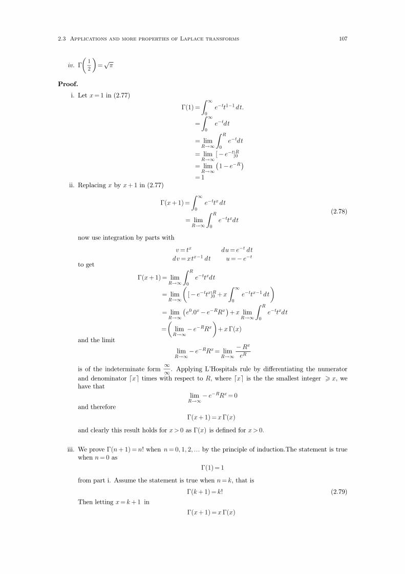
iv. Γ
(
1
2
)
= π√
Proof.
i. Let x =1 in (2.77)
Γ(1) =
∫
0
∞e−tt1−1 dt.
=
∫
0
∞e−tdt
= limR→∞
∫
0
R
e−tdt
= limR→∞
[− e−t]0R
= limR→∞
(
1− e−R)
=1ii. Replacing x by x+ 1 in (2.77)
Γ(x +1)=
∫
0
∞e−ttx dt
= limR→∞
∫
0
R
e−ttxdt
(2.78)
now use integration by parts with
v = tx du = e−t dt
dv =xtx−1 dt u =− e−t
to get
Γ(x +1)= limR→∞
∫
0
R
e−ttxdt
= limR→∞
(
[− e−ttx]0R +x
∫
0
∞e−ttx−1 dt
)
= limR→∞
(
e0.0x− e−RRx)
+x limR→∞
∫
0
R
e−ttxdt
=
(
limR→∞
− e−RRx
)
+ xΓ(x)
and the limit
limR→∞
− e−RRx = limR→∞
−Rx
eR
is of the indeterminate form∞∞ . Applying L’Hospitals rule by differentiating the numerator
and denominator ⌈x⌉ times with respect to R, where ⌈x⌉ is the the smallest integer > x, wehave that
limR→∞
− e−RRx =0
and therefore
Γ(x+1) =x Γ(x)
and clearly this result holds for x > 0 as Γ(x) is defined for x > 0.
iii. We prove Γ(n + 1) = n! when n = 0, 1, 2,� by the principle of induction.The statement is truewhen n = 0 as
Γ(1)= 1
from part i. Assume the statement is true when n = k, that is
Γ(k + 1)= k! (2.79)
Then letting x = k + 1 in
Γ(x+1) =x Γ(x)
2.3 Applications and more properties of Laplace transforms 107
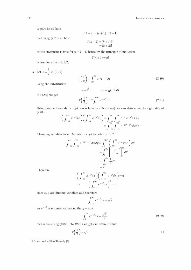
of part ii) we have
Γ(k +2) = (k + 1)Γ(k + 1)
and using (2.79) we haveΓ(k +2)= (k +1)k!
= (k + 2)!
so the statement is true for n = k +1, hence by the principle of induction
Γ(n +1)= n!
is true for all n =0, 1, 2,�iv. Let x =
1
2in (2.77)
Γ
(
1
2
)
=
∫
0
∞e−tt
− 1
2 dt (2.80)
using the substitution
u = t1
2 du =1
2t− 1
2 dt
in (2.80) we get
Γ
(
1
2
)
=2
∫
0
∞e−u2
du (2.81)
Using double integrals (a topic done later in this course) we can determine the right side of(2.81)
( ∫
−∞
∞e−x2
dx
)( ∫
−∞
∞e−y2
dy
)
=
∫
−∞
∞ ∫
−∞
∞e−x2
e−y2
dxdy
=
∫
−∞
∞ ∫
−∞
∞e−(x2+y2)dxdy
Changing variables from Cartesian (x, y) to polar (r, θ)2.8
∫
−∞
∞ ∫
−∞
∞e−(x2+y2)dxdy =
∫
0
2π( ∫
0
∞e−r2
rdr
)
dθ
=
∫
0
2π[
− e−r2
2
]
0
∞
dθ
=
∫
0
2π 1
2dθ
=πTherefore
( ∫
−∞
∞e−x2
dx
)( ∫
−∞
∞e−y2
dy
)
= π
⇒( ∫
−∞
∞e−x2
dx
)2
=π
since x, y are dummy variables and therefore∫
−∞
∞e−x2
dx= π√
As e−x2
is symmetrical about the y − axis∫
0
∞e−x2
dx =π
√
2(2.82)
and substituting (2.82) into (2.81) we get our desired result
Γ
(
1
2
)
= π√
. �
2.8. see Section 9.3 of Kreyszig [2]
108 Laplace transforms

Having defined the gamma function, we can now determine L[tx] when x >− 1.
Theorem 2.70.Let x be a real number such that x >− 1. Then
L[tx] =Γ(x +1)
sx+1.2.9
Proof. Substitute x+ 1 for x in the definition of Γ(x)
Γ(x+ 1)=
∫
0
∞e−ttx dt
Using the substitution
t= su dt= sdu
where we treat s as a constant and u as the variable, we get
Γ(x+ 1)=
∫
0
∞e−su(su)x s du
= sx+1
∫
0
∞e−suux du
and as u is a dummy variable, we can replace u by another dummy variable t to get
Γ(x+ 1)= sx+1
∫
0
∞e−sttx dt 2.10
and from the definition of the Laplace transform of tx
Γ(x +1)= sx+1L[tx]
which gives our desired result
L[tx] =Γ(x +1)
sx+1. (2.83)
�
The following is an application of Theorem 2.70.
Example 2.71. Show that L
[
t5
2
]
=15 π√
8s7
2
.
By Theorem 2.70
L
[
t5
2
]
=Γ(
7
2
)
s7
2
and from Lemma 2.69 part ii)
Γ
(
7
2
)
=5
2Γ
(
5
2
)
and applying Lemma 2.69 part ii) two more times we have
Γ
(
7
2
)
=5
2Γ
(
5
2
)
=5
2
(
3
2Γ
(
3
2
))
=5
2
3
2
1
2Γ
(
1
2
)
2.9.Werequirex>− 1 because in the definition of Γ(x) wehavex > 0
2.10. If s < 0 then the integral diverges from Lemma 2.3. and clearly (2.83) is undefined for s = 0, so it is necessary that s >
0 for (2.83) to hold.
2.3 Applications and more properties of Laplace transforms 109

and from Lemma 2.69 part iv)
Γ
(
7
2
)
=5
2
3
2
1
2π
√=
15 π√
8and therefore
L
[
t5
2
]
=15 π√
8s7
2
.
110 Laplace transforms

Chapter 3
Fourier series
3.1 Definitions
Definition 3.1. Let f (x) be a function that is defined for all x. Then f(x) is called periodic ifthere exists a positive number p such that
f(x+ p)= f(x)
for each x. The number p is called a period of the function f(x).
Example 3.2. The function sinx has period p =2π as one can check
sin(x+ 2π)= sin(x) (3.1)
by using the trigonometric formula sin(x + y)= sinx cos y + cosx sin y:
sin(x +2π) = sin(x)cos(2π)+ cos(x)sin(2π)= sin(x).(1)+ cos(x).(0)= sin(x)
Equation (3.1) can be interpreted graphically as follows. The graph of sin(x + 2π) is a shift of thegraph of sin(x) to the left by 2π units. Notice that this ‘shifted’ graph sin(x + 2π) coincides with theoriginal sin(x) and this implies equality in (3.1).
-1
0
1
sin(x)
period= 2pi
Note 3.3. In the following, we shall always let the period p = 2L. We do this to be consistent withnotation used in a later section of partial differential equations. For example, in the case of Example3.2, sin(x) has period 2L= 2π and clearly L =π.
Definition 3.4. Let the functionf(x) be a periodic function of period 2L. Then
a0
2+∑
n=1
∞(
ancosnπx
L+ bnsin
nπx
L
)
(3.2)
111

is a Fourier series for f(x) if its coefficients are given by the formulae
an =1
L
∫
−L
L
f(x)cosnπx
Ldx where n =0, 1, 2, 3,� (3.3)
bn =1
L
∫
−L
L
f(x)sinnπx
Ldx where n =1, 2, 3,� (3.4)
Equations (3.3) and (3.4) are called Euler’s formulae and the numbers an, bn are called theFourier coefficients of f(x).
Example 3.5. Let
f(x) =x where − π <x 6π and f(x +2π) = f(x) (3.5)
Sketch the graph of f(x) and find the Fourier series of f(x) on the interval (−π, π).
Answer: Note that the function f(x) is defined to be periodic with period 2π by the statement
f(x+ 2π)= f(x)
in (3.5). The graph of f(x) is obtained by first drawing f(x) = x on the interval − π < x 6 π andthen repeatedly shifting this drawing by multiples of 2π
Figure 3.1. Graph of f (x)
Notice the closed dots of Figure 3.1 imply that f(x)=π when x =� ,− π, π, 3π, 5π,�We need to determine the Fourier coefficients an and bn. It is typical to split the case of an into
two subcases n =0 and n = 1, 2,� this is because n = 0 causes the cosine term in (3.3) to become 1.
a0 =1
L
∫
−L
L
x cos0πx
Ldx
=1
π
∫
−π
π
x cos 0dx as L= π
=1
π
∫
−π
π
xdx as cos 0 =1
=1
π
[
x2
2
]
−π
π
=0
112 Fourier series

and so
a0 = 0 (3.6)
Now determine anwhen n= 1, 2,�an =
1
L
∫
−L
L
x cosnπx
Ldx
=1
π
∫
−π
π
x cosnπx
πdx
=1
π
∫
−π
π
x cosnx dx notice the π ′s cancel.
Integrating by parts with
v =x du = cosnxdx
dv =1 dx u =sinnx
ngives
an =1
π
[
x sinnx
n
]
−π
π
− 1
π
∫
−π
π sinnx
ndx
=1
π
[
x sinnx
n
]
−π
π
+1
π
[ cosnx
n2
]
−π
π
=1
π
((
π sinnπ
n+
cosnπ
n2
)
−(
− π sin (−nπ)
n+
cos (−nπ)
n2
))
recall when n is an integer
expression value
sinnπ 0
sin (−nπ) 0
cosnπ (− 1)n
cos (−nπ) (− 1)n
Table 3.1.
and therefore
an =1
π
((
0 +(− 1)n
n2
)
−(
0 +(− 1)n
n2
))
which gives
an =0 when n = 1, 2, 3,� (3.7)
And now determine the bn when n =1, 2,�bn =
1
L
∫
−L
L
x sinnπx
Ldx
=1
π
∫
−π
π
x sinnπx
πdx
=1
π
∫
−π
π
x sinnx dx
Integrating by parts with
v =x du = sinnxdx
dv = 1 dx u =− cosnx
n
3.1 Definitions 113
gives
bn =1
π
[
− x cosnx
n
]
−π
π− 1
π
∫
−π
π
− cosnx
ndx
=1
π
[
− x cosnx
n
]
−π
π+
1
π
[
sinnx
n2
]
−π
π
=1
π
((
− π cosnπ
n+
sinnπ
n2
)
−(
− − π cos (−nπ)
n+
sin (−nπ)
n2
))
and using the values from Table 3.1
bn =1
π
((
− π(− 1)n
n+0
)
−(
− − π (− 1)n
n+0
))
=1
π
(
− π(− 1)n
n− π (− 1)n
n
)
=− 2(− 1)n
nwhich gives
bn =2(− 1)n+1
nwhen n =1, 2, 3,� (3.8)
Substituting L =π and the expressions for a0, an and bn given by (3.6),(3.7) and (3.8) into
a0
2+∑
n=1
∞(
ancosnπx
L+ bnsin
nπx
L
)
we get our answer
the Fourier series of the function f(x) given in (3.5) is
∑
n=1
∞2(− 1)n+1
nsinnx.
3.2 Convergence of Fourier Series
In Example 3.5 we proved that the Fourier series of
f(x)=x where −π < x6 π and f(x+ 2π)= f(x) (3.9)
is
∑
n=1
∞2(− 1)n+1
nsinnx. (3.10)
We will see, from Theorem 3.8 and Example 3.9 below that the function f(x) given in (3.9) con-verges to its Fourier series (3.10) for all values of x except when x =� ,− π, π, 3π, 5π,�Definition 3.6.
Suppose
a0
2+∑
n=1
∞(
ancosnπx
L+ bnsin
nπx
L
)
(3.11)
114 Fourier series

is the Fourier series of a function g(x). Let
a0
2+∑
n=1
m(
ancosnπx
L+ bnsin
nπx
L
)
(3.12)
be the sum of the first m terms of (3.11). Then the Fourier series (3.11) is said to converge to g(x)at x= x0 if
limm→∞
(
a0
2+∑
n=1
m(
ancosnπx0
L+ bnsin
nπx0
L
)
)
= g(x0).
Intuitively Definition 3.6 means that the sum of the first m terms (3.12) of the Fouries series isan ‘approximation’ of the function g(x), and this approximation gets better as m gets larger. Let usreturn to our example of f(x) given in (3.9), in which the Fourier series (3.10) converges to f(x)except when x=� ,− π, π, 3π, 5π,�Consider when m = 5, that is the sum of the first five terms of (3.10)
∑
n=1
52(− 1)n+1
nsinnx (3.13)
and consider the graph of this function obtained using the computer program Maple
2.5
x
10.07.55.02.50.0−2.5−5.0
5.0
0.0
−2.5
−5.0
Figure 3.2. Graph of the first five terms of Fourier series (3.10)
Notice that this graph is approximately the same as the graph of f(x) given in Figure 3.1, hence thefunction f(x)=x is ‘approximately’ equal to (3.13), that is
f(x)≃∑
n=1
52(− 1)n+1
nsinnx.
Now consider when m = 25, that is the sum of the first twenty-five terms of (3.10)
∑
n=1
252(− 1)n+1
nsinnx, (3.14)
and the graph of the first twenty-five terms is
3.2 Convergence of Fourier Series 115

2.5
x
10.07.55.02.50.0−2.5−5.0
5.0
0.0
−2.5
−5.0
Figure 3.3. Graph of the first twenty-five terms of Fourier series (3.10)
and we see that the graph Figure 3.3 more closely resembles the graph of f(x) given in Figure 3.1.When m = 1000, the graph of the first thousand terms of (3.10) is
x
2.5
10.07.55.02.50.0−2.5−5.0
5.0
0.0
−2.5
−5.0
Figure 3.4. Graph of the first thousand terms of Fourier series (3.10)
which is almost identical to the graph of f(x) given in Figure 3.1, except for the presence of whatappear to be vertical lines at x = − π, π, 3π, � . These lines are in fact not vertical but are almostvertical with large negative slope3.1. These almost vertical lines are present in Figure 3.4 because
∑
n=1
10002(− 1)n+1
nsinnx
3.1. This slope can be determined. Recall we are graphing
∑
n=1
10002(− 1)n+1
nsinnx (3.15)
To get the slope of (3.15) at x=π, simply differentiate (3.15) w.r.t. x and substitute x=π; this will give
∑
n=1
1000
2(− 1)n+1 cosnπ =∑
n=1
1000
2(− 1)n+1 (− 1)n =∑
n=1
1000
2(− 1)2n+1 =− 2000
116 Fourier series

is a finite sum of continuous functions sin nx, therefore is itself continuous which means that itsgraph cannot have gaps. These almost vertical lines are therefore necessary to maintain continuity.It is very interesting that when m → ∞ these almost vertical lines disappear and the graph of theFourier series, in this case, becomes discontinuous as we see next.
It is not possible to directly plot the case of m =∞ via computer. However from Theorem 3.8 wecan predict what the graph of m =∞, that is the graph of the Fourier series
∑
n=1
∞2(− 1)n+1
nsinnx.
is
Figure 3.5. Graph of the Fourier series (3.10)
and notice that this graph is identical to the graph of f(x) given in Figure 3.1 except when x =− π,
π, 3π, � , that is except at the points at which our original function f(x) is discontinuous. Byexamining the closed dots of Figures 3.1 and 3.5, we see that f(x) takes value π and the Fourierseries (3.10) takes value 0 at these points of discontinuity. We now explain some terms necessary forthe statement of Theorem 3.8. We do not define these terms precisely, but illustrate their meaningvia an example; see Kreyszig [2] for precise definitions.
Definition 3.7. Consider the following piecewise defined function
h(x) =
x2 when x < 1x
2when x > 1.
The graph of this function is
1
1/2
1
h(x)
x
1
1/2
1
h(x)
x
1
1/2
1
h(x)
x
1
1/2
1
h(x)
x
3.2 Convergence of Fourier Series 117

Then the left hand limit at x= 1 is
limx→1−
h(x) = 1
and is the value h(x) approaches as x tends to 1 from the left; one may think of a small objectmoving along the parabola x2 heading right3.2 to just before the point (1, 1); the height of the objectis the value of limx→1− h(x).
The right hand limit at x =1 is
limx→1+
h(x)=1
2
and is the value h(x) approaches as x tends to 1 from the right; again one may think of a small
object sliding left along the linex
2to just before the point (1,
1
2); the height of the object is the value
of limx→1+ h(x).
The left hand derivative at x= 1 is defined as
limǫ→0−
h(1 + ǫ)− (limx→1− h(x))
ǫ
= limǫ→0−
(1 + ǫ)2− 1
ǫ= lim
ǫ→0−ǫ+ 2
=2
and this can be interpreted as the slope of the function h(x) at a point ‘just before’ (1, 1); in thiscase this is the same as the slope of the parabola at (1, 1).
The right hand derivative at x= 1 is defined as
limǫ→0+
h(1 + ǫ)− (limx→1+ h(x))
ǫ
= limǫ→0+
1
2(1 + ǫ)− 1
2
ǫ
= limǫ→0+
1
2
=1
2
and this can be interpreted as the slope of the the function h(x) at a point ‘just after’ (1,1
2); in this
case this is the same as the slope of the line at (1,1
2).
Recall that it is not possible for a function to have a derivative at a point of discontinuity3.3 such asx = 1 in the example above. Note however that the definitions of left hand/right hand derivative areconstructed to extend the notion of a derivative to points of discontinuity, one simply examines theslope of the curve just before the point of disconuity to get the left hand derivative (if it exists), like-wise examining the slope just after the point of discontinuity gives the right hand derivative.
We can now state a theorem that describes, for which values of x, a Fourier series of a function f(x)is equal3.4 to the function f(x).
Theorem 3.8. Let f(x) be a function that is periodic with period 2L and that is piecewise contin-uous on the interval − L < x < L. Also assume that for each x that either f(x) is differentiable at x
or the left hand derivatives and right hand derivatives of f(x) exist. Let
a0
2+∑
n=1
∞(
ancosnπx
L+ bnsin
nπx
L
)
(3.16)
3.2. heading right=approach from the left
3.3. because differentiablity implies continuity
3.4. more precisely, for which values of x the Fourier series of f (x) converges to its function f(x)
118 Fourier series

be the Fourier series of f(x). Then the series (3.16) converges to f(x) at each point x except pos-sibly at points where f(x) is discontinuous. At any such point x0 of discontinuity, the Fourier seriesconverges to
1
2
(
limx→x0
−
f(x)+ limx→x0
+f(x)
)
.
We now apply Theorem 3.8 to the answers in Example 3.5:
Example 3.9. Show that the Fourier series
∑
n=1
∞2(− 1)n+1
nsinnx (3.17)
of the function
f(x) =x where − π <x 6π and f(x +2π) = f(x)
converges to function
g(x)=
{
x when −π < x <π
0 when x =πand g(x+ 2π)= g(x). (3.18)
Answer: We first show that f(x) satisfies the hypotheses of Theorem 3.8. By the definition of f(x)we have
f(x+ 2π)= f(x)
and so f(x) is periodic with period 2π. From the graph of f(x)
Figure 3.6. Graph of f(x)
it is clear f ′(x) = 1 and is hence is differentiable at each point x � � , − π, π, 3π, 5π, � . At thepoints of discontinuity, that is for x =(2k + 1)π where k is an integer, the left hand derivative exists:
limǫ→0−
f((2k + 1)π + ǫ)−(
limx→(2k+1)π− f(x))
ǫ
= limǫ→0−
π + ǫ− π
ǫ= lim
ǫ→0−1
=1
3.2 Convergence of Fourier Series 119

and is equal to 1. Alternatively one can clearly see that the slope of the curve ‘just before’ the pointx = (2k + 1)π is equal to 1. Similarly the right hand derivative exists and is equal to 1 at each pointof discontinuity x = (2k + 1)π. Hence we may apply Theorem 3.8 and let g(x) be the function thatthe Fourier series (3.17) converges to. Then according to Theorem 3.8, g(x) is equal to f(x) every-where f(x) is continuous and so
g(x) =x when −π < x <π g(x+ 2π)= g(x) (3.19)
At the point of discontinuity x =π according to Theorem 3.8
g(x)=1
2
(
limx→π−
f(x) + limx→π+
f(x))
=1
2(π +(− π))
= 0
and this ‘repeats’ every 2π so
g(π)= 0 g(x +2π) = g(x) (3.20)
and combining (3.19) and (3.20) we get our desired answer (3.18).
Therefore the Fourier series (3.17) converges to (in other words, is equal to) g(x). The graph ofg(x) is
Figure 3.7. Graph of g(x)
and notice this almost identical to the graph of f(x) in Figure 3.6.
Example 3.9 illustrates that a Fourier series of a function f canbe identical to the function f for almost all values of x.
120 Fourier series

3.3 Even and odd functions
If a function is even or odd we can save some work when computing its Fourier series.
Definition 3.10.
i. A function f(x) is said to be even if f(−x)= f(x) for all values of x.
ii. A function f(x) is said to be odd if f(−x)=− f(x) for all values of x.
Example 3.11. Determine if the following functions are even, odd or neither.
i. f(x) =x3
ii. g(x)=x4
iii. h(x) =x3 +x4
iv. k(x)= cos (2x)+ 5x2− 11x4 + |x|
Answer:
i. Replacing the x in f(x)=x3 by − x we have
f(− x) = (− x)3
which implies
f(− x)=−x3 (3.21)
Comparing the right hand side of (3.21) to the definition of the original function f(x) = x3 wesee that
f(−x)=− f(x)
so f(x) =x3 is an odd function.
ii. Replace the x in g(x)=x4 by − x to get
g(− x)= (− x)4
which implies
g(− x) =x4 (3.22)
Comparing the right hand side of (3.22) to the definition of the original function g(x) = x4 wesee that
g(− x)= g(x)
so g(x) =x4 is an even function.
iii. Replace the x in h(x)=x3 +x4 by − x to get
h(− x)= (−x)3 + (−x)4
which implies
h(− x) =− x3 + x4 (3.23)
In this case, notice that
h(x) =x3 +x4 and − h(x)=− x3−x4
and that the right hand side of (3.23) is equal to neither of these. Therefore h(x) is neithereven nor odd.
3.3 Even and odd functions 121

iv. Replace the x in
k(x) = cos (2x) + 5x2− 11x4 + |x|by − x to get
k(− x)= cos(− 2x)+ 5(−x)2− 11(−x)4 + | − x|= cos(2x)+ 5x2− 11x4 + |x|= k(x)
and so k(x) is an even function.
It is slightly more difficult to determine if a periodic function that is piecewise defined is even orodd. To determine if such a function, for example
g(x)=
{
x when − π <x <π
0 when x =πand g(x+ 2π)= g(x).
is even or odd, one may check the function on one period as the following lemma states.
Lemma 3.12.
i. A periodic function of period 2L is even if f(−x)= f(x) on the interval −L 6x 6 L.
ii. A periodic function of period 2L is odd if f(− x) =− f(x) on the interval −L6 x6 L
Proof. Not required. �
Example 3.13. Show that the function
g(x)=
{
x when −π < x <π
0 when x= πand g(x +2π)= g(x)
is odd.
Answer: For any value of x in the interval −π < x <π we have
g(− x)=− x =− g(x)
and when x =π or − π
g(− x)= 0 =− g(x)
and hence
g(− x)=− g(x)
on the interval − π 6 x 6 π and it follows from Lemma 3.12 that g(x) is odd. (the graph of g(x) isgiven in Figure 3.7).
Lemma 3.14.
Let f(x) be an odd function. Then for any L > 0
∫
−L
L
f(x)dx =0.
Proof. Using a property of definite integrals
∫
−L
L
f(x)dx=
∫
−L
0
f(x)dx +
∫
0
L
f(x)dx (3.24)
122 Fourier series

From a change of variables u =−x on the first integral on the right of (3.24) we have
∫
−L
0
f(x)dx =
∫
L
0
f(− u)(− du)
=
∫
L
0
− f(u)(− du)
=
∫
L
0
f(u)du
=−∫
0
L
f(u)du
=−∫
0
L
f(x)dx
and using this in (3.24) we have∫
−L
L
f(x)dx =−∫
0
L
f(x)dx +
∫
0
L
f(x)dx =0.
�
A more intuitive reason for Lemma 3.14 follows from the graph of an odd function f(x)
in which the total shaded area represents∫
−L
Lf(x)dx. The area to the left represents
∫
−L
0f(x)dx
and is equal in magnitude but opposite in sign to the area on the right which represents∫
0
Lf(x)dx; clearly these two cancel each other in equation (3.24).
Lemma 3.15. The Fourier series of an even function f(x) has no sine terms, that is, bn = 0 for eachn =1, 2, 3,� .
Proof. Let
a0
2+∑
n=1
∞(
ancosnπx
L+ bnsin
nπx
L
)
be the Fourier series of the even function f(x). From Euler’s formulae
bn =1
L
∫
−L
L
f(x)sinnπx
Ldx where n = 1, 2, 3,�
As f(x) is even and sinnπx
Lis odd
f(− x)sin
(
nπ(−x)
L
)
= f(x)(
− sinnπx
L
)
=− f(x)sinnπx
L
therefore f(x)sinnπx
Lis an odd function. From Lemma 3.14
∫
−L
L
f(x)sinnπx
Ldx = 0
3.3 Even and odd functions 123
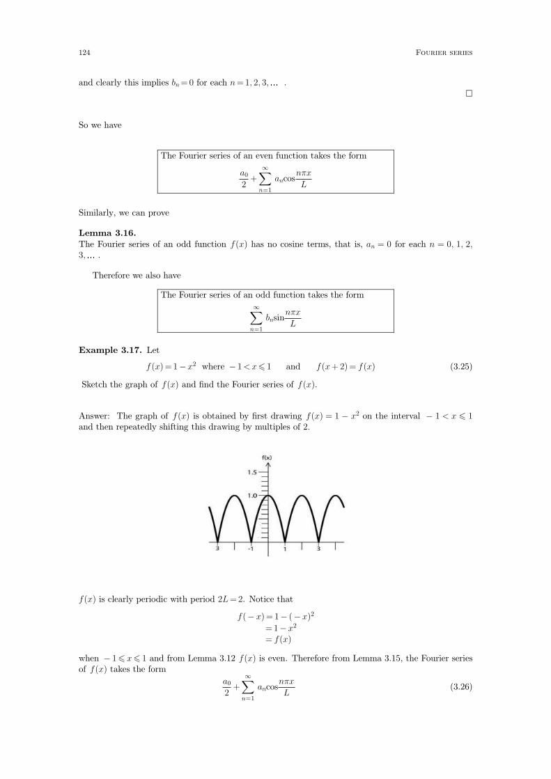
and clearly this implies bn = 0 for each n =1, 2, 3,� .�
So we have
The Fourier series of an even function takes the form
a0
2+∑
n=1
∞ancos
nπx
L
Similarly, we can prove
Lemma 3.16.The Fourier series of an odd function f(x) has no cosine terms, that is, an = 0 for each n = 0, 1, 2,3,� .
Therefore we also have
The Fourier series of an odd function takes the form
∑
n=1
∞bnsin
nπx
L
Example 3.17. Let
f (x)= 1−x2 where − 1< x6 1 and f(x+ 2) = f(x) (3.25)
Sketch the graph of f(x) and find the Fourier series of f(x).
Answer: The graph of f(x) is obtained by first drawing f(x) = 1 − x2 on the interval − 1 < x 6 1and then repeatedly shifting this drawing by multiples of 2.
f(x) is clearly periodic with period 2L =2. Notice that
f(− x)= 1− (−x)2
=1−x2
= f(x)
when − 1 6 x 6 1 and from Lemma 3.12 f(x) is even. Therefore from Lemma 3.15, the Fourier seriesof f(x) takes the form
a0
2+∑
n=1
∞ancos
nπx
L(3.26)
124 Fourier series

that is, bn = 0 when n = 1, 2, 3,� . We use Euler’s formula to determine an. Split the case of an intotwo subcases n= 0 and n = 1, 2,�
a0 =1
L
∫
−L
L
(1− x2) cos0πx
Ldx
=1
1
∫
−1
1
(1−x2)dx as L =1
=
[
x− x3
3
]
−1
1
=4
3
Now determine the an when n =1, 2,�an =
1
L
∫
−L
L
(1− x2) cosnπx
Ldx
=1
1
∫
−1
1
(1− x2) cosnπx
1dx
=
∫
−π
π
(1−x2) cosnπx dx
Integrating by parts withv =1−x2 du = cosnπxdx
dv =− 2x dx u=sinnπx
nπgives
an =
[
(1−x2) sinnπx
nπ
]
−1
1
−∫
−1
1
− 2x sinnπx
nπdx
=0 +
∫
−1
1 2x sinnπx
nπdx
Integrating by parts again with
v = 2x du=sinnπx
nπdx
dv =2 dx u=− cosnπx
n2π2gives
an =
∫
−1
1 2x sinnπx
nπdx
=
[
− 2x cosnπx
n2π2
]
−1
1
−∫
−1
1
− 2cosnπx
n2π2dx
=
[
− 2x cosnπx
n2π2
]
−1
1
+
[
2sinnπx
n3π3
]
−1
1
=− 2cosnπ
n2π2−(
− 2(− 1) cos (−nπ )
n2π2
)
+2sinnπ
n3π3− 2sin (−nπ)
n3π3
and recall when n is an integer
expression value
sinnπ 0
sin (−nπ) 0
cosnπ (− 1)n
cos (−nπ) (− 1)n
and therefore
an =− 4(− 1)n
n2π2when n =1, 2,�
Hence the Fourier series of f(x) is
2
3+∑
n=1
∞ − 4(− 1)n
n2π2cosnπx.
3.3 Even and odd functions 125

3.4 Half range expansions
Let a function f(x) be defined on an interval 0 6 x 6 L. We want to be able to represent f(x) bytwo types of Fourier series – a Fourier series that consists of cosine terms only or a Fourier seriesthat consists of sine terms only.3.5 Essentially, this may be done because we only want the Fourierseries to represent the function for half of the period −L6 x 6L.
Example 3.18. Let f(x) = x on the interval 0 6 x 6 π. Then we will show in Example 3.24 that wecan represent this function f(x) by a Fourier series that consists of cosine terms only, which in thiscase is
x =π
2+
2
π
∑
n=1
∞ (
(− 1)n − 1
n2
)
cosnx
and this equality holds when 0 6 x 6 π. We can also represent f(x) by a Fourier series that consistsof sine terms only, which in this case is
x =2∑
n=1
∞(− 1)n+1
nsinnx
and this equality holds when 06 x <π.
Definition 3.19.
i. A Fourier series that consists of cosine terms only is called a Fourier cosine series.
ii. A Fourier series that consists of sine terms only is called a Fourier sine series.
Hence, given a function f(x) defined on an interval 0 6 x 6 L, we want to be able to represent f(x)by either a Fourier cosine series or a Fourier sine series.
Recall from Lemma 3.15 that the Fourier series of an even function consists of cosine terms only, inother words, the Fourier series of an even function is a Fourier cosine series. Also recall from Lemma3.16 that the Fourier series of an odd function is a Fourier sine series. We use these facts to obtainour desired representation of f(x) by either a Fourier cosine series or a Fourier sine series.
We obtain the representation of f(x) by a Fourier cosine series by first constructing an evenperiodic function that is equal to f(x) on the interval 0 6 x 6 L. Such a function is called an evenperiodic extension of f(x). Similarly we obtain the representation of f(x) by a Fourier sine seriesby constructing an odd periodic function that is equal to f(x) on the interval 0 6 x 6 L. In thiscase, such a function is called an odd periodic extension of f(x).
Definition 3.20. Let a function f(x) be defined on an interval 06x 6 L. Then
i. the function defined as
E(x)=
{
f(x) 0 6x 6 L
f(−x) −L < x < 0, E(x +2L) =E(x)
is the even periodic extension of f(x) of period 2L.
ii. the function defined as
O(x)=
{
f(x) 06 x6 L
− f(− x) −L <x < 0, O(x +2L)= O(x)
is the odd periodic extension of f(x) of period 2L.
3.5. We will use this when solving partial differential equations.
126 Fourier series

Example 3.21. Let f(x)= x on the interval 06x 6 π. Then
i. the even periodic extension of f(x) is
E(x) =
{
x 06 x 6π
− x − π <x < 0, E(x+ 2π)=E(x)
and from the graph of E(x)
we see that E(x) is an even periodic function of period 2π. Also note that
E(x) = f(x) when 06 x6 π .
ii. the odd periodic extension of f(x) is
O(x) =
{
x 06 x6 π
− (−x) − π <x < 0, O(x+ 2π)=O(x)
and from the graph of O(x)
we see that O(x) is an even periodic function of period 2π. Also note that
O(x)= f(x) when 0 6x 6π .
We now define the half-range expansions of a function f(x).
Definition 3.22. Let f(x)be defined on an interval 06x 6 L.
i. The Fourier series of the even periodic extension E(x) of f(x) is called the cosine half-range expansion of f (x) or Fourier cosine series of f(x).
ii. The Fourier series of the odd periodic extension O(x) of f(x) is called the sine half-rangeexpansion of f(x) or Fourier sine series of f(x).
3.4 Half range expansions 127
We explain the idea of Definition 3.22. Consider the case of the cosine half-range expansion of f(x).Recall from Theorem 3.8, that under certain conditions, the Fourier series of any periodic functiong(x) is equal to g(x). As E(x) is, by definition a periodic function, the Fourier series of the evenperiodic extension E(x) is equal to E(x) on the interval −L 6 x 6 L and hence the Fourier series ofthe even periodic extension E(x) is equal to f(x) on the interval 06 x 6L as
E(x) = f(x) when 06 x6 L.
As E(x) is even, its Fourier series consist of cosine terms only. Summarizing, the Fourier series ofthe even periodic extension E(x) is a cosine series that is equal to f(x)3.6 on the interval 06x 6 L.
By a similar reasoning, the Fourier series of the odd periodic extension O(x) is a sine series that isequal to f(x) on the interval 06 x <L.
The following result gives formulae for the cosine and sine half-range expansions of a function.
Lemma 3.23. Let f(x) be defined on an interval 06 x 6L. Then
i. the cosine half-range expansion of f(x) is given by
a0
2+∑
n=1
∞ancos
nπx
Lwhere
an =2
L
∫
0
L
f(x)cosnπx
Ldx where n = 0, 1, 2, 3,�
ii. the sine half-range expansion of f(x) is given by
∑
n=1
∞bnsin
nπx
Lwhere
bn =2
L
∫
0
L
f(x)sinnπx
Ldx where n= 1, 2, 3,�
Proof. i. By definition, the cosine half-range expansion of f(x) is the Fourier series of the evenperiodic extension E(x) of f(x). As E(x) is an even function, by Lemma 3.15 the Fourier series ofE(x) consists of cosine terms only and hence is of the form
a0
2+∑
n=1
∞ancos
nπx
Lwhere
an =1
L
∫
−L
L
E(x)cosnπx
Ldx
for n =0, 1, 2, 3,� . But we know that
E(x)=
{
f(x) 06 x 6L
f(− x) −L <x < 0
and so we may determine an directly from f(x):
an =1
L
∫
−L
L
E(x)cosnπx
Ldx
=1
L
(
∫
−L
0
E(x)cosnπx
Ldx +
∫
0
L
E(x)cosnπx
Ldx
)
=1
L
(
∫
−L
0
f(− x)cosnπx
Ldx+
∫
0
L
f(x)cosnπx
Ldx
)
3.6. provided f(x) is continuous on the interval 0 6x6 L, which we will assume in this class.
128 Fourier series

Using the trigonometry identity cos(− x)= cosx we have that
∫
−L
0
f(−x)cosnπx
Ldx =
∫
−L
0
f(− x)cos(
− nπx
L
)
dx
=−∫
L
0
f(u)cos(
nπu
L
)
du by the substitution u =−x
=
∫
0
L
f(u)cos(
nπu
L
)
du
=
∫
0
L
f(x)cosnπx
Ldx asu is dummyvariable
and therefore
an =1
L
(
∫
−L
0
f(−x)cosnπx
Ldx +
∫
0
L
f(x)cosnπx
Ldx
)
=1
L
(
∫
0
L
f(x)cosnπx
Ldx +
∫
0
L
f(x)cosnπx
Ldx
)
=2
L
∫
0
L
f(x)cosnπx
Ldx
which is our desired result.
The proof of ii) is similar to that of i).
�
Example 3.24. Find the
i. cosine half-range expansion
ii. sine half-range expansion
of the function f(x)= x on the interval 0 6x 6 π.
Answer:
i. In this case L = π. From the formulae in Lemma 3.23 the cosine half-range expansion of f(x)is given by
a0
2+∑
n=1
∞ancosnx
where
an =2
π
∫
0
π
f(x)cosnx dx
=2
π
∫
0
π
x cosnx dx
Split into the case of n =0
a0 =2
π
∫
0
π
x dx= π
and the case of n =1, 2,�an =
2
π
∫
0
π
x cosnx dx
=2
π
([
x sinnx
n
]
0
π
−∫
0
π sinnx
ndx
)
=2
π
([
x sinnx
n
]
0
π
+[ cosnx
n2
]
0
π)
=2
π
(
(− 1)n
n2− 1
n2
)
3.4 Half range expansions 129

and therefore the cosine half-range expansion of f(x) is
π
2+
2
π
∑
n=1
∞ (
(− 1)n − 1
n2
)
cosnx .
ii. From the formulae in Lemma 3.23 the sine half-range expansion of f (x) is given by
∑
n=1
∞bnsinnx
where
bn =2
π
∫
0
π
f(x)sinnx dx
=2
π
∫
0
π
x sinnx dx
=2
π
(
[
− x cosnx
n
]
0
π
+
∫
0
π cosnx
ndx
)
=2
π
(
[
− x cosnx
n
]
0
π+
[
sinnx
n2
]
0
π)
=2(− 1)n+1
n
and therefore the sine half-range expansion of f(x) is
2∑
n=1
∞(− 1)n+1
nsinnx .
130 Fourier series

Chapter 4
Partial Differential Equations
4.1 Definitions
Definition 4.1. An equation involving one or more partial derivatives of an unknown function oftwo or more variables is called a partial differential equation or p.d.e. . The unknown functionis called the dependent variable. The order of the highest derivative is called the order of thepartial differential equation.
Example 4.2.
i.∂u
∂x=
∂u
∂tis a first order p.d.e.
ii.∂2u
∂x2=
∂u
∂tis a second order p.d.e.
Definition 4.3. A partial differential equation is said to be linear if it is of first degree in theunknown function and its partial derivatives.
Example 4.4.
i.∂u
∂x=
∂u
∂t,
∂2u
∂x2=
∂u
∂t,
∂2u
∂x2+
∂2u
∂t2=0 are each linear p.d.e.
ii.
(
∂u
∂x
)2=
∂u
∂t,
∂u
∂x.∂u
∂t=
∂2u
∂x2are each non-linear p.d.e.
iii. Let u(x, t) be a function of the two variables. Then the general form of a second order linearp.d.e. is
a(x, t)∂2u
∂x2+ b(x, t)
∂2u
∂t2+ c(x, t)
∂2u
∂x∂t+ d(x, t)
∂2u
∂t∂x+ e(x, t)
∂u
∂x+ f(x, t)
∂u
∂t+ g(x, t)u =h(x, t)
where a, b, c, d, e, f , g and h are given functions of x and t.
Definition 4.5. If each term of a partial differential equation contains the dependent variable or itspartial derivatives then the equation is said to be homogeneous, otherwise it is said to be inho-mogeneous.
Example 4.6.
i.∂2u
∂x2+
∂2u
∂t2=0 is a homogeneous p.d.e.
ii.∂2u
∂x2+
∂2u
∂t2=x2t is an inhomogeneous p.d.e.
131

Consider a function u(x, y) of the two independent variables x and y. The domain of the functionu(x, y) will be a subset of the xy-plane. For example the real-valued function
u(x, y)= 1− (x2 + y2)√
has domain equal to
{(x, y)|x2 + y2 6 1}which is a closed disc of radius 1:
The closed disc above is an example of a subset in the space of independent variables x andy of the function u(x, y). Note in this example, the space of independent variables x and y is simplythe xy-plane.
Definition 4.7.
A solution of a partial differential equation in a subset R of the space of independent variablesis a function for which all the partial derivatives that appear in the equation exist and satisfies theequation everywhere in R.
Example 4.8.
i. Show that the function u(x, y) = x2 − y2 is a solution of the p.d.e.∂2u
∂x2+
∂2u
∂y2= 0 in the set
R=xy-plane.
Answer: When u(x, y) =x2− y2, the second partial derivatives∂2u
∂x2and
∂2u
∂y2are
∂2u
∂x2=2
∂2u
∂y2=− 2 (4.1)
and so for u(x, y)=x2− y2
∂2u
∂x2+
∂2u
∂y2= 2 + (− 2)
=0
and notice that the second partial derivatives in (4.1) exist for all points in the xy-plane andalso these second partial derivatives satisfy the p.d.e for all points in the xy-plane. Therefore,
by Definition 4.7, u(x, y) = x2 − y2 is a solution of the p.d.e.∂2u
∂x2+
∂2u
∂y2= 0 at each point (x,
y) in the xy-plane.
ii. Show that the function u(x, y) = ln(x2 + y2) is a solution of the p.d.e.∂2u
∂x2+
∂2u
∂y2= 0 in the
set R = {xy-plane − (0, 0)}, in other words, u(x, y) = ln(x2 + y2) is a solution of the givenp.d.e. at all points on the xy-plane except at the origin.
132 Partial Differential Equations

Answer: When u(x, y) = ln(x2 + y2), the second partial derivatives∂2u
∂x2and
∂2u
∂y2are
∂2u
∂x2=
2y2− 2x2
(x2 + y2)2
∂2u
∂y2=
2x2− 2y2
(x2 + y2)2(4.2)
and so for u(x, y) = ln(x2 + y2),
∂2u
∂x2+
∂2u
∂y2=
(
2y2− 2x2
(x2 + y2)2
)
+
(
2x2− 2y2
(x2 + y2)2
)
=0
however, notice that the second partial derivatives in (4.2) exists for all points except when
(x, y) = (0, 0), therefore by Definition 4.7, u(x, y) = ln(x2 + y2) is a solution of the p.d.e.∂2u
∂x2+
∂2u
∂y2=0 at each point (x, y) in the xy-plane except when (x, y) = (0, 0).
Theorem 4.9. (Superposition principle I) If u1 and u2 are solutions of a linear homogeneouspartial differential equation in some subset R in the space of independent variables then, for anyscalars c1 and c2
u= c1u1 + c2u2
is also a solution of that partial differential equation in the subset R.
Proof. (Not required). �
Example 4.10. From Example 4.8 we have that
u1 = x2− y2 and u2 = ln(x2 + y2)
are solutions of the p.d.e.∂2u
∂x2+
∂2u
∂y2= 0 in the set R= {xy-plane− (0, 0)}. Therefore by the Super-
position principle I
u = 15(x2− y2)+ 9ln(x2 + y2)
is a solution of∂2u
∂x2+
∂2u
∂y2=0 in the set R= {xy-plane− (0, 0)}.
We shall see later that we will usually obtain an infinite set of solutions u1, u2, u3,� to a given linearhomogeneous p.d.e. . The following theorem states, that under certain conditions, the sum of suchan infinite set of solutions is also a solution.
Theorem 4.11. (Superposition Principle II) If each function of an infinite set u1, u2, u3, � is asolution of a linear homogeneous partial differential equation in some subset R in the space of inde-pendent variables then the function
u=∑
n=1
∞cnun = c1u1 + c2u2 +� (4.3)
is also a solution of that partial differential equation in the subset R provided the series (4.3) con-verges at each point in R .
Proof. (Not required). �
4.1 Definitions 133

Note 4.12. In this class, we shall use a method of solving p.d.e. that determine constants cn thatwill ensure that the series
u=∑
n=1
∞cnun = c1u1 + c2u2 +�
converges. This method is based on Theorem 3.8 on page 118. We will not directly test for conver-gence, our method will automatically guarantee convergence.
Example 4.13. One can check each of the functions
e−tcosx, e−9tcos 3x, e−25tcos 5x,� , e−(2n+1)2tcos(2n +1)x,�is a solution of
∂u
∂t=
∂2u
∂x2(4.4)
in the subset R= {(x, t)|t> 0}. It is possible to prove 4.1that the series
∑
n=1
∞1
(2n− 1)2e−(2n−1)2tcos(2n− 1)x
= e−tcosx+1
9e−9tcos 3x +
1
25e−25tcos 5x+� (4.5)
converges at each point in the subset R = {(x, t)|t > 0}, therefore by the Superposition Principle IIthe series (4.5) is a solution of the partial differential equation (4.4) in the subset R= {(x, t)|t> 0}.
We shall be interested in the following linear homogeneous partial differential equation of the secondorder:
∂u
∂t= c2∂2u
∂x2one dimensional heat equation
∂2u
∂t2= c2∂2u
∂x2one dimensional wave equation
∂2u
∂x2+
∂2u
∂x2= 0 two dimensional Laplace’s equation
∂2u
∂r2+
1
r
∂u
∂r+
1
r2
∂2u
∂θ2= 0 Laplace’s equation in polar coordinates
∂2u
∂r2+
1
r
∂u
∂r+
1
r2
∂2u
∂θ2+
∂2u
∂z2= 0 Laplace’s equation in cylindrical coordinates
1
r2
(
∂
∂r
(
r2∂u
∂r
)
+1
sin φ
∂
∂φ
(
sin φ∂u
∂φ
)
+1
sin2 φ
∂2u
∂θ2
)
= 0 Laplace’s equation in spherical coordinates
4.1. A direct proof of this convergence is beyond the scope of this class
134 Partial Differential Equations

4.2 The Heat Equation
4.2.1 A derivation of the heat equation
We illustrate how the one-dimensional heat equation
∂u
∂t= c2∂
2u
∂x2(4.6)
models a certain physical situation.
Consider a bar of metal of length L. We wish to describe how the temperature of this barchanges with time t. To simplify our model we assume that our rod is one-dimensional, that is, ithas no thickness. Assume also that the metal bar is insulated along the sides. We place our bar oflength L along the x-axis as follows.
Notice that as the bar is insulated along the sides, heat may escape the bar only at points
x =0 and x=L,
that is, heat can only escape at the ends of the bar.
Let u(x, t) denote the temperature of the bar at a point x and at time t. Note that the domainof this temperature function u(x, t) is
06 x6 L and 0 6 t <∞.
We wish to model the following problem. The metal bar has an initial temperature distribution,which is not necessarily uniform along the bar. That is, at time t = 0, the bar has a temperaturethat varies along the length of the bar, so this initial temperature distribution varies with x and canbe stated as
u(x, 0)= f(x) where 0 6x 6L (4.7)
where the function f(x) describes the initial temperature distribution along the bar. The equation(4.7) is an example of an initial condition.
For simplicity, we assume in this particular problem that the ends of the bar will be at zero tem-perature for all time t> 0. This may be stated as
u(0, t)= 0 for any t> 0 (4.8)
u(L, t) = 0 for any t> 0 (4.9)
Equations (4.8) and (4.9) are examples of boundary conditions.
4.2 The Heat Equation 135

Summarizing so far, our physical problem is as follows. We have a bar that has aninitial temperature that is given by equation (4.7). We insulate the bar along thesides and allow the heat to escape from the ends. Therefore the temperature of thebar will change with time. We wish to find the temperature function u(x, t) thatdescribes this change and will show that such a u(x, t) will be a solution of the heatequation (4.6).
To derive the heat equation, we consider a small segment of the metal bar that lies between thepoint x and x + ∆x where ∆x represents a small positive number. We represent this segment by thegrey area in the following diagram of the metal bar.4.2
As the bar is insulated along the sides, the heat flow out of the segment is only in the indicateddirection of the arrows A and B.
Recall that heat flows from one point to another point if these points are at different tempera-tures. Now the temperature at a point x on our metal bar at time t is given by the function
u(x, t).
Note that a difference in temperature u(x, t) from one point to the next is measured by the changeof the function u(x, t) with respect to x. By the definition of partial derivatives, such a change in u
with respect to x is given by the partial derivative∂u
∂x. And as heat flow occurs when we have tem-
perature change, we expect that heat flow at the point x + ∆x on the metal bar at time t should be
proportional to the partial derivative∂u
∂x(x + ∆x, t). This is in fact true – the Law of Heat Con-
duction from physics tells us that the rate of heat flow at the point x + ∆x at time t (indicated byarrow A) is given by
− k∂u
∂x(x+ ∆x, t) (4.10)
where k is the thermal conductivity of the metal. The −8 sign′ appears in (4.10) because heat flows
from points of high temperature to points of low temperature while∂u
∂xis positive when temperature
increases with distance x.
Similarly the rate of heat flow at the point x at time t (as indicated by arrow B) is given by
k∂u
∂x(x, t). (4.11)
Notice that the sign of (4.11) is opposite to that of (4.10) because arrow B points in the oppositedirection of arrow A. Now as heat flows out of the segment only in the direction of arrows A and B,we have that
rate of heat loss in segment= k∂u
∂x(x, t) − k
∂u
∂x(x +∆x, t) (4.12)
4.2. We draw our one dimensional metal bar as having width and height ONLY for illustrative purposes.
136 Partial Differential Equations

We can determine the rate of heat loss in the segment by another means. Recall that the more thetemperature of an object increases, the more heat it will contain. In fact if an object has mass m,specific heat capacity C and temperature T (t) then, also from physics:
rate of heat increase of object=mass× specific heat capacity × rate of temperature increase
=mCdT
dt.
Using the above physical law, it is possible to show4.3 that
rate of heat increase in segment = ρC∂u(ξ, t)
∂t∆x where x 6 ξ 6x +∆x
where ρ is the mass per unit length of the metal bar and C is the specific heat capacity of the metalbar. Therefore
rate of heat loss in segment=− ρC∂u(ξ, t)
∂t∆x where x 6 ξ 6 x+ ∆x (4.13)
and so from equations (4.12) and (4.13) we have
− ρC∂u(ξ, t)
∂t∆x= k
∂u
∂x(x, t) − k
∂u
∂x(x +∆x, t). (4.14)
Rearranging equation (4.14) gives
∂u(ξ, t)
∂t=
k
ρC
(
∂u
∂x(x +∆x, t)− ∂u
∂x(x, t)
∆x
)
(4.15)
and taking the limit of (4.15) as ∆x→ 0 gives
lim∆x→0
∂u(ξ, t)
∂t=
k
ρClim
∆x→0
(
∂u
∂x(x+ ∆x, t)− ∂u
∂x(x, t)
∆x
)
. (4.16)
Now because x 6 ξ 6 x +∆x we have that ξ→x as ∆x→ 0 and therefore
lim∆x→0
∂u(ξ, t)
∂t=
∂u(x, t)
∂t.
By definition of the partial derivative
lim∆x→0
(
∂u
∂x(x +∆x, t)− ∂u
∂x(x, t)
∆x
)
=∂
∂x
(
∂u
∂x(x, t)
)
=∂2u(x, t)
∂x2
and so from equation (4.16) we obtain
∂u(x, t)
∂t=
k
ρC
∂2u(x, t)
∂x2(4.17)
and as k, ρ and C are positive constants we may write equation (4.17) in the standard form of theheat equation
∂u
∂t= c2∂
2u
∂x2
where c is a constant.
4.3. by using a Mean Value theorem to obtain
∫
x
x+∆x
ρC∂u(s, t)
∂tds = ρC
∂u(ξ, t)
∂t∆x where x6 ξ 6x+ ∆x
4.2 The Heat Equation 137

We have shown that the temperature u(x, t) of our metal bar satisifes the partial dif-ferential equation
∂u
∂t= c2∂
2u
∂x2
subject to the initial condition
u(x, 0)= f(x) where 0 6x 6L
and boundary conditionsu(0, t)= 0u(L, t)= 0
where t> 0.
In the next section we give a technique for obtaining a solution of such partial differ-ential equations.
4.2.2 Solution of the heat equation by seperation of variables
We illustrate the use of the seperation of variables technique in the solution of the following one-dimensional heat equation.
Example 4.14. Let u(x, t) denote the temperature of a thin metal bar of length 1 that is insulatedalong the sides. Let the temperature along the length of the bar at time t= 0 be given by
u(x, 0)=4x(1−x) where 06 x6 1.
The ends of the bar are kept at a constant temperature of 0, that is
u(0, t)= 0u(1, t)= 0
where t> 0.
Determine the temperature u(x, t) of the bar by solving the following heat equation
∂u
∂t= c2∂
2u
∂x2(4.18)
where c is a fixed constant that depends on the physical properties of the bar.
Answer: The method of seperation of variables begins with the assumption that our solution u(x, t)takes the form
u(x, t)= X(x)T (t), (4.19)
that is, the function of two variables u(x, t) is ‘seperated’ into a product of a single variable functionX(x) and a single variable function T (t). Substituting the solution (4.19) into heat equation (4.18)gives
∂
∂t(X(x)T (t))= c2 ∂2
∂x2(X(x)T (t)). (4.20)
Recall that to differentiate partially with respect to t, we treat the variable x as a constant. There-fore, when differentiating X(x)T (t) with respect to t, the function X(x) behaves as a constant andwe have
∂
∂t(X(x)T (t)) =X(x)T ′(t)
where T ′(t) denotes the (ordinary) derivative of T (t). Similarly
∂2
∂x2(X(x)T (t))= X ′′(x)T (t)
138 Partial Differential Equations
and so from equation (4.20) we have
X(x)T ′(t)= c2X ′′(x)T (t)
⇒ T ′(t)c2T (t)
=X ′′(x)
X(x)(4.21)
The left sideT ′(t)
c2T (t)of equation (4.21) is a function of the variable t; the right side
X ′′(x)
X(x)of (4.21) is
a function of a different variable x. IfT ′(t)c2T (t)
� constant
then the value of the functionT ′(t)
c2T (t)will vary with t. Similarly, if
X ′′(x)
X(x)� constant
then the value of the functionX ′′(x)
X(x)will vary with x and, in fact, equation (4.21) will be false
because we can choose values of t and x such thatT ′(t)
c2T (t)and
X ′′(x)
X(x)take different values. The only
way for equation (4.21) to hold is ifT ′(t)
c2T (t)and
X ′′(x)
X(x)are both constant functions and are equal to
the same constant k. So we have
T ′(t)c2T (t)
=X ′′(x)
X(x)= k. (4.22)
We now need to determine if this constant k is zero, positive or negative. That is, we need to deter-mine if k =0, a2 or − a2 where a� 0. Using the boundary conditions
u(0, t)= 0u(1, t)= 0
where t> 0 (4.23)
we show that the only non-zero solutions of the heat equation (4.18) with these particular boundaryconditions 4.4occurs when k =− a2 :
k = 0
If k =0 then from equation (4.22) we obtain two ordinary differential equations
T ′(t)= 0
X ′′(x) = 0.
Solving these gives
T (t)= A′
X(x)=B ′x +C ′ (4.24)
where A′, B ′ and C ′ are constants.
Substituting equations (4.24) into equation (4.19) gives
u(x, t)=X(x)T (t)= Ex +F (4.25)
where E =A′B ′ and F = A′C ′.
From the first boundary condition of (4.23) we get
u(0, t) =E(0)+F = 0
⇒ F =0
4.4. In Example 4.15 we will see that the value k = 0 will give a non-zero solution because the boundary conditions of thatexample are different from the boundary conditions of this example.
4.2 The Heat Equation 139

The second boundary condition gives
u(1, t)= E(1) + 0 =0
⇒ E = 0
As E = F = 0 in (4.25), we have that the solution (4.25) of our heat equation corresponding to k = 0must be identically equal to zero.
k = a2
If k = a2 then from equation (4.22) we have
X ′′(x)
X(x)= a2
⇒ X ′′(x)− a2X(x)= 0⇒ X(x)= C cosh (ax)+ D sinh (ax)
where C and D are constants. From equation (4.19) we have
u(x, t)= (C cosh (ax) +D sinh (ax))T (t). (4.26)
From the first boundary condition of (4.23) we get
u(0, t)= (C cosh(0)+D sinh(0))T (t)= 0
⇒ (C(1)+ D(0))T (t)≡ 0
⇒ CT (t)≡ 0
and this implies C =0. The second boundary condition gives
u(1, t)=D sinh(a)T (t)≡ 0 (4.27)
and as sinh a � 0 when a � 0, equation (4.27) implies that D = 0. As C = D = 0, we have that thesolution (4.26) obtained when k = a2 is identically equal to zero.
The last possibility of k = − a2 will lead to non-zero solutions of the heat equation (4.18). Subsi-tuting k =− a2 into equation (4.22) gives
T ′(t)c2T (t)
=X ′′(x)
X(x)=− a2
from which we obtain
T ′(t)+ c2a2T (t)= 0 (4.28)
X ′′(x)+ a2X(x)= 0 (4.29)
and this is the point of the seperation of variables method, the assumption
u(x, t)=X(x)T (t)
converts the partial differential equation
∂u
∂t= c2∂
2u
∂x2
into two ordinary differential equations (4.28) and (4.29) which can be easily solved. By using theD-operator method, the general solution of (4.28) is
T (t) =Ce−c2a2t
and the general solution of (4.29) is
X(x) =D cos(ax) +E sin(ax).
140 Partial Differential Equations

And so we have solutions of the heat equation (4.18) of the form
u(x, t)= e−c2a2t(A cos (ax)+ B sin (ax)) (4.30)
where the arbitrary constants A =CD and B =CE. Note that a is also an arbitrary constant.
We now impose the boundary conditions on equation (4.30). From the first boundary condition of(4.23) we get
u(0, t)= e−c2a2t(A cos(0)+B sin (0))≡ 0
⇒ Ae−c2a2t≡ 0
⇒ A =0.
Substituting A =0 into (4.30) implies that our solution of the heat equation (4.18) is of the form
u(x, t)=Be−c2a2tsin(ax). (4.31)
Imposing the second boundary condition of (4.23) on equation (4.31) gives
u(1, t) =Be−c2a2tsin(a)≡ 0
⇒ sin(a)= 0
and so the second boundary condition forces
a= kπ where k =1, 2, 3,� (4.32)
(note we do not consider k = 0 as this leads to the zero solution; k =− 1,− 2,� do not give solutionsthat are linearly independent of the solutions corresponding to k = 1, 2, � ). Substituting each ofthese different values of a into equation (4.31) implies that
e−c2π2tsin(πx), e−c2(2π)2tsin(2πx), e−c2(3π)2tsin(3πx),�are each solutions of the heat equation (4.18). So from by the Superposition Principle II on page 133we have that
u(x, t) =∑
n=1
∞bne
−c2(nπ)2tsin(nπx) (4.33)
is a solution of the heat equation (4.18) which, by construction, satisfies the boundary conditions.
Finally, we use the given initial condition
u(x, 0)=4x(1−x) where 06 x 6 1
to determine the constants bn of equation (4.33). Setting t= 0 in (4.33) gives
u(x, 0) =∑
n=1
∞bne
−c2(nπ)20sin(nπx)= 4x(1− x) when 0 6x 6 1
⇒∑
n=1
∞bnsin(nπx)= 4x(1−x) when 06 x 6 1 (4.34)
The left side of equation (4.34) is nothing but a Fourier sine series that represents the function4x(1 − x) on the interval 0 6 x 6 1. Recall that such a sine series is called the sine half-rangeexpansion of the function 4x(1 − x) on the interval 0 6 x 6 1 and from Lemma 3.23 on page 128,the coefficients bn of the left side of (4.34) are given by
bn =2
L
∫
0
L
f(x)sinnπx
Ldx
⇒ bn = 2
∫
0
1
4x(1− x)sin (nπx) dx
4.2 The Heat Equation 141

Integrating by parts with
v = 4x(1− x) du = sin(nπx)dx
dv = (4− 8x) dx u=− cos (nπx)
nπgives
bn =2
[
− 4x(1− x)cos (nπx)
nπ
]
0
1
+2
∫
0
1 (4− 8x)cos (nπx)
nπdx
= 0 +2
∫
0
1 (4− 8x)cos (nπx)
nπdx
Integrating by parts again with
v = (4− 8x) du =cos (nπx)
nπdx
dv =− 8 dx u =sin (nπx)
n2π2
gives
bn =2
[
(4− 8x)sin (nπx)
n2π2
]
0
1
+2
∫
0
1 8sin (nπx)
n2π2dx
= 0 +2
[
− 8cos (nπx)
n3π3
]
0
1
=2
(
− 8(− 1)n
n3π3+
8
n3π3
)
=
0 when n is even
32
n3π3 when n is odd
Substituting these values for bn into (4.33) and writing the odd values of n as 2k + 1 gives our solu-tion
u(x, t)=∑
k=0
∞32
(2k +1)3π3e−c2((2k+1)π)2tsin((2k +1)πx) (4.35)
that satisfies the heat equation (4.18) subject to the given boundary and initial conditions.
In the above problem, the metal bar initially had a non-zero temperature distribution given by theinitial condition
u(x, 0)=4x(1−x) where 06 x 6 1
and the ends of the bar are held at zero temperature. As heat flows from a high temperature to alower temperature, we expect the initial heat contained in the bar to flow out of the bar through theends which are held at zero temperature. Therefore the bar should eventually lose its heat and henceeach point in the bar should have zero temperature. This physical expectation actually agrees withthe solution (4.35) above. First notice that
limt→∞
32
π3e−c2π2tsin(πx)=
(
limt→∞
32
π3e−c2π2t
)
(
limt→∞
sin(πx))
=0.(
limt→∞
sin(πx))
= 0where
limt→∞
e−c2π2t = 0
142 Partial Differential Equations

as the coefficient − c2π2 of t in e−c2π2t is negative. Similarly the limit of each term in the solution(4.35) is zero as each term in
u(x, t)=∑
k=0
∞32
(2k +1)3π3e−c2((2k+1)π)2tsin((2k +1)πx)
=32
π3e−c2π2tsin(πx)+
32
27π3e−c2(2π)2tsin(2πx)+
32
125π3e−c2(3π)2tsin(3πx)+� (4.36)
contains a exponential with a negative coefficient. Therefore we have
limt→∞
u(x, t) = limt→∞
∑
k=0
∞32
(2k +1)3π3e−c2((2k+1)π)2tsin((2k + 1)πx)
= limt→∞
(
32
π3e−c2π2tsin(πx) +
32
27π3e−c2(2π)2tsin(2πx)+
32
125π3e−c2(3π)2tsin(3πx)+� )
= limt→∞
32
π3e−c2π2tsin(πx)+ lim
t→∞
32
27π3e−c2(2π)2tsin(2πx) + lim
t→∞
32
125π3e−c2(3π)2tsin(3πx) +�
= 0 +0 + 0 +�= 0.
and note
limt→∞
u(x, t)= 0
can be interpreted as meaning that the temperature of the bar u(x, t) eventually becomes zero.
4.2.3 The heat equation with insulated ends as boundary conditions
We now consider a similar heat conduction problem in a thin metal bar that is insulated along thesides of the bar. Again we assume the bar has a initial non-zero temperature distribution. However,unlike Example 4.14, we do not hold the ends of the bar at temperature zero. In this case we assumethe ends of the bar to be insulated (so that the bar is entirely insulated). Recall from equation(4.10) on page 136, that the heat flow at point x on the bar is given by
− k∂u
∂x(x, t).
If the ends x = 0 and x = L of a bar of length L are insulated then there is no heat flow at thesepoints and therefore
− k∂u
∂x(0, t)= 0 and − k
∂u
∂x(L, t)= 0,
and hence the insulation of the ends of a bar of length L can be mathematically stated as
∂u
∂x(0, t) = 0
∂u
∂x(L, t)= 0.
(4.37)
The equations (4.37) is another example of boundary conditions.
Example 4.15. Let u(x, t) denote the temperature of a thin metal bar of length π that is insulatedalong the sides. Let the temperature along the length of the bar at time t= 0 be given by
u(x, 0) =1− x
πwhere 06 x6 π.
The ends of the bar are insulated for time t> 0 and therefore
∂u
∂x(0, t)= 0
∂u
∂x(π, t)= 0
where t> 0.
4.2 The Heat Equation 143

Determine the temperature u(x, t) of the bar by solving the following heat equation
∂u
∂t= c2∂
2u
∂x2(4.38)
where c is a fixed constant that depends on the physical properties of the bar.
Answer: We use the method of seperation of variables and therefore assume that our solution u(x, t)takes the form
u(x, t)=X(x)T (t). (4.39)
Substituting the solution (4.39) into heat equation (4.38) gives
∂
∂t(X(x)T (t))= c2 ∂2
∂x2(X(x)T (t))
⇒ X(x)T ′(t) = c2X ′′(x)T (t)
⇒ T ′(t)c2T (t)
=X ′′(x)
X(x)(4.40)
and the only way for equation (4.40) to hold is ifT ′(t)
c2T (t)and
X ′′(x)
X(x)are both constant functions and
are equal to the same constant k. So we have
T ′(t)c2T (t)
=X ′′(x)
X(x)= k (4.41)
where the constant k can be zero, negative or positive, that is
k =0,− a2 or a2
where a� 0. We now use the boundary conditions
∂u
∂x(0, t)= 0
∂u
∂x(π, t)= 0
where t> 0 (4.42)
to show that the only non-zero solutions of the heat equation (4.38) with the boundary conditions(4.42) occur when k =0 and k =− a2.
k = a2
If k = a2 then from equation (4.41) we have
X ′′(x)
X(x)= a2
⇒ X ′′(x)− a2X(x)= 0⇒ X(x)= C cosh (ax)+ D sinh (ax)
where C and D are constants. From equation (4.39) we have
u(x, t)= (C cosh (ax)+D sinh (ax))T (t). (4.43)
which implies∂u
∂x(x, t) = (aC sinh (ax)+ aD cosh (ax))T (t) (4.44)
From the first boundary condition of (4.23) we get
∂u
∂x(0, t) = (aC sinh (0)+ aD cosh (0))T (t)
⇒ (aC(0)+ aD(1))T (t)≡ 0
⇒ a DT (t)≡ 0
144 Partial Differential Equations
and this implies D =0. The second boundary condition gives
∂u
∂x(π, t)= aC sinh(aπ)T (t)≡ 0 (4.45)
and as sinh (aπ) � 0 when a � 0, equation (4.45) implies that C = 0. As C = D = 0, we have that thesolution (4.43) obtained when k = a2 is identically equal to zero.
k = 0
If k =0 then from equation (4.41) we obtain two ordinary differential equations
T ′(t)= 0
X ′′(x) = 0.
Solving these gives
T (t)= A′
X(x)=B ′x +C ′ (4.46)
where A′, B ′ and C ′ are constants.
Substituting equations (4.46) into equation (4.39) gives
u(x, t) =Ex+ F (4.47)
where E =A′B ′ and F = A′C ′. Taking the partial derivative gives
∂u
∂x(x, t)= E (4.48)
From the first boundary condition of (4.42) we get
∂u
∂x(0, t)= E =0.
The second boundary condition also gives
∂u
∂x(π, t)= E =0.
Notice that the boundary conditions (4.42) do not give any information about the constant F inequation (4.47), so it is possible that F � 0, and therefore when k = 0 the heat equation (4.38) mayhave a non-zero solution of the form
u(x, t)=F . (4.49)
k =− a2
The last possibility of k = − a2 will also lead to non-zero solutions. Subsituting k = − a2 into equa-tion (4.41) gives
T ′(t)c2T (t)
=X ′′(x)
X(x)=− a2
from which we obtain the two ordinary differential equations
T ′(t)+ c2a2T (t)= 0 (4.50)
X ′′(x)+ a2X(x) = 0 (4.51)
By using the D-operator method, the general solution of (4.50) is
T (t) =Ce−c2a2t
4.2 The Heat Equation 145

and the general solution of (4.51) is
X(x) =D cos(ax) +E sin(ax).
And so we have solutions of the heat equation of the form
u(x, t)= e−c2a2t(A cos (ax)+ B sin (ax)) (4.52)
where the arbitrary constants A = CD and B = CE. Note that a is also an arbitrary constant. Bytaking the partial derivative of (4.52) we get
∂u
∂x(x, t) = e−c2a2t(− aA sin (ax)+ aB cos (ax)) (4.53)
and we now impose the boundary conditions on equation (4.53). From the first boundary conditionof (4.42) we get
∂u
∂x(0, t)= e−c2a2t(− aA sin(0)+ aB cos (0))≡ 0
⇒ aBe−c2a2t≡ 0
⇒ B =0.
Substituting B =0 into (4.30) implies that the solutions corresponding to k =− a2 is of the form
u(x, t)=Ae−c2a2tcos(ax)
⇒ ∂u
∂x(x, t)= e−c2a2t(− aA sin (ax)) (4.54)
Imposing the second boundary condition of (4.42) on equation (4.54) gives
∂u
∂x(π, t)= e−c2a2t(− aA sin (aπ))≡ 0
⇒ sin(aπ) = 0
and so the second boundary condition forces
a= k where k =1, 2, 3,�(note we do not consider k = 0 as this leads to the zero solution; k =− 1,− 2,� do not give solutionsthat are linearly independent of those corresponding to k = 1, 2, � ). Substituting each of these dif-ferent values of a into equation (4.53) implies that
e−c2tcos(x), e−c222tcos(2x), e−c232tcos(3x) ,�are each solutions of the heat equation with the given boundary conditions. So from by the Superpo-sition Principle II on page 133 we have that
u(x, t)=∑
n=1
∞ane
−c2n2tcos(nx) (4.55)
is a solution of the heat equation that corresponds to k =− a2. From equation (4.49)
u(x, t)=a0
2(4.56)
is also a solution of the heat equation (that corresponds to k = 0) where we rename the constant F
asa0
2. Since both (4.55) and (4.56) are solutions, by the Superposition Principle their sum
u(x, t) =a0
2+∑
n=1
∞ane
−c2n2tcos(nx) (4.57)
is a solution of the heat equation.
146 Partial Differential Equations

Finally, we use the given initial condition
u(x, 0)=1− x
πwhere 0 6x 6 π
to determine the constants an of equation (4.57). Setting t=0 in (4.57) gives
u(x, 0)=a0
2+∑
n=1
∞ane
−c2(nπ)20cos(n x)= 1− x
πwhen 06 x6 π
⇒ a0
2+∑
n=1
∞ancos(n x)= 1− x
πwhen 06x 6 π (4.58)
The left side of equation (4.34) is nothing but a Fourier cosine series that represents the function1− x
πon the interval 0 6 x 6 π. Such a cosine series is called the cosine half-range expansion of
the function 1 − x
πon the interval 0 6 x 6 π and from Lemma 3.23 on page 128, the coefficients an
of the left side of (4.58) are given by
an =2
L
∫
0
L
f(x)cosnπx
Ldx where n =0, 1, 2,�
⇒ an =2
π
∫
0
π (
1− x
π
)
cos (nx) dx where n = 0, 1, 2,�When n =0 we have
a0 =2
π
∫
0
π (
1− x
π
)
dx
=2
π
[
x− x2
2π
]
0
π
=1
When n =1, 2,� then applying integration by parts to
an =2
π
∫
0
π (
1− x
π
)
cos (nx) dx
with
v =1− x
πdu= cos(nx)dx
dv =− 1
πdx u=
sin (nx)
ngives
an =2
π
[
(
1− x
π
)sin (nx)
n
]
0
π
+2
π2
∫
0
π sin (nx)
ndx
=0− 2
π2
[
cos (nx)
n2
]
0
π
=
0 when n is even4
n2π2 when n is odd
Substituting these values for an into (4.58) and writing the odd values of n as 2k + 1 gives our solu-tion
u(x, t)=1
2+∑
k=0
∞4
(2k +1)2π2e−c2(2k+1)2tcos((2k +1)x) (4.59)
that satisfies the heat equation (4.38) subject to the given boundary and initial conditions.
In the previous problem, the metal bar initially had a non-zero temperature distribution given bythe initial condition
u(x, 0) =1− x
πwhere 06 x6 π.
4.2 The Heat Equation 147

At time t = 0 the ends of the bar were insulated. As the bar is also insulated along the sides, thisimplies that the bar is entirely insulated for time t > 0. Hence we expect no heat loss from the bar;furthermore we expect the initial heat of the bar to eventually distribute itself evenly throughout thelength of the bar. So we expect as time t→∞, that each point of the bar should have the same tem-perature. This physical expectation agrees with the solution (4.59) above, because
limt→∞
u(x, t) = limt→∞
(
1
2+∑
k=0
∞4
(2k +1)2π2e−c2(2k+1)2tcos((2k + 1)x)
)
=1
2+ lim
t→∞
4
π2e−c2tcos(x)+ lim
t→∞
4
32π2e−9c2tcos(3x) + lim
t→∞
4
52π2e−25c2tcos(5x)+�
=1
2+ 0 +0 + 0 +�
=1
2
and note
limt→∞
u(x, t) =1
2
can be interpreted as meaning that the temperature of each point on the bar u(x, t) eventually
becomes equal to1
2. Also notice that
1
2is the average of the initial temperature distribution
u(x, 0)=1− x
πwhere 0 6x 6 π
as
1
2=
∫
0
π(
1− x
π
)
dx
length of bar=
∫
0
π(
1− x
π
)
dx
π.
4.2.4 The heat equation with nonhomogeneous boundary conditions
The boundary conditions of the Example 4.14
u(0, t)= 0u(1, t)= 0
where t> 0
and the boundary conditions of Example 4.15
∂u
∂x(0, t)= 0
∂u
∂x(π, t)= 0
where t> 0
are examples of homogeneous boundary conditions.
Definition 4.16. If the boundary conditions of the one-dimensional heat equation
∂u
∂t= c2∂
2u
∂x2where 0 <x <a and t > 0
can be written in the form
αu(0, t)+ β∂u
∂x(0, t) = 0
γu(a, t)+ δ∂u
∂x(a, t)= 0
where t> 0
where α, β, γ and δ are constants, then such boundary conditions are said to be homogeneous.Otherwise, the boundary conditions are called nonhomogeneous.
148 Partial Differential Equations
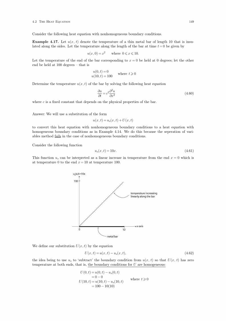
Consider the following heat equation with nonhomogeneous boundary conditions.
Example 4.17. Let u(x, t) denote the temperature of a thin metal bar of length 10 that is insu-lated along the sides. Let the temperature along the length of the bar at time t=0 be given by
u(x, 0)= x2 where 06 x6 10.
Let the temperature of the end of the bar corresponding to x = 0 be held at 0 degrees; let the otherend be held at 100 degrees – that is
u(0, t) = 0u(10, t)= 100
where t> 0
Determine the temperature u(x, t) of the bar by solving the following heat equation
∂u
∂t= c2∂
2u
∂x2(4.60)
where c is a fixed constant that depends on the physical properties of the bar.
Answer: We will use a substitution of the form
u(x, t) =us(x, t) +U(x, t)
to convert this heat equation with nonhomogeneous boundary conditions to a heat equation withhomogeneous boundary conditions as in Example 4.14. We do this because the seperation of vari-ables method fails in the case of nonhomogeneous boundary conditions.
Consider the following function
us(x, t)= 10x. (4.61)
This function us can be interpreted as a linear increase in temperature from the end x = 0 which isat temperature 0 to the end x= 10 at temperature 100.
We define our substitution U(x, t) by the equation
U(x, t) =u(x, t)− us(x, t), (4.62)
the idea being to use us to ‘subtract’ the boundary condition from u(x, t) so that U(x, t) has zerotemperature at both ends, that is, the boundary conditions for U are homogeneous:
U(0, t) =u(0, t)−us(0, t)= 0− 0
U(10, t)= u(10, t)− us(10, t)= 100− 10(10)
where t> 0
4.2 The Heat Equation 149

The function us was also chosen to be a solution of the heat equation. By differentiating (4.61) par-tially it is easy to see that
∂us
∂t= c2∂
2us
∂x2(4.63)
and because (4.63) holds, we have that U(x, t) also satisfies the heat equation: substituting
u(x, t) =U(x, t) +us(x, t)
into∂u
∂t= c2∂
2u
∂x2
gives∂(U +us)
∂t= c2∂
2(U + us)
∂x2
⇒ ∂U
∂t+
∂us
∂t= c2∂
2us
∂x2+ c2∂
2U
∂x2(4.64)
and subtracting (4.63) from (4.64) gives
∂U
∂t= c2∂
2U
∂x2. (4.65)
(If the function us were not a solution of the heat equation, then the partial differential equation inU obtained would not take the standard form of the heat equation (4.65) ).
From equation (4.62) we can also determine the initial condition for U(x, t)
u(x, 0)= 10x +U(x, 0)
⇒ U(x, 0)=x2− 10x for 06x 6 10.
Therefore we have that the substitution (4.62) converts the heat equation
∂u
∂t= c2∂
2u
∂x2
subject to the nonhomogeneous boundary conditions
u(0, t) = 0u(10, t)= 100
where t> 0
and initial condition
u(x, 0)= x2 where 06 x6 10
to another heat equation
∂U
∂t= c2∂
2U
∂x2
subject to the homogeneous boundary conditions
U(0, t) = 0U(10, t)= 0
where t> 0 (4.66)
and initial condition
U(x, 0) =x2− 10x where 06 x6 10
150 Partial Differential Equations
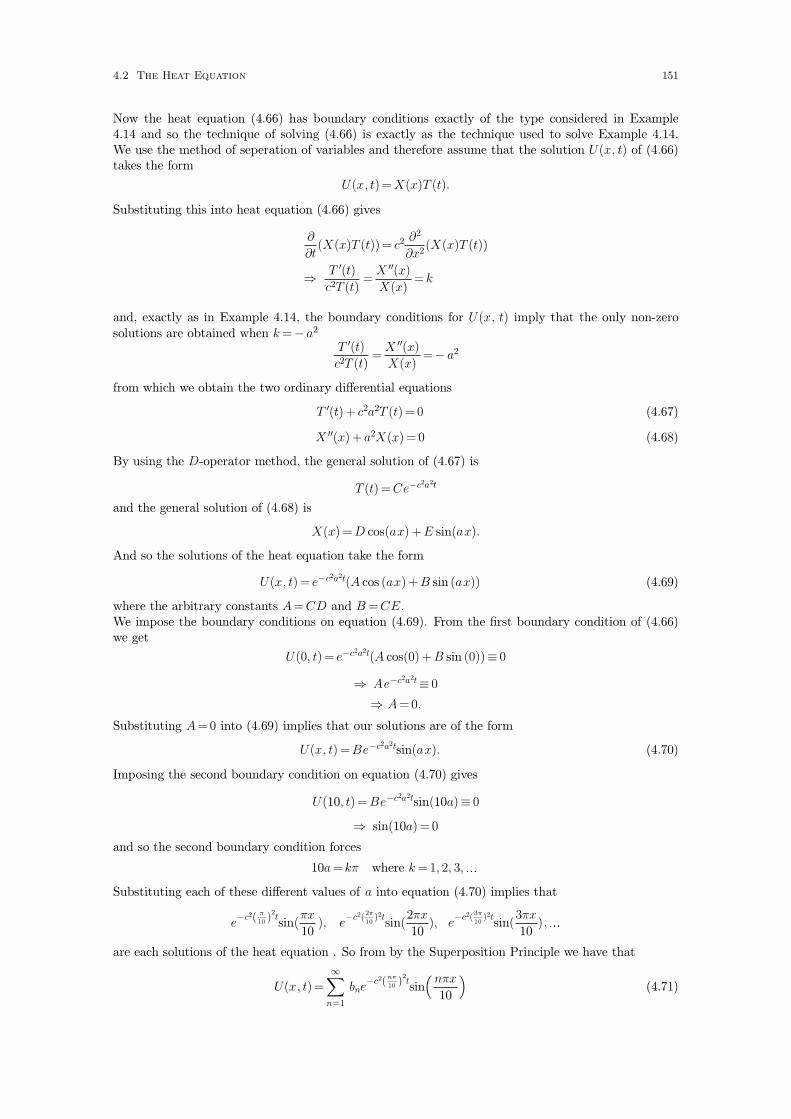
Now the heat equation (4.66) has boundary conditions exactly of the type considered in Example4.14 and so the technique of solving (4.66) is exactly as the technique used to solve Example 4.14.We use the method of seperation of variables and therefore assume that the solution U(x, t) of (4.66)takes the form
U(x, t) =X(x)T (t).
Substituting this into heat equation (4.66) gives
∂
∂t(X(x)T (t))= c2 ∂2
∂x2(X(x)T (t))
⇒ T ′(t)c2T (t)
=X ′′(x)
X(x)= k
and, exactly as in Example 4.14, the boundary conditions for U(x, t) imply that the only non-zerosolutions are obtained when k =− a2
T ′(t)c2T (t)
=X ′′(x)
X(x)=− a2
from which we obtain the two ordinary differential equations
T ′(t)+ c2a2T (t)= 0 (4.67)
X ′′(x)+ a2X(x) = 0 (4.68)
By using the D-operator method, the general solution of (4.67) is
T (t) =Ce−c2a2t
and the general solution of (4.68) is
X(x) =D cos(ax) +E sin(ax).
And so the solutions of the heat equation take the form
U(x, t)= e−c2a2t(A cos (ax)+B sin (ax)) (4.69)
where the arbitrary constants A =CD and B =CE.We impose the boundary conditions on equation (4.69). From the first boundary condition of (4.66)we get
U(0, t)= e−c2a2t(A cos(0) +B sin (0))≡ 0
⇒ Ae−c2a2t≡ 0
⇒ A =0.
Substituting A =0 into (4.69) implies that our solutions are of the form
U(x, t) =Be−c2a2tsin(ax). (4.70)
Imposing the second boundary condition on equation (4.70) gives
U(10, t)= Be−c2a2tsin(10a)≡ 0
⇒ sin(10a)= 0
and so the second boundary condition forces
10a= kπ where k =1, 2, 3,�Substituting each of these different values of a into equation (4.70) implies that
e−c2
( π
10
)2tsin(
πx
10), e
−c2(2π
10)2tsin(
2πx
10), e
−c2(3π
10)2tsin(
3πx
10),�
are each solutions of the heat equation . So from by the Superposition Principle we have that
U(x, t)=∑
n=1
∞bne
−c2( nπ
10
)2tsin(
nπx
10
)
(4.71)
4.2 The Heat Equation 151

is a solution of the heat equation (4.66) which, by construction, satisfies the boundary conditions.
We use the initial condition
U(x, 0) =x2− 10x where 06 x6 10
to determine the constants bn of equation (4.71). Setting t= 0 in (4.71) gives
U(x, 0)=∑
n=1
∞bne
−c2( nπ
10
)20sin(
nπx
10
)
= x2− 10x when 06 x6 10
⇒∑
n=1
∞bnsin
(
nπx
10
)
= x2− 10x when 06 x6 10 (4.72)
The left side of equation (4.72) is a Fourier sine series that represents the function x2 − 10x on theinterval 06 x 6 10. From Lemma 3.23 on page 128, the coefficients bn are given by
bn =2
L
∫
0
L
f(x)sinnπx
Ldx
⇒ bn =2
10
∫
0
10
(x2− 10x)sin(
nπx
10
)
dx
Integrating by parts with
v = x2− 10x du = sin(
nπx
10
)
dx
dv =(2x− 10) dx u =− 10
nπcos(
nπx
10
)
gives
bn =1
5
[
− 10(x2− 10x)
nπcos(
nπx
10
)
]
0
10
+2
nπ
∫
0
10
(2x− 10) cos(
nπx
10
)
dx
=0 +2
nπ
∫
0
10
(2x− 10) cos(
nπx
10
)
dx
Integrating by parts again with
v = 2x− 10 du = cos(
nπx
10
)
dx
dv =2dx u =10
nπsin(
nπx
10
)
gives
bn =2
nπ
(
[
10(2x− 10)
nπsin(
nπx
10
)
]
0
10
−∫
0
10 20
nπsin(
nπx
10
)
dx
)
=2
nπ
[
200
n2π2cos(
nπx
10
)
]
0
10
=2
nπ
(
200(− 1)n
n2π2− 200
n2π2
)
=
0 when n is even
−800
n3π3 when n is odd
Substituting these values for bn into (4.71) and writing the odd values of n as 2k + 1 gives our solu-tion for U(x, t)
U(x, t)=−∑
k=0
∞800
(2k +1)3π3e−c2
(
(2k+1)π
10
)2tsin
(
(2k +1)πx
10
)
.
and since
u(x, t) =us(x, t) +U(x, t)
we obtain the solution of our nonhomogeneous problem
152 Partial Differential Equations

u(x, t)= 10x−∑
k=0
∞800
(2k +1)3π3e−c2
(
(2k+1)π
10
)2tsin
(
(2k +1)πx
10
)
(4.73)
In Example 4.17, holding one end at temperature zero in effect creates a heat sink. Holding theother end at temperature 100 creates a heat source, and we should expect that as time t → ∞ thatthe presence of this source and sink to dominate the temperature distribution along the length of thebar. As this source and sink does not change with time (because the temperature at the ends of thebar are fixed) we should also expect that the temperature distribution along the bar to stabilize,that is, each point in the bar should as time t → ∞ to have a temperature that is independent oftime. This physical expectation agrees with the solution (4.73) of Example 4.17 as
limt→∞
u(x, t) = limt→∞
(
10x−∑
k=0
∞800
(2k +1)3π3e−c2
(
(2k+1)π
10
)2tsin
(
(2k + 1)πx
10
)
)
= limt→∞
10x− limt→∞
(
∑
k=0
∞800
(2k +1)3π3e−c2
(
(2k+1)π
10
)2tsin
(
(2k +1)πx
10
)
)
= limt→∞
10x− limt→∞
800
π3e−c2
( π
10
)2tsin(
πx
10)− lim
t→∞
800
33π3e−c2(
2π
10)2tsin(
2πx
10)−�
=(
limt→∞
10x)
− 0− 0−�= 10x
and note
limt→∞
u(x, t) = 10x
can be interpreted as meaning that the temperature at any point x on the bar (where 0 6 x 6 10)will eventually reach the value of 10x. Also note that the temperature distribution
10x
is independent of time.
4.2 The Heat Equation 153

4.3 The Wave Equation
4.3.1 A derivation of the wave equation
Consider an elastic string that is stretched taut along the x-axis, with one end of the string fixed atthe point x= 0 and the other end fixed at the point x =L.
The string is then distorted at time t =0
and because the string is under tension, when the string is released it will oscillate about the x −axis with the endpoints of the string being stationary.
We make the assumption that each point on the string travels vertically under this oscillation.Therefore we can identify each point on the string by an x − value and we let the displacement ofthis point from the horizontal axis at time t be given by the function value u(x, t).
Note that as the ends of the string (which correspond to the points x = 0 and x = L) are fixed wehave the boundary conditions
u(0, t) = 0u(L, t)= 0
for all t> 0. (4.74)
If the distortion of the string at time t = 0 is given by the function f(x) where 0 6 x 6 L, then wehave an initial condition
u(x, 0)= f(x) where 06 x6 L. (4.75)
154 Partial Differential Equations
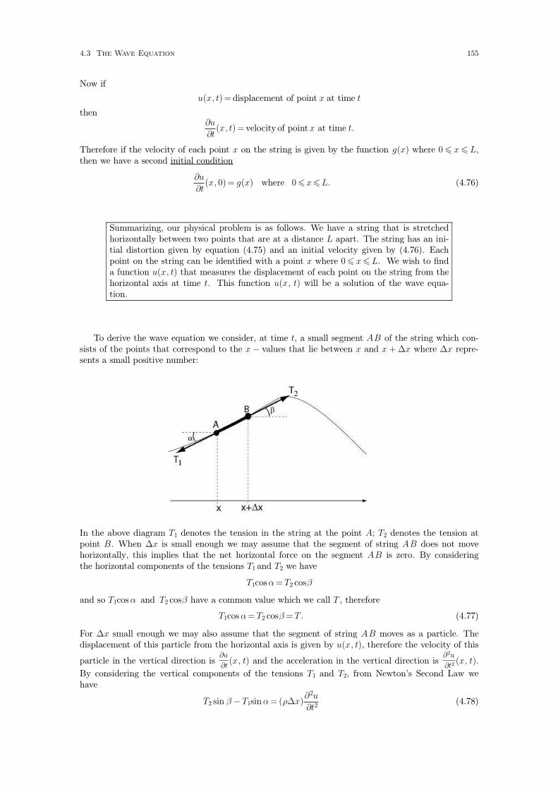
Now if
u(x, t)= displacement of point x at time t
then∂u
∂t(x, t) = velocity of pointx at time t.
Therefore if the velocity of each point x on the string is given by the function g(x) where 0 6 x 6 L,then we have a second initial condition
∂u
∂t(x, 0)= g(x) where 0 6x 6L. (4.76)
Summarizing, our physical problem is as follows. We have a string that is stretchedhorizontally between two points that are at a distance L apart. The string has an ini-tial distortion given by equation (4.75) and an initial velocity given by (4.76). Eachpoint on the string can be identified with a point x where 0 6 x 6 L. We wish to finda function u(x, t) that measures the displacement of each point on the string from thehorizontal axis at time t. This function u(x, t) will be a solution of the wave equa-tion.
To derive the wave equation we consider, at time t, a small segment AB of the string which con-sists of the points that correspond to the x − values that lie between x and x + ∆x where ∆x repre-sents a small positive number:
In the above diagram T1 denotes the tension in the string at the point A; T2 denotes the tension atpoint B. When ∆x is small enough we may assume that the segment of string AB does not movehorizontally, this implies that the net horizontal force on the segment AB is zero. By consideringthe horizontal components of the tensions T1 and T2 we have
T1cosα =T2 cosβ
and so T1cosα and T2 cosβ have a common value which we call T , therefore
T1cosα = T2 cosβ = T . (4.77)
For ∆x small enough we may also assume that the segment of string AB moves as a particle. Thedisplacement of this particle from the horizontal axis is given by u(x, t), therefore the velocity of this
particle in the vertical direction is∂u
∂t(x, t) and the acceleration in the vertical direction is
∂2u
∂t2(x, t).
By considering the vertical components of the tensions T1 and T2, from Newton’s Second Law wehave
T2 sin β −T1sinα = (ρ∆x)∂2u
∂t2(4.78)
4.3 The Wave Equation 155

where ρ is the mass per unit length of the string. Dividing equation (4.78) by the value T fromequation (4.77) we have
T2 sin β
T− T1sinα
T= (
ρ∆x
T)∂2u
∂t2
and using the expressions for T from equation (4.77) we have
T2 sin β
T2cosβ− T1sinα
T1cosα= (
ρ∆x
T)∂2u
∂t2
⇒ tan β − tanα =(ρ∆x
T)∂2u
∂t2.
(4.79)
In the following diagram the line segment BC is tangent to the curve u(x, t) at the point B (notethat we regard the t−variable as being fixed).
By the definition of slope we have
slope of tangent BC =CD
BD= tan β.
However, from the definition of the partial derivative
slope of tangent BC =∂u
∂x(x +∆x, t)
and therefore the slope of the tangent at B is
∂u
∂x(x +∆x, t)= tan β.
Similarly the slope of the tangent at A is∂u
∂x(x, t) = tanα
and from the equations of (4.79) we have
∂u
∂x(x +∆x, t)− ∂u
∂x(x, t)= (
ρ∆x
T)∂2u
∂t2.
Rearranging this equation gives
∂u
∂x(x +∆x, t)− ∂u
∂x(x, t)
∆x= (
ρ
T)∂2u
∂t2(4.80)
and we take the limit of (4.80) as ∆x→ 0 to get
lim∆x→0
(
∂u
∂x(x +∆x, t)− ∂u
∂x(x, t)
∆x
)
= (ρ
T)∂2u
∂t2. (4.81)
156 Partial Differential Equations
By definition of the partial derivative
lim∆x→0
(
∂u
∂x(x +∆x, t)− ∂u
∂x(x, t)
∆x
)
=∂
∂x
(
∂u
∂x(x, t)
)
=∂2u(x, t)
∂x2
and so from equation (4.81) we obtain
∂2u(x, t)
∂x2=(
ρ
T)∂2u
∂t2(4.82)
and as ρ and T are positive constants we may write equation (4.82) in the standard form of thewave equation
∂2u
∂t2= c2∂
2u
∂x2
where c is a constant.
4.3.2 Solution of the wave equation by seperation of variables
The solution of the wave equation by the method of seperation of variables is similar to the solutionof the heat equation by seperation of variables that was done in Section 4.2.2. In solving the waveequation we shall
− assume a solution of the form
u(x, t)= X(x)T (t)
− substitute this solution into the wave equation to obtain
T ′′(t)c2T (t)
=X ′′(x)
X(x)= k
− consider the cases of k = a2, 0, − a2 and use boundary conditions to determine which of thesecases of k lead to nonzero solutions of the wave equation
− use the Superposition Principle to write these non-zero solutions in expressions thatresemble4.5
u(x, t)=∑
n=1
∞ (
ancos
(
nπct
L
)
+ bnsin
(
nπct
L
))
sin(
nπx
L
)
− use initial conditions and the half-range cosine/sine formulae
an =2
L
∫
0
L
f(x)sinnπx
Ldx
nπcbn
L=
2
L
∫
0
L
g(x)sinnπx
Ldx
to determine the constants an and bn, where f(x) and g(x) describe the initial displacementand velocity.
4.5. solutions may not always take this form
4.3 The Wave Equation 157

We illustrate the solution of the wave equation by the following example.
Example 4.18. Solve the wave equation
∂2u
∂t2=
∂2u
∂x2(4.83)
subject to the boundary conditions
u(0, t) = 0u(π, t) = 0
and initial conditions
u(x, 0) = sinx− 1
2sin 2x
∂u
∂t(x, 0)=0
where 06 x6 π.
Answer: We use the method of seperation of variables and therefore assume that our solution u(x, t)takes the form
u(x, t)=X(x)T (t). (4.84)
Substituting the solution (4.84) into wave equation (4.83) gives
∂2
∂t2(X(x)T (t)) =
∂2
∂x2(X(x)T (t))
⇒ X(x)T ′′(t) =X ′′(x)T (t)
⇒ T ′′(t)T (t)
=X ′′(x)
X(x)(4.85)
and the only way for equation (4.85) to hold is ifT ′′(t)
T (t)and
X ′′(x)
X(x)are both constant functions and
are equal to the same constant k. So we have
T ′′(t)T (t)
=X ′′(x)
X(x)= k (4.86)
where the constant k can be zero, negative or positive, that is
k =0,− a2 or a2
where a� 0. We now use the boundary conditions
u(0, t)= 0u(L, t)= 0
where t> 0 (4.87)
to show that the only non-zero solutions of the wave equation (4.83) with the boundary conditions(4.87) occur when k =− a2.
k = 0
If k =0 then from equation (4.84) we obtain two ordinary differential equations
T ′′(t)= 0
X ′′(x) = 0.
Solving these gives
T (t)= A′t+ B ′
X(x)= C ′x+ D ′ (4.88)
where A′, B ′,C ′ and D ′ are constants.
158 Partial Differential Equations

Substituting equations (4.88) into equation (4.84) gives
u(x, t) = (C ′x+ D ′)(A′t+ B ′) (4.89)
From the first boundary condition of (4.87) we get
u(0, t)= D ′(A′t+ B ′)≡ 0
for all values of t > 0, which implies that
D ′=0.
The second boundary condition gives
u(π, t) =πC ′(A′t+B ′)≡ 0
for all values of t > 0, which implies that
C ′= 0.
As the boundary conditions imply that
C ′ =0D ′=0
we have that when k =0, the corresponding solution (4.89) is identically equal to zero.
k = a2
If k = a2 then from equation (4.84) we obtain two ordinary differential equations
T ′′(t)− a2T (t)= 0
X ′′(x)− a2X(x)= 0.
Solving these gives
T (t)= A′′cosh(at)+ B ′′sinh(at)
X(x)= C ′′cosh(ax)+D ′′sinh(ax)(4.90)
where A′′, B ′′,C ′′ and D ′′ are constants.
Substituting equations (4.90) into equation (4.84) gives
u(x, t)= (C ′′cosh(ax) +D ′′sinh(ax))(A′′cosh(at)+ B ′′sinh(at)) (4.91)
From the first boundary condition of (4.87) we get
u(0, t)= (C ′′(1) +D ′′(0))(A′′cosh(at)+B ′′sinh(at))≡ 0
for all values of t > 0, which implies that
C ′′= 0.
The second boundary condition gives
u(π, t) = (D ′′sinh(aπ))(A′′cosh(at) +B ′′sinh(at))≡ 0
for all values of t > 0, and as sinh(aπ)� 0 when a� 0, this implies that
D ′′=0.
As the boundary conditions imply that
C ′′ =0D ′′=0
we have that when k = a2, the corresponding solution (4.91) is identically equal to zero.
4.3 The Wave Equation 159
k =− a2
The last possibility of k = − a2 will lead to non-zero solutions. Subsituting k = − a2 into equation(4.86) gives
T ′(t)T (t)
=X ′′(x)
X(x)=− a2
from which we obtain the two ordinary differential equations
T ′′(t)+ a2T (t)= 0 (4.92)
X ′′(x)+ a2X(x) = 0 (4.93)
By using the D-operator method, the general solution of (4.92) is
T (t) =A cos(at)+ B sin(at)
and the general solution of (4.93) is
X(x)= C cos(ax) +D sin(ax).
So we have solutions of the wave equation of the form
u(x, t)= (A cos(at) +B sin(at))(C cos (ax) +D sin (ax)). (4.94)
From the first boundary condition we get
u(0, t)= (A cos(at)+B sin(at))(C(1) +D(0))≡ 0
⇒ C(A cos(at)+B sin(at))≡ 0
⇒ C =0
and therefore the solutions take the form
u(x, t) = (a′ cos(at) + b′ sin(at))sin (ax) (4.95)
where a′=AD and b′=BD.
Imposing the second boundary condition on equation (4.95) gives
u(π, t) = (a′ cos(at) + b′ sin(at))sin (aπ)≡ 0
⇒ sin(aπ) = 0
and so the second boundary condition forces
a= k where k =1, 2, 3,�(note we do not consider k = 0 as this leads to the zero solution; k =− 1,− 2,� do not give solutionsthat are linearly independent of those corresponding to k = 1, 2, � ). Substituting each of these dif-ferent values of a into equation (4.95) implies that
(a1cos(t)+ b1sin(t))sin(x) , (a2cos(2t) + b2sin(2t))sin(2x) , (a3cos(3t)+ b3sin(3t))sin(3x),�are each solutions of the wave equation (4.83). So from by the Superposition Principle II on page133 we have that
u(x, t)=∑
n=1
∞(ancos(nt)+ bnsin(nt))sin(nx) (4.96)
is a solution of the wave equation (4.83) which, by construction, satisfies the boundary conditions.
Finally, we use the given initial conditions
u(x, 0) = sinx− 1
2sin 2x
∂u
∂x(x, 0)= 0
where 06 x6 π.
160 Partial Differential Equations

to determine the coefficients an, bn of the solution (4.96). Setting t=0 in (4.96) gives
u(x, 0) =∑
n=1
∞(ancos(0)+ bnsin(0))sin(n x)= sinx− 1
2sin 2x when 06 x 6π
⇒∑
n=1
∞ansin(n x)= sinx− 1
2sin 2x when 06 x6 π (4.97)
The left side of equation (4.97) is a Fourier sine series that represents the function sin x − 1
2sin 2x on
the interval 0 6 x 6 π. Such a sine series is called the sine half-range expansion of the functionsin x − 1
2sin 2x on the interval 0 6 x 6 π and from Lemma 3.23 on page 128, the coefficients an of
the left side of (4.97) are given by
an =2
L
∫
0
L
f(x)sinnπx
Ldx where n =1, 2,�
⇒ an =2
π
∫
0
π(
sinx− 1
2sin 2x
)
sin (nx) dx where n =1, 2,�Now if n is an integer, then
∫
0
π
sin(nx)sin (nx) dx=
∫
0
π
sin2(nx) dx
=
∫
0
π 1− cos(2nx)
2dx
=π
2
and when n� m are both integers
∫
0
π
sin(nx)sin (mx) dx =
∫
0
π cos(m−n)x− cos(m + n)x
2dx
=0.Therefore we have
a1 =2
π
∫
0
π(
sinx− 1
2sin 2x
)
sinx dx
=2
π
∫
0
π
sinx sinx dx− 1
π
∫
0
π
sin 2x sinx dx
=2
π.π
2− 1
π.0
=1and similarly
a2 =2
π
∫
0
π(
sinx− 1
2sin 2x
)
sin 2x dx
=2
π
∫
0
π
sinx sin2x dx− 1
π
∫
0
π
sin 2x sin2x dx
=2
π.0− 1
π.π
2
=− 1
2.
For ak where k > 2 we have
ak =2
π
∫
0
π(
sinx− 1
2sin 2x
)
sin kx dx
=2
π
∫
0
π
sinx sin kx dx− 1
π
∫
0
π
sin 2x sin kx dx
=2
π.0− 1
π.0
= 0
4.3 The Wave Equation 161

and therefore we have determined the an
a1 =1 a2 =− 1
2and an =0 for all n > 2. (4.98)
Differentiating the solution (4.96) partially with respect to t gives
∂u
∂t(x, t)=
∑
n=1
∞(−nansin(nt)+nbncos(nt))sin(nx)
and from the second initial condition we have
∂u
∂t(x, 0)=
∑
n=1
∞(−nansin(0)+nbncos(0))sin(nx)≡ 0 when 06 x 6π
which implies∑
n=1
∞nbnsin(nx)≡ 0 (4.99)
The left side of equation (4.99) is a Fourier sine series that represents the function 0 on the interval0 6 x 6 π and from Lemma 3.23 on page 128, the coefficients nbn of the left side of (4.99) are givenby
nbn =2
L
∫
0
L
f(x)sinnπx
Ldx where n =1, 2,�
⇒ nbn =2
π
∫
0
π
(0)sin (nx) dx where n = 1, 2,�⇒nbn = 0
⇒ bn = 0 where n =1, 2,� (4.100)
Substituting the values of the coefficients an and bn given by (4.98) and (4.100) into (4.96) we obtainour solution
u(x, t)= cos(t)sin(x)− 1
2cos(2t)sin(2x)
of the wave equation (4.83) that satisfies the given boundary and initial conditions.
162 Partial Differential Equations

4.4 Laplace’s equation
Laplace’s equation is a partial differential equation that does not involve the time variable t. InCartesian coordinates, the form of Laplace’s equation depends on dimension:
Laplace′s equation in 1dimensiond2u
dx2=0
Laplace′s equation in 2dimensions∂2u
∂x2+
∂2u
∂y2=0
Laplace′s equation in 3dimensions∂2u
∂x2+
∂2u
∂y2+
∂2u
∂y2= 0
Laplace’s equation arises when one considers solutions of physical problems that are independent oftime. Solutions that are independent of time are called steady state solutions.
Example 4.19. In Example 4.17 we showed on page 150 that
us(x, t)= 10x
is a solution of the heat equation
∂u
∂t= c2∂
2u
∂x2
subject to the nonhomogeneous boundary conditions
u(0, t) = 0u(10, t)= 100
where t> 0
Notice that the solution us does not involve the t variable, so us is an example of a steady-state solu-tion. As us is a solution of this heat equation we clearly have
∂us
∂t= c2∂
2us
∂x2. (4.101)
Furthermore as us is independent of the time variable t, when we differentiate partially with respectto t we have
∂us
∂t=0 (4.102)
and substituting (4.102) into (4.101) we have that, after dividing by c2, that
∂2us
∂x2= 0
and as us is a function of x only we have that
d2us
dx2=0
which is Laplace’s equation in one dimension. So we see that us is an example of a steady-state solu-tion of a one-dimensional heat equation being a solution of Laplace’s equation in one-dimension.
To be precise, us is a solution of the Laplace’s equation together with specified boundary conditions:
4.4 Laplace’s equation 163

d2u
dx2= 0
subject to the boundary conditions
u(0)= 0u(10) = 100
Finally, recall that the limit of the solution of the heat equation in Example 4.17
limt→∞
u(x, t)= limt→∞
(
10x−∑
k=0
∞800
(2k +1)3π3e−c2
(
(2k+1)π
10
)2tsin
(
(2k +1)πx
10
)
)
= 10x= us(x, t)
So we see that the steady-state solution us of the the heat equation in Example 4.17 gives the tem-perature distribution that the metal bar eventually stabilizes to. As us is a solution of a Laplace’sequation, we have that the limiting temperature distribution of the solution of a heat equation cansometimes be obtained as a solution of a corresponding Laplace’s equation with the appropriateboundary conditions.
We see an example of this in the following
Example 4.20. From Example 4.14 we saw the solution of the following heat equation problem
Let u(x, t) denote the temperature of a thin metal bar of length 1 that is insulatedalong the sides. Let the temperature along the length of the bar at time t = 0 begiven by
u(x, 0)=4x(1−x) where 06 x6 1.
The ends of the bar are kept at a constant temperature of 0, that is
u(0, t)= 0u(1, t)= 0
where t> 0.
is given by
u(x, t)=∑
k=0
∞32
(2k +1)3π3e−c2((2k+1)π)2tsin((2k +1)πx)
and this temperature function eventually stablilizes to
limt→∞
u(x, t)= 0 (4.103)
as we would expect because all the initial heat in the bar flows out of the ends of the bar which areat zero temperature. Notice that this limiting temperature distribution of zero (4.103) is identical tothe solution of a corresponding one-dimensional Laplace’s equation with the same boundary condi-tions as the heat equation
d2u
dx2= 0
subject to the boundary conditions
u(0)= 0u(1)= 0
164 Partial Differential Equations
because the solution of the above Laplace’s equation is easily shown to be zero:
d2u
dx2=0
⇒ u(x)=Ax+ Band the boundary conditions
u(0)= 0u(1)= 0
imply that
A =B = 0
hence
u= 0.
which is the limiting temperature distribution of (4.103).
The previous two examples provide evidence that Laplace’s equation in one dimension can be inter-preted as a steady-state heat flow problem in one dimension, that is, a problem of finding asteady-state solution of a one dimensional heat equation that satisfies some given boundary condi-tions.
In this section we shall be interested in solving the two dimensional Laplace’s equation over a rect-angular domain. The following lemma implies that Laplace’s equation in two dimensions can also beinterpreted as a steady-state heat flow problem in two dimensions, that is, a problem of finding asteady-state solution of a two dimensional heat equation that satisfies certain conditions on theboundary of the domain.
Lemma 4.21. Let us be a steady-state solution of the two dimensional heat equation
∂u
∂t= c2
(
∂2u
∂x2+
∂2u
∂y2
)
. (4.104)
Then us is a solution of Laplace’s equation in two dimensions
∂2u
∂x2+
∂2u
∂y2=0.
Proof. As us is a solution of this heat equation we clearly have
∂us
∂t= c2
(
∂2us
∂x2+
∂2us
∂y2
)
(4.105)
As us is steady-state, it is independent of the time variable t and therefore
∂us
∂t= 0 (4.106)
and by substituting (4.106) into (4.105) and dividing by c2 we have that
∂2us
∂x2+
∂2us
∂y2= 0
and therefore us is a solution of Laplace’s equation in two dimensions.�
4.4 Laplace’s equation 165

4.4.1 Solving Laplace’s equation by seperation of variables
We illustrate the solution of Laplace’s equation over a rectangular domain with prescribed boundaryconditions by the following example.
Example 4.22. By solving Laplace’s equation
∂2u
∂x2+
∂2u
∂y2= 0 (4.107)
in the square domain
{(x, y)| 06 x 6 1 and 06 y 6 1},
find the steady-state temperature u(x, y) of a thin square metal plate of length 1 which has each ofits four sides at temperatures that are given by the following boundary conditions
u(0, y)= 0u(1, y)= 0u(x, 0)= 0u(x, 1) =x(1−x)
where 06 x6 1 and 0 6 y 6 1. (4.108)
Answer: The following diagram illustrates the boundary conditions around the square plate:
We solve this Laplace’s equation by using seperation of variables and therefore assume that our solu-tion u(x, y) takes the form
u(x, y)=X(x)Y (y). (4.109)
Substituting the solution (4.109) into Laplace’s equation (4.107) gives
∂2
∂x2(X(x)Y (y))+
∂2
∂y2(X(x)Y (y))= 0
⇒ X ′′(x)Y (y)+ X(x)Y ′′(y)= 0
⇒ X ′′(x)
X(x)=− Y ′′(y)
Y (y)(4.110)
166 Partial Differential Equations

and the only way for equation (4.85) to hold is ifX ′′(x)
X(x)and − Y ′′(y)
Y (y)are both constant functions
and are equal to the same constant k. So we have
X ′′(x)
X(x)=− Y ′′(y)
Y (y)= k (4.111)
where the constant k can be zero, negative or positive, that is
k =0,− a2 or a2
where a � 0. As with the heat and wave equations, we use the boundary conditions (4.108) to deter-mine which of the k =0,− a2 or a2 will give non-zero solutions.
k = 0
If k =0 then from equation (4.111) we obtain two ordinary differential equations
X ′′(x)= 0
Y ′′(y) = 0.
Solving these givesX(x)= A′x+ B ′
Y (y)=C ′y + D ′ (4.112)
where A′, B ′,C ′ and D ′ are constants.
Substituting equations (4.112) into equation (4.109) gives
u(x, y)= (A′x+ B ′)(C ′y +D ′)
and it is easy to check that the boundary conditions
u(0, y)= 0u(1, y)= 0
imply that A′=B ′= 0 and hence the only solution u(x, y) corresponding to k = 0 is the zero solution
u(x, y) = 0.
k = a2
If k = a2 then from equation (4.111) we obtain two ordinary differential equations
X ′′(x)− a2X(x)= 0
Y ′′(y)− a2Y (y)= 0.
Solving these givesX(x) =A′′cosh(ax)+B ′′sinh(ax)
Y (y)=C ′′cosh(ay)+D ′′sinh(ay)(4.113)
where A′′, B ′′,C ′′ and D ′′ are constants.
Substituting equations (4.113) into equation (4.111) gives
u(x, y)= (A′′cosh(ax)+B ′′sinh(ax))(C ′′cosh(ay)+D ′′sinh(ay))
and again it is easy to check that the boundary conditions
u(0, y)= 0u(1, y)= 0
4.4 Laplace’s equation 167

imply that A′′ = B ′′ = 0 and hence the only solution u(x, y) corresponding to k = a2 is the zero solu-tion
u(x, y) = 0.
k =− a2
The last possibility of k = − a2 will lead to non-zero solutions. Subsituting k = − a2 into equation(4.111) gives
X ′′(x)
X(x)=− Y ′′(y)
Y (y)=− a2
from which we obtain the two ordinary differential equations
X ′′(x)+ a2X(x) = 0
Y ′′(y)− a2Y (y)= 0
Solving these givesX(x)= A cos(ax) +B sin(ax)Y (y)= C cosh(ay)+ D sinh (ay)
(4.114)
where A, B, C and D are constant. Substituting (4.114) into (4.109) gives
u(x, y) = (A cos(ax)+B sin(ax))(C cosh(ay)+D sinh (ay)).
From the first boundary condition
u(0, y)= 0
of (4.108) we have
u(0, y)= (A cos(0)+ B sin(0))(C cosh(ay) +D sinh (ay))≡ 0
⇒ A(C cosh(ay)+D sinh (ay))≡ 0
⇒ A = 0
and therefore our solution u(x, y) takes the form
u(x, y) = sin(ax)(a′cosh(ay)+ b′sinh(ay)) (4.115)
where a′=BC and b′= BD.
Imposing the second boundary condition
u(1, y)= 0
on the solution (4.115) gives
u(1, y) = sin(a)(a′cosh(ay)+ b′sinh(ay))≡ 0
⇒ sin(a)= 0
and so the second boundary condition forces
a= kπ where k = 1, 2, 3,�Substituting each of these different values of a into (4.115) implies that
sin(πx)(a1cosh(πy)+ b1sinh(πy))
sin(2πx)(a2cosh(2πy) + b2sinh(2πy))
sin(3πx)(a3cosh(3πy) + b3sinh(3πy))are each solutions of Laplace’s equation. So from the Superposition Principle we have that
u(x, y) =∑
n=1
∞sin(nπx)(ancosh(nπy) + bnsinh(nπy)) (4.116)
is a general form of the solution of Laplace’s equation which, by construction, satisfies the first twoboundary conditions of (4.108).
168 Partial Differential Equations

Finally, we use the other two boundary conditions
u(x, 0)= 0u(x, 1) =x(1−x)
when 06 x6 1
to determine the coefficients an, bn of the solution (4.116). From
u(x, 0)=0
we have
u(x, 0) =∑
n=1
∞sin(nπx)(ancosh(0)+ bnsinh(0))= 0
⇒∑
n=1
∞sin(nπx)(an(1)+ bn(0))= 0
⇒∑
n=1
∞ansin(nπx)= 0 when 06 x 6 1. (4.117)
The left side of equation (4.117) is a Fourier sine series that represents the function 0 on the interval0 6 x 6 1 and from Lemma 3.23 on page 128, the coefficients an on the left side of (4.117) are givenby
an =2
L
∫
0
L
f(x)sinnπx
Ldx where n = 1, 2,�
⇒ an =2
1
∫
0
1
(0)sinnπx dx where n =1, 2,�⇒ an =0 where n =1, 2,�
and so we have that our solution (4.116) of Laplace’s equation simplifies to
u(x, y)=∑
n=1
∞bnsin(nπx)sinh(nπy). (4.118)
From the fourth boundary condition
u(x, 1) =x(1− x)
we have
u(x, 1)=∑
n=1
∞bnsin(nπx)sinh(nπ) =x(1− x) when 06 x6 1
⇒∑
n=1
∞(bnsinh (nπ))sin(nπx) =x(1−x) when 06 x6 1. (4.119)
The left side of equation (4.119) is a Fourier sine series with coefficients
bnsinh(nπ)
that represents the function x(1 − x) on the interval 0 6 x 6 1 and from Lemma 3.23 on page 128,the coefficients bnsinh(nπ) on the left side of (4.119) are given by
bnsinh(nπ) =2
1
∫
0
1
x(1− x)sinnπx
1dx where n =1, 2,�
Integrating
2
∫
0
1
x(1− x)sin (nπx)dx
by parts withv = x(1− x) du = sin(nπx)dx
dv = (1− 2x) dx u=− cos (nπx)
nπgives
bnsinh(nπ)= 2
[
− x(1− x)cos (nπx)
nπ
]
0
1
+ 2
∫
0
1 (1− 2x)cos (nπx)
nπdx
= 0 +2
∫
0
1 (1− 2x)cos (nπx)
nπdx
4.4 Laplace’s equation 169

Integrating by parts again with
v = (1− 2x) du =cos (nπx)
nπdx
dv =− 2 dx u =sin (nπx)
n2π2gives
bnsinh(nπ)= 2
[
(1− 2x)sin (nπx)
n2π2
]
0
1
+2
∫
0
1 2sin (nπx)
n2π2dx
=0 + 2
[
− 2cos (nπx)
n3π3
]
0
1
=2
(
− 2(− 1)n
n3π3+
2
n3π3
)
=
0 when n is even
8
n3π3 when n is odd
and therefore
bn =
0 when n is even
8
n3π3sinh(nπ)when n is odd
Substituting these values for bn into (4.118) and writing the odd values of n as 2k + 1 gives our solu-tion for u(x, y)
u(x, y)=∑
k=0
∞8
(2k +1)3π3sinh((2k +1)π)sin((2k + 1)πx)sinh((2k +1)πy) (4.120)
which gives the steady-state temperature distribution of the square plate with the given boundaryconditions.
The following contour plot, drawn with the computer program Maple, shows a plot of the solu-tion (4.120) that represents a temperature distribution of the square plate (for example, all points onthe curve labelled u = .04 have temperature equal to .04). Note that the maximum temperature of.25 on the square plate is achieved at the point
(x, y)= (.5, 1)
which lies on the top edge of the plate.
Figure 4.1. Contour plot showing steady-state solution to Example 4.22
170 Partial Differential Equations

4.5 Laplace’s equation in polar coordinates
In the last section we used Laplace’s equation
∂2u
∂x2+
∂2u
∂y2= 0 (4.121)
to solve a steady-state heat flow problem in a square plate. If we wish to solve similar problems incircular plates, it is sometimes easier to work with polar coordinates (r, θ) than with Cartesiancoordinates (x, y).
Recall that a point may be located in the plane by its Cartesian coordinates (x, y). The locationof this same point may also be given by the polar coordinates (r, θ)
Figure 4.2.
where r is the distance of the point (x, y) from the origin and θ is the angle that the line connectingthe point (x, y) with the origin makes with the x − axis. By considering the above right-angled tri-angle, clearly we have
x= r cos θ (4.122)
y = r sin θ. (4.123)
Let
u(x, y) (4.124)
be a solution of the two-dimensional Laplace’s equation (4.121). Then if we replace x in the solutionu(x, y) by equation (4.122) and replace y by equation (4.123) we obtain a function
u(r cos θ, r sin θ) (4.125)
in the variables r and θ. We will prove in Lemma 4.27 that the function (4.125) is a solution of thepartial differential equation
∂2u
∂r2+
1
r
∂u
∂r+
1
r2
∂2u
∂θ2=0 (4.126)
and the equation (4.126) is called Laplace’s equation in polar coordinates.
The opposite is also true (we will not prove this). If w(r, θ) is a solution of Laplace’s equation inpolar coordinates, then by using the substitutions
r =(x2 + y2)1
2 (4.127)
θ = tan−1(
y
x
)
. (4.128)
we can ‘convert’ w(r, θ) into a function of the variables x and y
w((x2 + y2)1
2, tan−1(
y
x
)
)
4.5 Laplace’s equation in polar coordinates 171

and this function will be a solution of Laplace’s equation (4.121) in Cartesian coordinates.
Example 4.23. By differentiating partially, it is easy to check that the function u(x, y) = x is asolution of Laplace’s equation
∂2u
∂x2+
∂2u
∂y2=0.
Expressing this solution u in polar coordinates gives
u(r, θ) = r cos θ
and this function of (r, θ) satisfies Laplace’s equation (4.121) in polar coordinates
∂2u
∂r2+
1
r
∂u
∂r+
1
r2
∂2u
∂θ2
=∂2
∂r2(r cos θ)+
1
r
∂
∂r(r cos θ)+
1
r2
∂2
∂θ2(r cos θ)
= 0 +1
r(cos θ)+
1
r2(− r cos θ)
= 0
Recall the following basic result for derivatives of functions of one variable.
Lemma 4.24. (Chain Rule) If y = f(u) and u = g(x) are both differentiable functions then
y = f(g(x))
is a differentiable function of x anddy
dx=
dy
du· du
dx
Example 4.25. Let y =u10 and u =x2 +x. Then from Lemma 4.24
y = (x2 + x)10
is a differentiable function of x anddy
dx= 10u9 · (2x +1)
= 10(x2 +x)9(2x+ 1).
For functions of two variables, there is also a version of the Chain Rule which we will state in theform that we shall need.
Lemma 4.26. Suppose that u(r, θ) is a differentiable function of r and θ. Let
r = g(x, y)θ = h(x, y)
and suppose that the partial derivatives∂r
∂x,∂r
∂y,∂θ
∂xand
∂θ
∂yexist. Then
u(g(x, y), h(x, y))
is a differentiable function of x and y and
∂u
∂x=
∂u
∂r· ∂r
∂x+
∂u
∂θ· ∂θ
∂x
∂u
∂y=
∂u
∂r· ∂r
∂y+
∂u
∂θ· ∂θ
∂y
172 Partial Differential Equations

We now show that a solution u(x, y) of Laplace’s equation in Cartesian coordinates corresponds to asolution u(r cos θ, r sin θ) of Laplace’s equation in polar coordinates.
Lemma 4.27. Let u(x, y) be a solution of Laplace’s equation
∂2u
∂x2+
∂2u
∂y2=0.
Then the function u(r cos θ, r sin θ) 4.6 is a solution of
∂2u
∂r2+
1
r
∂u
∂r+
1
r2
∂2u
∂θ2=0
which is Laplace’s equation in polar coordinates.
Proof. Let u(x, y) be a solution of Laplace’s equation. If we replace x, y in u(x, y) by
x= r cos θ
y = r sin θwe obtain the function
u(r cos θ, r sin θ). (4.129)
We shall apply Lemma 4.26 to the function (4.129). The corresponding functions r, θ of Lemma 4.26shall be
r =(x2 + y2)1
2 (4.130)
θ = tan−1(
y
x
)
(4.131)
From Figure 4.2 we have
cos θ =adjacent
hypotenuse=
x
(x2 + y2)1
2
sin θ =opposite
hypotenuse=
y
(x2 + y2)1
2
Substituting (4.130) and (4.131) into (4.129) gives
u(r cos θ, r sin θ)
=u
(
(x2 + y2)1
2x
(x2 + y2)1
2
, (x2 + y2)1
2y
(x2 + y2)1
2
)
(4.132)
and notice that the function of x and y given in (4.132) is nothing but the solution u(x, y) ofLaplace’s equation
u
(
(x2 + y2)1
2x
(x2 + y2)1
2
, (x2 + y2)1
2y
(x2 + y2)1
2
)
=u(x, y).
Applying Lemma 4.26 to (4.132) gives
∂u
∂x=
∂u
∂r· ∂r
∂x+
∂u
∂θ· ∂θ
∂x
=∂u
∂r· x
(x2 + y2)1
2
+∂u
∂θ·(
− y
(x2 + y2)
)
⇒ ∂u
∂x=
∂u
∂r· x
r+
∂u
∂θ·(
− y
r2
)
(4.133)
where r is as given in (4.130).
4.6. The functions u(x, y) and u(r cos θ, r sin θ) are the same function expressed in different coordinates.
4.5 Laplace’s equation in polar coordinates 173

Also∂u
∂y=
∂u
∂r· ∂r
∂y+
∂u
∂θ· ∂θ
∂y
=∂u
∂r· y
(x2 + y2)1
2
+∂u
∂θ·(
x
(x2 + y2)
)
⇒ ∂u
∂y=
∂u
∂r· y
r+
∂u
∂θ·(
x
r2
)
(4.134)
Notice that equations (4.133) and (4.134) express the partial derivatives of the solu-tion u(x, y) in terms of the partial derivatives of u(r cos θ, r sin θ). Similarly, we wantto express the second partial derivatives
∂2u
∂x2,
∂2u
∂y2
of the solution u(x, y) in terms of the second partial derivatives of u(r cos θ, r sin θ).Then the equation
∂2u
∂x2+
∂2u
∂y2= 0
will give a relationship among the second partial derivatives of u(r cos θ, r sin θ), thisrelationship will be exactly Laplace’s equation in polar coordinates
∂2u
∂r2+
1
r
∂u
∂r+
1
r2
∂2u
∂θ2=0
and the fact that the partial derivatives of u(r cos θ, r sin θ) satisfy this relationshipmeans that u(r cos θ, r sin θ) is a solution of Laplace’s equation in polar coordinates.
So we differentiate (4.133) with respect to x, by first applying the product rule and then chain rulein the form of Lemma 4.26
∂2u
∂x2=
∂
∂x
(
∂u
∂r
)
· x
r+
∂u
∂r· ∂
∂x
(
x
r
)
+∂
∂x
(
∂u
∂θ
)
·(
− y
r2
)
+∂u
∂θ· ∂
∂x
(
− y
r2
)
=∂
∂x
(
∂u
∂r
)
· x
r+
∂u
∂r· y2
r3+
∂
∂x
(
∂u
∂θ
)
·(
− y
r2
)
+∂u
∂θ· 2xy
r4
=
(
∂2u
∂r2· x
r+
∂2u
∂θ∂r·(
− y
r2
))
· x
r+
∂u
∂r· y2
r3+
(
∂2u
∂r∂θ· x
r+
∂2u
∂θ2·(
− y
r2
))
·(
− y
r2
)
+∂u
∂θ· 2xy
r4
⇒ ∂2u
∂x2=
∂2u
∂r2· x2
r2− ∂2u
∂θ∂r· 2xy
r3+
∂2u
∂θ2· y2
r4+
∂u
∂r· y2
r3+
∂u
∂θ· 2xy
r4(4.135)
Similarly, by differentiating (4.134) with respect to y gives
∂2u
∂y2=
∂2u
∂r2· y2
r2+
∂2u
∂θ∂r· 2xy
r3+
∂2u
∂θ2· x2
r4+
∂u
∂r· x2
r3− ∂u
∂θ· 2xy
r4(4.136)
by adding (4.135) and (4.136) we have
∂2u
∂x2+
∂2u
∂y2=
(
x2 + y2
r2
)
∂2u
∂r2+
(
x2 + y2
r3
)
∂u
∂r+
(
x2 + y2
r4
)
∂2u
∂θ2. (4.137)
The function u(x, y) on the left of (4.137) which is a solution of Laplace’s equation by hypothesis
∂2u
∂x2+
∂2u
∂y2= 0
and substituting this in (4.137) and using the equation
r2 = x2 + y2
174 Partial Differential Equations

gives the following relationship between the partial derivatives of u(r cos θ, r sin θ)
∂2u
∂r2+
1
r
∂u
∂r+
1
r2
∂2u
∂θ2=0
which implies that u(r cos θ, r sin θ) is a solution of Laplace’s equation in polar coordinates. �
We illustrate Laplace’s equation in polar coordinates by the following example.
Example. By solving Laplace’s equation in polar coordinates
∂2u
∂r2+
1
r
∂u
∂r+
1
r2
∂2u
∂θ2= 0 (4.138)
in the circular domain
{(r, θ)|r 6 1}find the steady-state temperature of a thin metal disc of radius 1 which has boundary temperaturespecified by
u(1, θ)= sin3θ 06 θ 6 2π. (4.139)
Answer: The following diagram illustrates the boundary condition around the metal disc
We use the method of seperation of variables and therefore assume that our solution u(r, θ) takesthe form
u(r, θ)= R(r)Θ(θ). (4.140)
Substituting the solution (4.84) into Laplace’s equation in polar coordinates (4.138) gives
∂2
∂r2(R(r)Θ(θ))+
1
r
∂
∂r(R(r)Θ(θ))+
1
r2
∂2
∂θ2(R(r)Θ(θ))= 0
⇒ R ′′(r)Θ(θ)+1
rR ′(r)Θ(θ)+
1
r2R(r)Θ′′(θ) = 0
⇒ (r2 R′′(r) + rR ′(r))Θ(θ)=−R(r)Θ′′(θ)
⇒ r2 R′′(r)+ rR′(r)R(r)
=− Θ′′(θ)Θ(θ)
(4.141)
and the only way for equation (4.85) to hold is ifr2 R ′′(r) + rR ′(r)
R(r)and − Θ ′′(θ)
Θ(θ)are both constant
functions and are equal to the same constant k. So we have
r2 R ′′(r)+ rR′(r)R(r)
=− Θ′′(θ)Θ(θ)
= k (4.142)
4.5 Laplace’s equation in polar coordinates 175

where the constant k can be zero, negative or positive, that is
k =0,− a2 or a2
where a> 0.
Now notice that
(r, θ) , (r, θ +2π), (r, θ +4π),�specifiy exactly the same point in polar coordinates. It follows that the function u(r, θ) should havethe following property
u(r, θ) =u(r, θ +2kπ)
where k is an integer. Therefore from equation (4.140) we have
R(r)Θ(θ) =R(r)Θ(θ +2kπ)
⇒ Θ(θ)= Θ(θ +2kπ)
that is, the function Θ(θ) must be periodic with period 2π. This fact implies that the constant k of
equation (4.142) cannot be negative, that is k� − a2, because
− Θ′′(θ)Θ(θ)
=− a2
⇒ Θ′′(θ)− a2 Θ(θ)= 0
⇒ Θ(θ) =Ae−aθ + Beaθ
and this function is only periodic if A = B =0.
We now consider the other two possibilities k =0 and k = a2 .
k = 0
If k =0 then from equation (4.142) we obtain two ordinary differential equations
r2 R′′(r) + rR ′(r)= 0
Θ′′(θ) = 0
Solving these 4.7 gives
R(r)=A′ +B ′ ln r (4.143)
Θ(θ)=C ′ +D ′θ (4.144)
where A′, B ′,C ′ and D ′ are constants. Now from above, the function Θ(θ) must be periodic, andtherefore D ′= 0, hence
Θ(θ)=C ′ (4.145)
(note that a constant function is periodic).
Substituting equations (4.143) and (4.145) into equation (4.140) gives
u(r, θ)= a+ b ln r (4.146)
where a=A′C ′ and b=B ′C ′.
Now for this steady-state heat problem, we expect that the temperature at r = 0 (that is at thecenter of the disc) to have some finite value as the condition
u(1, θ)= sin3θ 06 θ 6 2π
4.7. We can solve r2 R′′(r) + rR ′(r)= 0 by using the substitution w = R′(r) and then seperating variables.
176 Partial Differential Equations
imposes finite temperature on the boundary. Note however, that if b� 0 in the solution (4.146) then
limr→0+
a+ b ln r =±∞depending on the sign of b because
limr→0+
ln r =−∞.
Because we expect finite temperature at r =0, we have that b=0 in (4.146) and therefore
u(r, θ)= a
is the only possible solution of Laplace’s equation in polar coordinates when the constant k = 0 inequation (4.142). Because we shall eventually use Fourier series, we write this solution as
u(r, θ)=a0
2. (4.147)
k = a2
If k = a2 then from equation (4.142) we obtain two ordinary differential equations
r2 R ′′(r)+ rR ′(r)− a2R(r) = 0 (4.148)
Θ ′′(θ)+ a2Θ(θ)= 0 (4.149)
The solution of (4.149) is
Θ(θ)= A′′cos(aθ) +B ′′sin(aθ).
and because Θ(θ) must be periodic with period 2π, it follows that
a= n= 1, 2, 3,�Substituting a=n into (4.148) gives
r2 R ′′(r)+ rR ′(r)−n2R(r)= 0
and this differential equation is called Euler’s equation. By substitution it is easy to check thatthe general solution of Euler’s equation is
R(r)=C ′′rn +D ′′r−n
and so, by substituting in (4.140), for each value of n =1, 2, 3,� we have a corresponding solution
un(r, θ)= (Cn′′rn +Dn
′′r−n)(An′′cos(nθ)+ Bn
′′sin(nθ)) (4.150)
As discussed above, we expect that the temperature at r = 0 (that is at the center of the disc) tohave some finite value. Note however, that
limr→0+
r−n =∞,
this implies that for each n = 1, 2, 3,� we have that the constant
Dn′′=0
and so for each value of n =1, 2, 3,� we have the corresponding solution
un(r, θ)= rn(ancos(nθ) + bnsin(nθ))
where an =Cn′′An
′′ and bn =Cn′′Bn
′′.
So we see that for k = 0 and k =1, 2,� the functions
a0
2, r(a1cos(θ)+ b1sin(θ)), r2(a2cos(2θ) + b2sin(2θ)), �
4.5 Laplace’s equation in polar coordinates 177

are each solutions of this particular Laplace’s equation in polar coordinates. So from the Superposi-tion Principle we have that
u(r, θ) =a0
2+∑
n=1
∞rn(ancos(nθ) + bnsin(nθ)) (4.151)
is the form of the solution of our Laplace’s equation in polar coordinates. We determine the con-stants an and bn of (4.151) from the given boundary condition
u(1, θ)= sin3θ when 0 6 θ 6 2π.
Substituting r = 1 into (4.151) implies that
a0
2+∑
n=1
∞(ancos(nθ) + bnsin(nθ))= sin3θ when 06 θ 6 2π. (4.152)
The left side of (4.152) is nothing but the Fourier series of sin3θ for the interval 0 6 θ 6 2π. There-fore, from the Euler’s formulae for a Fourier series we have
an =1
π
∫
−π
π
sin3θcos(nθ) dθ where n =0, 1, 2, 3,�bn =
1
π
∫
−π
π
sin3θ sin(nθ)dθ where n = 1, 2, 3,�Notice that the function
sin3θ
is an odd function, therefore we have that
an = 0 for each n =0, 1, 2, 3,�To determine the bn we recall the triple angle formula
sin 3θ =3sinθ − 4sin3θ
⇒ sin3θ =3
4sinθ − 1
4sin 3θ
Also recall that if n is an integer, then
∫
−π
π
sin(nθ)sin (nθ) dθ =
∫
−π
π
sin2(nθ) dθ
=
∫
−π
π 1− cos(2nθ)
2dθ
=π
and when n� m are both integers
∫
−π
π
sin(nθ)sin (mθ) dθ =
∫
−π
π cos(m−n)θ − cos(m +n)θ
2dθ
=0.
(4.153)
Therefore we have
b1 =1
π
∫
−π
π
sin3θ sin θ dθ
=1
π
∫
−π
π
(3
4sinθ − 1
4sin 3θ) sin θ dθ
=1
π
∫
−π
π 3
4sinθ sin θ dθ − 1
π
∫
−π
π 1
4sin 3θ sin θ dθ
=1
π.3
4π − 1
π.0
=3
4
178 Partial Differential Equations

and similarly
b3 =1
π
∫
−π
π
sin3θ sin 3θ dθ
=1
π
∫
−π
π
(3
4sinθ − 1
4sin 3θ) sin 3θ dθ
=1
π
∫
−π
π 3
4sinθ sin 3θ dθ − 1
π
∫
−π
π 1
4sin 3θ sin3θ dθ
=1
π.0− 1
π.1
4π
=− 1
4.
For any positive integer n� 1, 3 we have
bn =1
π
∫
−π
π
sin3θ sinnθ dθ
=1
π
∫
−π
π
(3
4sinθ − 1
4sin 3θ) sinnθ dθ
=1
π
∫
−π
π 3
4sinθ sinnθ dθ − 1
π
∫
−π
π 1
4sin 3θ sinnθ dθ
=1
π.0− 1
π.0 (from the identity (4.153))
= 0and substituting
an = 0 for each n =0, 1, 2, 3,�bn =
3
4n = 1
− 1
4n = 3
0 otherwise
into (4.151) we obtain the solution of Laplace’s equation in polar coordinates
u(r, θ) =3
4r sinθ − 1
4r3 sin 3θ
that satisfies the given boundary condition (4.139).
4.5 Laplace’s equation in polar coordinates 179

180 Partial Differential Equations